Astrokit—an Efficient Program for High-Precision Differential CCD Photometry and Search for Variable Stars

Having a need to perform differential photometry for tens of thousands stars in a several square degrees field, we developed Astrokit program. The software corrects the star brightness variations caused by variations of atmospheric transparency: to this end, the program selects for each star an individual ensemble of reference stars having similar magnitudes and positions in the frame. With ten or more reference stars in the ensemble, the differences between their spectral types and the spectral type of the object studied become unimportant. Astrokit searches for variable stars using Robust Median Statistics criterion, which allows candidate variables to be selected more efficiently than by analyzing the standard deviation of star magnitudes. The software allows very precise automatic analysis of long inhomogeneous sets of photometric observations of a large number of objects to be performed, making it possible to find “hot Jupiter” type exoplanet transits and low-amplitude variables. We describe the algorithm of the program and the results of its application to reduce the data of the photometric sky survey in Cygnus as well as observations of the open cluster NGC 188 and the transit of the exoplanet WASP-11 b / HAT-P-10 b, performed with the MASTER-II-URAL telescope of the Kourovka Astronomical Observatory of the Ural Federal University.

1 Introduction

We developed Astrokit C++ console application for post-processing of the results of CCD photometry within the framework of a program for the search for new variable stars and exoplanet transits in the Kourovka Astronomical Observatory of the Ural Federal University. The application is based on an upgraded algorithm of differential photometry using ensembles of comparison stars as described in Everett & Howell (2001).

In this paper we do not consider the sources of errors that influence the precision of CCD photometry. For a detailed discussion and analysis of this problem and the use of other methods of CCD photometry see Howell et al. (1988); Gilliland & Brown (1988, 1992); Newberry (1991); Young et al. (1991); Honeycutt (1992); Gilliland et al. (1993); Merline & Howell (1995); Howell & Everett (2001); Everett et al. (2001). We only recall that the idea of differential photometry consists in determining the difference between the magnitude of the source studied and that or those of one or several reference stars, thereby reducing the influence of time-variable atmospheric effects. In the ideal case the reference star should have similar brightness, color index, and must be located close to the star studied.

The close location of the reference stars to the star studied is especially important in the case of the reduction of wide-field images. This is because otherwise local variations of atmospheric transparency would have different effect on the reference sources and on the object studied, thereby inevitably degrading the resulting photometric precision.

After performing differential photometry Astrokit searches for variable stars. Below we describe the algorithm of the program, its implementation, and some of the results obtained.

2 Method

Before starting post-processing of the photometric data, photometry proper has to be performed. It makes no difference what software was used to extract fluxes from the CCD frame, the only important thing is to obtain the corresponding magnitudes and their theoretical errors in accordance with the main CCD equation (Howell (1993)).

For the studies carried out at the Astronomical Observatory of Ural Federal University, a dedicated technique of photometric reduction was developed within the framework of IRAF package (Tody (1986)).Before applying IRAF the console version ofAstrometry.net application (Lang et al. (2010)) is used to set the correct World Coordinate System parameters in the FITS header of each frame. IRAF package is then used to perform photometric reduction of each frame: subtraction of the dark frame and dividing by the flat-field frame. The PHOT/APPHOT task is then used to perform aperture photometry in each frame with individual aperture and sky background values for each frame. A catalog of objects containing the equatorial coordinates and running numbers of stars is used to this end. The aperture radius used in each particular frame is set equal to $0.8\,{\rm FWHM}$, where $\rm FWHM$ is the mean full width at half maximum value of the stellar PSF in the frame. The resulting data are then transferred to Astrokit, whose general structure is shown in Fig. 1.

Input data for the program are contained in the file created by PDUMP command of IRAF package and include:

• identification number of the star (id),

• number of counts (analog-to-digital units) from the star inside the aperture together with the sky background counts (sum),

• aperture area in square pixels (area),

• average sky background in each pixel (msky),

• number of pixels attributed to the sky background (nsky),

• exposure (itime).

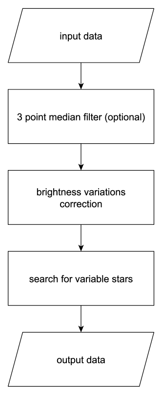
Figure 1: Structure of Astrokit program.

For the program to operate correctly, it also needs a file containing the equatorial coordinates of the stars. This file may also optionally contain the catalogued color indices which will be later taken into account when selecting ensembles of comparison stars.

Below we give a stage-by-stage description of the algorithm. Let the available set of photometric data consist of $j$ CCD frames each containing $i$ stars from the input catalog.

(1) The program computes the magnitudes (m) and magnitude errors (merr) for each star of the input catalog and each frame. These quantities are determined as follows:

$$\begin{array}[]{lcl}{\tt flux}&=&{\tt sum}-{\tt area}\times{\tt msky},\\[10.0pt] {\tt m}&=&{\tt zmag}-2.5\log({\tt flux})+2.5\log({\tt itime}),\\[10.0pt] {\tt merr}&=&\displaystyle\frac{1.0857}{{\tt flux}\times{\tt gain}}\,\Bigl{(}{\tt flux}\times{\tt gain}\\ \lx@intercol\@ADDCLASS{ltx_eqn_lefteqn}$\displaystyle+\,{\tt area}\,\bigl{(}1+{\tt area}/{\tt nsky}\bigr{)}\,\left({\tt msky}\times{\tt gain}+{\tt ron}^{2}\right)\Bigr{)}^{\frac{1}{2}}\!\!\!,$\mbox{}\hfil\lx@intercol&&\\[5.0pt] \end{array}$$ (1)

where ${\tt zmag}=20$ is the zero point of the magnitude scale; gain is the CCD gain in e^-/ADU, which is set by the user when beginning to work with the program; ron is the CCD readout noise in e^-/pixel, which is also set by the user.

(2) For each star from the input catalog, an ensemble of reference stars located within a certain radius (the default value is $5\arcmin$) is selected whose magnitudes differ from that of the star considered by no more than $2^{\rm m}$ (this parameter can be changed by the user). The smaller the magnitude difference, the smaller the number of stars in the ensemble, and the farther they are. Another criterion for selecting ensemble stars is based on the difference between the color index of the star considered (i.e., the star for which the ensemble is composed) and candidate comparison stars.

(3) The weighted average instrumental magnitude $\langle m_{j}\rangle$ of ensemble stars is computed for each frame of the series

$$\langle m_{j}\rangle=\frac{\sum\limits_{k}^{K}m_{kj}\,\omega_{k}}{\sum\limits_{k}^{K}\omega_{k}},\quad\mbox{where}\quad\omega_{k}=\frac{1}{\langle{\tt merr}_{k}^{2}\rangle},$$

where $k$ is the running number of the star in the ensemble, $K$ is the number of stars in the ensemble, $j$ is the frame number, $m_{kj}$ is the magnitude of $k$-th ensemble star in $j$-th frame, $\langle{\tt merr}_{k}\rangle$ is the mean theoretical error of measured magnitude $m_{k}$ of the ensemble star computed by formula (1) (instead of the error in each frame as in Everett & Howell (2001)).

(4) The mean magnitude $M$ of all ensemble stars averaged over all frames:

$$M=\frac{\sum\limits_{j}^{N}\langle m_{j}\rangle}{N},$$

where $N$ is the number of frames.

(5) The difference between the weighted average magnitude $\langle m_{j}\rangle$ of ensemble stars and the mean magnitude $M$ of all ensemble stars averaged over all frames is then subtracted from the observed magnitude of the star for which the effect of the terrestrial atmosphere is determined and for the ensemble stars:

$$m_{{\rm cor}\,ij}=m_{ij}-(\langle m_{j}\rangle-M),$$

where $m_{{\rm cor}\,ij}$ and $m_{ij}$ are respectively the corrected and initial magnitudes of star $i$ in frame $j$.

(6) After composing the initial ensemble, the standard deviation from the mean magnitude is computed for all stars, and the star with the greatest standard deviation is flagged. If the standard deviation from the mean magnitude is more than twice greater than the mean theoretical photometric error averaged over all frames (we call this the cutoff ratio of the sigma criterion), which can also be varied, the star is removed from the ensemble, and the procedure is repeated from step 2.

If after all stars with large standard deviations are removed the ensemble contains less than 10 stars, the size of the ensemble domain is increased by $1\arcmin$ and all the above steps are repeated. The correction of instrumental magnitudes is thus an iterative process, which is repeated until the ensemble contains more than nine stars or the search radius increases to $30\arcmin$.

The error introduced by the correction of the initial magnitudes using the ensemble stars is determined by the magnitude errors of the ensemble stars:

$${\tt merr}_{{\rm ens}}=\frac{1}{\sqrt{\sum\limits_{k=1}^{K}\displaystyle\frac{1}{{\tt merr}_{k}^{2}}}},$$

where ${\tt merr}_{k}$ is the measurement error for $k$-th star of the ensemble. The resulting error for star $i$ is composed of its measurement error and the error introduced by the comparison ensemble:

$${\tt merr}=\sqrt{{\tt merr}_{i}^{2}+{\tt merr}_{\rm ens}^{2}}.$$

The procedure of the formation of ensembles and the correction of instrumental magnitudes is performed for each star of the list. Thus, for each star its individual ensemble of closely located comparison stars is created.

Figure 2 shows schematically the process of the correction of instrumental magnitudes.

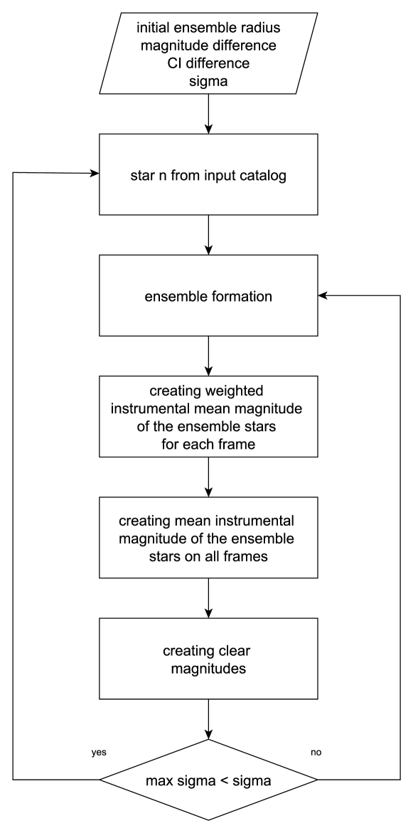
Figure 2: Flowchart of the process of the correction of instrumental magnitudes.

(7) Variable objects are identified by the algorithm described in Rose & Hintz (2007). For each star the coefficient ${\rm RoMS}$ (Robust Median Statistics) is computed:

$$\eta_{n}=\frac{\sum\limits_{i}\displaystyle\frac{\mid m_{i}-\langle m_{\rm med}\rangle\mid}{\sigma_{\rm rms}}}{N-1},$$

where $n$ is the number of a star; $m_{i}$ is the $i$-th measurement of the magnitude; $\langle m_{\rm med}\rangle$ is the median of magnitude measurements of star $n$; $N$ is the total number of magnitude measurements for star $n$; $\sigma_{\rm rms}$ is the estimated standard deviation of star $n$, determined by the least-squares method from the dependence of the standard deviations of the magnitude on the stellar magnitude for stars in the frame.

The ${\rm RoMS}$ criterion allows estimating the variations of the object brightness. If it exceeds $1$, the star is considered to be a suspected variable and is then analyzed more thoroughly.

3 Analysis of the technique

To analyze the technique and select the optimum input parameters for Astrokit to ensure the best photometric precision, we used the data of the photometric survey of a sky area in the Milky Way. A total of 3000 50-second $R$-band frames were taken with the MASTER-II-URAL telescope. In the central $30^{\prime}\times 30^{\prime}$ region of the frames, we selected 800 stars in the $R=9^{\rm m}$–$17^{\rm m}$ magnitude interval.

The MASTER-II-URAL is located at the Kourovka Observatory of the Ural Federal University. It is a Hamilton system twin telescope ($D=40$ cm, $F=1000$ cm) installed on equatorial mounting and equipped with two Apogee Alta U16M CCD cameras (Lipunov et al. (2010)). The image scale is $1\aas@@fstack{\prime\prime}8$/pixel. Photometric calibrations are performed using dark frames taken before each observing night and dawn flat-field frames. All observations are performed in automatic mode.

After performing aperture photometry with IRAF, we carried out a series of reduction cycles with Astrokit. We varied such input parameters as the initial radius $r$ of the ensemble, the magnitude difference $\Delta m$ and color-index difference $\Delta{\rm CI}$ of ensemble stars, and the cutoff ratio ($\sigma$) of the standard deviation of instrumental magnitude to the theoretical error (the sigma criterion).

We consider the main criterion characterizing the quality of post-processing to be the number of “good stars,​” i.e., stars with the standard deviation of magnitudes $s$ of less than $0\fmm 01$ and $0\fmm 02$ over the entire observing set. We also took into account the minimum computed standard deviation of magnitude for an individual star (hereafter the “best star”).

We first varied the initial radius of the ensemble with the magnitude difference fixed at $1^{\rm m}$ (shown by the squares in plots) and the sigma criterion equal to two. The initial ensemble radii were equal to $1^{\prime}$, $2^{\prime}$, $3^{\prime}$, $4^{\prime}$, $5^{\prime}$, $7^{\prime}$, $10^{\prime}$, and $15^{\prime}$. We then counted for each case the number of “good stars” and the minimum standard deviation for each initial radius.

As is evident from Fig. 3, the minimum standard deviation from the mean magnitude is equal to $0\fmm 00453$ for the initial radii from $1^{\prime}$ to $5^{\prime}$, increases with further increase of the ensemble radius, and reaches the maximum 5% difference ($0\fmm 00477$) for the ensemble radius of $15^{\prime}$.

The number of stars whose standard deviation from the mean magnitude over the entire observing set is less than $0\fmm 01$ reaches maximum at the ensemble radius of $7^{\prime}$: it is equal to 102 which is 7% greater than the corresponding number of stars for the initial ensemble radii from $1^{\prime}$ to $3^{\prime}$ (Fig. 4). The size of the subsample of stars with the standard deviation from the mean magnitude of less than $0\fmm 02$ reaches maximum at the initial ensemble radius of $10^{\prime}$ (254 stars compared to 245). The increment is equal to 4% (Fig. 5).

Figure 3: Variation of the standard deviation from the mean magnitude for the “best star” as a function of the initial ensemble radius for $\sigma=2$ and different $\Delta m$ values (the dependences for $\Delta m=1$ and $\Delta m=2$ are shown by the squares and triangles respectively).

Figure 4: Variation of the number of stars with the standard deviation from the mean magnitude of less than $0\fmm 01$ as a function of the initial ensemble radius for $\sigma=2$ and different $\Delta m$ values (the dependences for $\Delta m=1$ and $\Delta m=2$ are shown by the squares and triangles respectively).

Figure 5: Variation of the number of stars with the standard deviation from the mean magnitude of less than $0\fmm 02$ as a function of the initial ensemble radius for $\sigma=2$ and different $\Delta m$ values (the dependences for $\Delta m=1$ and $\Delta m=2$ are shown by the squares and triangles respectively).

Figure 6: Variation of the standard deviation from the mean magnitude for the “best star” (the top plot) and the number of stars with $s<0\fmm 01$ (the middle plot), $s<0\fmm 02$ (the bottom plot) as a function of the sigma criterion $\sigma$ for $r=5^{\prime}$ and $\Delta m=2$.

We similarly varied the initial ensemble radius with $\Delta m=2^{\rm m}$ (the corresponding curves in the figures are shown by the triangles). In this case the minimum standard deviation from the mean magnitude is $0\fmm 00446$ and also increases with initial radius (Fig. 3). The number of “good stars” with $s<0\fmm 01$ reaches maximum at the initial ensemble radii of $7^{\prime}$ and $10^{\prime}$ (it increases by 4%) (Fig. 4). The number of “good stars” with $s<0\fmm 02$ reaches maximum at the initial ensemble radius of $5^{\prime}$ (it increases by 4% compared to the minimum value) (Fig. 5).

In view of the above, we can conclude that the optimum initial radius of the ensemble of comparison stars is $5^{\prime}$–$7^{\prime}$ for the magnitude difference of $2^{\rm m}$. In this case the ensemble remains sufficiently compact while containing a large number of stars. The ensemble permits atmospheric effects to be reduced, and this reduction can be expressed in terms of the minimum standard deviation from the mean magnitude for the “best star” and the maximum number of “good stars.​” Note that the effect of the varied parameters on the final result is relatively small.

The next stage in the choice of the optimum parameters consisted in varying the sigma criterion with the initial radius and magnitude difference fixed at $5^{\prime}$ and $2^{\rm m}$ respectively.

As is evident from Fig. 6, the optimum value of the sigma criterion is equal to $2$. This can be explained by the fact that too “strict” value decreases the number of stars in the ensemble. A sigma criterion value greater than $2$ increases the number of stars in the ensemble by including stars with the greatest standard deviation from the mean magnitude over the entire observing set with inevitable effect on the final precision.

According to postulates of classical differential photometry with a single comparison star and control stars, the best precision can be achieved with a comparison star that is most similar to the object studied both in terms of brightness and spectral type. We studied the effect of color index on the precision of photometry. To this end, we varied the difference of the 2MASS $J-H$ color indices (Skrutskie et al. (2006)) when creating the ensemble of stars with the initial radius of $5^{\prime}$ and the magnitude difference of $2^{\rm m}$. We set the color-index difference equal to $0\fmm 1$, $0\fmm 2$, $0\fmm 3$, $0\fmm 4$, $0\fmm 5$, $0\fmm 6$, and $0\fmm 7$.

As is evident from Fig. 7, the closeness of stellar spectral types is not a necessary condition for achieving high precision. However, the classical approach of differential photometry remains the only solution in the case of small fields and insufficient number of stars for selecting an ensemble.

Figure 7: Variation of the standard deviation from the mean magnitude for the “best star” (the top plot) and the number of stars with $s<0\fmm 01$ (the middle plot), $s<0\fmm 02$ (the bottom plot) as a function of the color-index difference $\Delta{\rm CI}$ for $r=5^{\prime}$ and $\Delta m=2$.

Figure 8: Variation of the standard deviation from the mean magnitude for the “best star” (the top plot) and the number of stars with $s<0\fmm 01$ (the middle plot), $s<0\fmm 02$ (the bottom plot) as a function of the magnitude difference $\Delta m$ for $r=5^{\prime}$ and $\sigma=2$.

What will happen in the case if the ensemble contains the maximum possible number of reference stars? To this end, we varied the cutoff magnitude for the initial ensemble radius and sigma criterion equal to $5^{\prime}$ and $2$ respectively (Fig. 8).

Note that the $2^{\rm m}$ magnitude difference is optimal, because not all possible stars will make it into the ensemble if a smaller value is adopted. Adopting a magnitude difference greater than $2^{\rm m}$ would result in the inclusion into the ensemble the stars that are significantly brighter or fainter than the object studied, thereby degrading the final precision.

Our analysis leads us to conclude that in the case of the presence of a sufficient number of stars in the field, the best photometric precision is achieved using close ensembles with many stars. We thus have the following optimum parameter set for the formation of ensembles of comparison stars: the initial ensemble radius $r=5^{\prime}$–$7^{\prime}$, magnitude difference $\Delta m=2^{\rm m}$, and the cutoff ratio of the standard deviation from the mean magnitude to the theoretical error for the star to be included into the ensemble $\sigma=2$. Note that the closeness of the spectral types of stars is of no importance.

At the first sight, small variations in the number of “good stars” and the quality of the “best star” may appear insignificant and not to be worthy of efforts to find the optimum parameters. However, first, there is no harm in increasing the precision. Second, the number of “good stars” may increase significantly in the case of reduction of fields containing thousands of stars, and this may influence the number of candidates for searching for transits of “hot Jupiter” type exoplanets (e.g., if only stars with $s<0\fmm 02$ are selected).

4 Testing

Astrokit program is used for post reduction of photometric data obtained with wide-field telescopes of the MASTER robotic net. Below we report the results of its use for reducing a photometric survey of a Milky Way area in Cygnus, and the results of observations of the open cluster NGC 188 and the transit of the exoplanet WASP-11 b / HAT-P-10 b.

We reduced all data in accordance with the same procedure. We photometrically calibrated the CCD frames using dark-current and flat-field frames. We observed five dark frames for the particular set of exposures at dusk hours before observations. Each master dark frame for the particular exposure is made up of five frames via median stacking. We then subtract the master dark frame from the CCD frames with the object studied.

The flat-field frames in the filter considered are acquired automatically at dawn twilight with the telescope tracking turned off. The linear range of the CCDs employed is limited by 40 000 ADU, and therefore the exposure in each filter is chosen so that the number of counts in pixels would not exceed this limit. The master dark frame with the appropriate exposure is subtracted from each of the five flat-field frames. The flat-field frames are normalized (the count of each pixel is divided by the median count of all pixels), and then the master flat-field frame is computed as the median of the normalized initial flat-field frames. The CCD frames with the object studied are then divided by the resulting master flat-field frame. The use of flat-field frames allows pixel-to-pixel sensitivity variations and vignetting of the optical system to be taken into account.

After photometric calibration Astrometry.net application is used to write the correct astrometric-calibration (WCS) parameters to the FIST file header. Aperture photometry is then performed using IRAF PHOT/APPHOT task, and the results of this photometry serve as input data for Astrokit.

4.1 Photometric Survey in Cygnus

High-precision CCD observations were performed at the Kourovka Astronomical Observatory of the Ural Federal University from May through August 2012 within the framework of a pilot project aimed at the search for exoplanet transits and variable stars. A total of 3600 frames of of a $2\degr\times 2\degr$ area centered at $\alpha=20^{\rm h}30^{\rm m}00^{\rm s}$, $\delta=50\degr 30^{\prime}00^{\prime\prime}$ were acquired with the MASTER-II-URAL telescope, and the photometry of 21 500 stars was performed with a precision of $0\fmm 006$ to $0\fmm 5$ in the magnitude interval from $10^{\rm m}$ to $18^{\rm m}$. Figure 9 shows the standard deviation from the mean magnitude as a function of magnitude for the entire observing set. The right and left panels show the data before and after reduction with Astrokit.

Figure 9: Standard deviation from the mean magnitude as a function of magnitude for the entire observing set: the raw data (right) and the data after reduction with Astrokit (left).

As is evident from the figure, our program decreases the standard deviation from the mean magnitude by a factor of 10 for some stars.

With the ${\rm RoMS}=1$ threshold, Astrokit selected about 20% of all stars as candidate variables. A visual inspection of the light curves of the candidate variables allowed us to find 360 hitherto unknown variable stars including:

• 139 stars with periods longer than $20^{\rm d}$;

• 100 stars with periods ranging from $20^{\rm d}$ to $0\aas@@fstack{d}1$;

• 19 stars with periods shorter than $0\aas@@fstack{d}1$;

• 96 eclipsing variables;

• 5 flare stars;

• 1 dwarf nova.

Among the variables found was the outburst of the dwarf nova USNO-B1.0 1413-0363790 (Burdanov et al. (2012)). Several dozen variable stars were selected as candidate $\delta$ Sct stars. The brightness of the star was found to vary with an amplitude as small as $0\fmm 005$ (Fig. 10).

Figure 10: Phased light curve of the star 2MASS 20295743+5017071 with the period and amplitude of $0\fdd 035$ and $0\fmm 005$ respectively. The solid line shows the fitted data.

Other stars were found to exhibit periodic brightness decreases by $0\fmm 015$. These light variations may be due to transits of “hot Jupiter” type exoplanets with the radii of 1/10 of the radius of the host stars and orbiting with less than one day-long periods (Burdanov et al. (2013)).

4.2 Open Cluster NGC 188

The open cluster NGC 188 was observed in the $R$ and $I$ filters with the MASTER-II-URAL telescope over five nights in March 2011. A total of 400 frames were acquired, which were post-processed using Astrokit program. We performed aperture $R$-band photometry of 5513 stars with a precision ranging from $0\fmm 006$ to $0\fmm 05$ in a $1\aas@@fstack{\circ}5\times 1\aas@@fstack{\circ}5$ area. Although NGC 188 is a well-studied cluster (more than 500 papers in the past 50 years), our algorithm of the search for variable stars found 18 new variables (Popov et al. (2013)). Figure 11 shows the standard deviation from the mean magnitude as a function of magnitude after reduction by our program (left) and the ${\rm RoMS}$ coefficients for all stars (right). Variable stars are shown by the filled circles in both plots. As is evident from Fig. 11, the standard deviation from the mean magnitude for variables often does not differ from the corresponding standard deviations for constant stars, whereas the ${\rm RoMS}$ coefficient allows more confident selection of candidate variable objects.

Figure 11: Standard deviations from the mean magnitude (left) and coefficients ${\rm RoMS}$ (right) as a function of magnitude. The filled circles show variable stars.

4.3 Observations of Exoplanet Transits

During the transits of even the largest “hot Jupiters” moving in close orbits across the disk of the host star, its brightness dips by about $0\fmm 01$. To confidently record the very fact of transit and determine its duration and mid-time, in the case of such brightness dips the resulting photometry should have the precision of about $0\fmm 001$. Achieving the given precision is a difficult task for ground-based telescopes and requires special attention during differential photometry.

Below we compare the results obtained with Astrokit and the classical technique of differential photometry with a single comparison star, used to reduce the photometric observations of the transit of a “hot Jupiter” type exoplanet.

Our $R$-band observations of the transit of the exoplanet WASP-11 b / HAT-P-10 b ($R=11\fmm 01$, $J-H=0.46$, $H-K=0.14$) were made with the MASTER-II-Ural telescope on December 10, 2012.

The light curve of the transit was obtained using the classical method of differential photometry, with a single comparison star 3UC-242-019494 ($R=12^{\rm m}$, $J-H=0.55$, $H-K=0.125$), and a check star 3UC-242-019559 ($R=11\fmm 4$, $J-H=0.175$,$H-K=0.113$). These stars are located within less than $10^{\prime}$ from WASP-11/HAT-P-10 ($R=11\fmm 7$) and have close magnitudes and color indices. The light curve obtained from magnitude difference between WASP-11/HAT-P-10 and the comparison star is shown by the triangles in Fig. 12. The standard deviation of the magnitude difference between the comparison and control star was $0\fmm 006$.

Figure 12: $R$-band light curve of the exoplanet WASP-11 b / HAT-P-10 b transit. The light curve obtained with a single comparison star is shown by the triangles, and that obtained using an ensemble of comparison stars—by the squares (it is shifted for better visualization).

We used Astrokit program with an ensemble of 11 stars to correct photometry for atmospheric transparency variation. The stars are located within $6^{\prime}$ and their magnitudes differ by no more than $2^{\rm m}$ from that of the star studied. We estimate the precision of corrected photometry ($0\fmm 0039$) by the standard deviation from the mean magnitude for the control star 3UC-242-019559 mentioned above. The resulting precision is about a factor of 1.5 smaller that the standard deviation of the control-star magnitude in the case the classical method of differential photometry is used, thereby demonstrating the advantage of using ensembles of comparison stars. The resulting transit light curve is shown by the squares in Fig. 12.

This transit is remarkable by the fact that it was observed during total lunar eclipse. We clearly see that the scatter of data points increases toward the end of the transit. The standard deviation of the magnitude of the host star before the transit (the first 11 data points in the light curve) is equal to $0\fmm 002$ and begins to increase with increasing sky background due to the egress of the Moon out of the Earth shadow. The standard deviation of host-star magnitude after the transit (the last 11 data points) is four times greater and equal to $0\fmm 008$.

5 Conclusions

The use of a close ensemble of comparison stars while performing differential photometry allows the inhomogeneity of the data series, caused by local variations of atmospheric transparency and sky background, to be taken into account, and reduces the contribution of stellar scintillation to the error budget of the resulting magnitudes (Everett & Howell (2001); Kornilov (2012)). If more than 10 reference stars in a close ensemble are used, the difference between their spectral types and that of the object studied becomes unimportant. However, to achieve the best precision, the magnitude difference should be small (it should not exceed $2^{\rm m}$) and ensemble stars should be chosen within $5^{\prime}$–$7^{\prime}$ of the program star.

The resulting photometric precision after the application of Astrokit allows finding low-amplitude variables and study transits of “hot Jupiters.​”

The use of robust median statistics is approved because of its higher stability against outliers. However, it does not guarantee against finding false variables. A considerable part of suspected variables prove to be constant stars within the photometric errors after further analysis. The number of candidate variables is usually equal to about 10% of the total number of stars in the frame. The final criterion of the variability of a star is the visual inspection of its light curve.

The source code of the program is available at http://astro.ins.urfu.ru/en/node/1330.

Translated by A. Dambis