Abstract

The ground state of a homogeneous Bose gas of hard spheres is treated in self-consistent mean-field theory. It is shown that this approach provides an accurate description of the ground state of a Bose-Einstein condensed gas for arbitrarily strong interactions. The results are in good agreement with Monte Carlo numerical calculations. Since all other mean-field approximations are valid only for very small gas parameters, the present self-consistent theory is a unique mean-field approach allowing for an accurate description of Bose systems at arbitrary values of the gas parameter.

PACS: 03.75.Hh, 05.30.Ch, 05.30.Jp

1 Introduction

The quantum hard-sphere model serves as a reference or as an initial approximation for quantum systems with more complicated interaction potentials because this model is characterized only by a single interaction parameter composed of the system density and the sphere diameter. The interest to the hard-sphere Bose systems, initiated by the works of Bogolubov [1], Lee, Huang, and Yang [2-4], Wu [5], and others has been connected with the attempt to give a reasonable description for a quantum fluid with more realistic potentials, especially for liquid helium. By extensive numerical simulations, Kalos, Levesque, and Verlet [6] proved that the hard-sphere reference fluid is able to provide good description even for liquid helium, whose atoms interact through the Lennard-Jones potential. They showed that the attractive forces change the liquid structure only a little [6].

The model characterizing the interactions in Bose systems by a single gas parameter has become intensively employed for low-temperature Bose gases, where at small values of the gas parameter the system properties are shown to be universal, being almost independent on the particular shapes of interaction potentials [7]. Bose systems, whose atomic interactions are characterized by a gas parameter, have been extensively studied by Monte Carlo numerical calculations for both trapped [8-11] and homogeneous gases [7,12-14].

It would, certainly, be good to have a theory of a mean-field type, which could provide more or less simple formulas for treating Bose systems with finite gas parameters. However, there is a wide-spread consensus that there exist no theoretical description, based on a mean-field approximation, that could give reasonably accurate results outside of the region of very small gas parameters, where the Bogolubov approximation is valid. Actually, the Bogolubov approximation is often identified with the mean-field theory [7,9,12].

The absence for Bose-condensed systems of a mean-field approximation, that could give at low temperatures a reasonable description for finite or large interactions, seems rather strange, since for many other systems such mean-field approximations do exist. For example, many magnetic materials, defined by the Heisenberg or Ising models, at low temperatures can be reasonably well described by the mean-field approximation. Of course, a mean-field approximation can fail in the critical region or for reduced dimensions, but in three dimensions at very low temperatures, close to zero, such approximations do catch the main properties of magnetic materials [15,16].

In the present paper, we show that the low-temperature Bose systems are not outcasts enjoying no accurate mean-field theory, but there exists a mean-field approach providing a correct description of such systems for arbitrarily large gas parameters and yielding the results in close agreement with numerical Monte Carlo calculations.

2 Representative ensemble

Our consideration is based on the self-consistent approach to Bose-condensed systems [17-20], employing representative ensembles [21,22]. This approach guarantees the self-consistency of all thermodynamic relations, the validity of conservation laws, and a gapless spectrum of collective excitations.

The energy Hamiltonian for a Bose system of hard spheres is written in the standard form

$$\hat{H}=\int\hat{\psi}({\bf r})\left(-\;\frac{\nabla^{2}}{2m}\right)\hat{\psi}({\bf r})\;d{\bf r}\;+\;\frac{1}{2}\;\Phi_{0}\int\hat{\psi}^{\dagger}({\bf r})\hat{\psi}^{\dagger}({\bf r})\hat{\psi}({\bf r})\hat{\psi}({\bf r})\;d{\bf r}\;,$$ (1)

with the interaction strength

$$\Phi_{0}\equiv 4\pi\;\frac{a_{s}}{m}$$ (2)

characterized by scattering length $a_{s}$ and atomic mass $m$. The field operators satisfy the Bose commutation relations. Generally, the operators depend on time which, for brevity, is not shown explicitly. Here and in what follows, the Planck and Boltzmann constants are set to one.

Note that we take the interaction potential in the form of a local pseudopotential, which is admissible when the interaction radius is much shorter than mean interatomic distance. Strictly speaking, the scattering length represents the hard-sphere diameter only when the scattering length $a_{s}$ is essentially shorter than the interatomic spacing $a$. In that case, as is known [2-6,23], the results for the local pseudopotential coincide with those for the hard-sphere system. The use of the local pseudopotential for the finite values of the ratio $a_{s}/a$ can be justified by the following reasons. First of all, this ratio for a liquid cannot be larger than about $0.6$, since after this the liquid freezes [13]. More important is that the approximations we employ are based on the possibility of extrapolating the results obtained for small parameters to the large values of these parameters. Thus, the self-consistent mean-field approximation [18-20], we use, can be shown to be equivalent to a variational procedure with respect to atomic correlations, which makes it possible to extend the results from the region of weak interactions to that of strong interactions. The self-similar approximation allows us to extrapolate the expressions, derived in the limit of small coupling parameters, to the region of large parameters, as has been demonstrated for a number of quantum models [24,25]. These methods guarantee that the results obtained for the small ratio $a_{s}/a$, where $a_{s}$ well represents the hard-sphere diameter, provide us good approximations for the finite values of this ratio.

The necessary and sufficient condition for the occurrence of Bose-Einstein condensation is the spontaneous breaking of global gauge symmetry [26,27]. The symmetry breaking can be explicitly realized by means of the Bogolubov shift [28,29] for the field operator

$$\hat{\psi}({\bf r})=\eta({\bf r})+\psi_{1}({\bf r})\;,$$ (3)

where $\eta({\bf r})$ is the condensate wave function and $\psi_{1}(\bf r)$ is the field operator of uncondensed atoms. It is worth stressing that the Bogolubov shift (3) is not an approximation, but an exact canonical transformation [30].

To avoid double counting, the condensate function and the field operator of uncondensed atoms are assumed to be orthogonal to each other,

$$\int\eta^{*}({\bf r})\psi_{1}({\bf r})\;d{\bf r}=0\;.$$ (4)

The operator of uncondensed atoms on average is zero,

$$\langle\psi_{1}({\bf r})\rangle=0\;,$$ (5)

so that the condensate function plays the role of an order parameter

$$\eta({\bf r})=\langle\hat{\psi}({\bf r})\rangle\;.$$ (6)

By this definition, the condensate function and the field operator of uncondensed atoms are treated as separate variables [28,29], normalized, respectively, to the number of condensed atoms

$$N_{0}=\int|\;\eta({\bf r})\;|^{2}\;d{\bf r}$$ (7)

and to the number of uncondensed atoms

$$N_{1}=\langle\hat{N}_{1}\rangle\;,$$ (8)

where the operator of uncondensed atoms is

$$\hat{N}_{1}\equiv\int\psi^{\dagger}_{1}({\bf r})\psi_{1}({\bf r})\;d{\bf r}\;,$$

and the total number of atoms in the system is $N=N_{0}+N_{1}$.

The evolution equations for the variables are obtained [17,18,22] by the extremization of the effective action, under conditions (4) to (8), which yields the equation for the condensate function

$$i\;\frac{\partial}{\partial t}\;\eta({\bf r},t)=\left\langle\frac{\delta H}{\delta\eta^{*}({\bf r},t)}\right\rangle$$ (9)

and the equation for the operator of uncondensed atoms

$$i\;\frac{\partial}{\partial t}\;\psi_{1}({\bf r},t)=\frac{\delta H}{\delta\psi_{1}^{\dagger}({\bf r},t)}\;,$$ (10)

with the grand Hamiltonian

$$H=\hat{H}-\mu_{0}N_{0}-\mu_{1}\hat{N}_{1}-\hat{\Lambda}\;,$$ (11)

in which

$$\hat{\Lambda}=\int\left[\lambda({\bf r})\psi_{1}^{\dagger}({\bf r})+\lambda^{*}({\bf r})\psi_{1}({\bf r})\right]\;d{\bf r}\;.$$ (12)

The Lagrange multipliers $\mu_{0}$ and $\mu_{1}$ guarantee the validity of the normalization conditions (7) and (8), while the Lagrange multipliers $\lambda(\bf r)$ guarantee the conservation condition (5). These evolution equations are proved [31] to be identical to the Heisenberg equations of motion.

The system statistical operator in equilibrium is defined by minimizing the information functional [31,32] uniquely representing the system with the given restrictions. This results in the statistical operator

$$\hat{\rho}=\frac{1}{Z}\;e^{-\beta H}\qquad\left(Z\equiv{\rm Tr}e^{-\beta H}\right)\;,$$ (13)

with the same grand Hamiltonian (11) and $\beta\equiv 1/T$ being the inverse temperature.

For a system of $N$ atoms in volume $V$, the average density

$$\rho\equiv\frac{N}{V}=\rho_{0}+\rho_{1}$$ (14)

is the sum of the densities of condensed and uncondensed atoms, respectively,

$$\rho_{0}\equiv\frac{N_{0}}{V}\;,\qquad\rho_{1}\equiv\frac{N_{1}}{V}\;.$$ (15)

For a homogeneous system, $\eta(\bf r)=\sqrt{\rho_{0}}$. The terms, containing the operators of uncondensed atoms, are treated in the Hartree-Fock-Bogolubov approximation. The details of this self-consistent mean-field approach for Bose systems have been thoroughly exposed in Refs. [18-20,22,31], so that here we omit the intermediate calculations, passing to the final results. For the density of uncondensed atoms, we find

$$\rho_{1}=\int\left[\frac{\omega_{k}}{2\varepsilon_{k}}\;\coth\left(\frac{\varepsilon_{k}}{2T}\right)-\;\frac{1}{2}\right]\;\frac{d{\bf k}}{(2\pi)^{3}}\;,$$ (16)

where the notation

$$\omega_{k}\equiv\frac{k^{2}}{2m}+mc^{2}$$ (17)

is used, and the expression

$$\varepsilon_{k}=\sqrt{(ck)^{2}+\left(\frac{k^{2}}{2m}\right)^{2}}$$ (18)

represents the spectrum of collective excitations. The sound velocity $c$ is defined by the equation

$$mc^{2}=(\rho_{0}+\sigma_{1})\Phi_{0}\;.$$ (19)

The anomalous average

$$\sigma_{1}=-\int\frac{mc^{2}}{2\varepsilon_{k}}\coth\left(\frac{\varepsilon_{k}}{2T}\right)\;\frac{d{\bf k}}{(2\pi)^{3}}$$ (20)

describes the density $|\sigma_{1}|$ of pair-correlated atoms [31].

3 Zero temperature

To consider the ground state, we set temperature to zero. Then the density of uncondensed atoms (16) becomes

$$\rho_{1}=\frac{(mc)^{3}}{3\pi^{2}}\qquad(T=0)\;,$$ (21)

while for the anomalous average, we have

$$\sigma_{1}=-mc^{2}\int\frac{1}{2\varepsilon_{k}}\;\frac{d{\bf k}}{(2\pi)^{3}}\;.$$ (22)

This integral (22) for the anomalous average is divergent. This is why the often used practice is to omit the anomalous average at all, just setting $\sigma_{1}$ to zero. This, however, is principally wrong, since the nonzero anomalous average is the manifestation of the broken gauge symmetry, in the same way as the nonzero condensate fraction. Omitting the former would require to neglect the latter, hence, would prohibit the condensate existence. It is straightforward to show that neglecting the anomalous average makes the system with Bose-Einstein condensate unstable [17,22,31,33].

The integral (22) can be regularized by invoking one of the known regularization procedures, all of which are actually equivalent to the dimensional regularization [34]. Such a regularization is known to be asymptotically exact in the limit of weak interactions. Therefore, regularizing the integral in Eq. (22), one has to keep in mind the limit $\Phi_{0}\rightarrow 0$ in the spectrum (18), which can be taken into account by replacing there $c$ with $c_{eff}$, such that

$$c_{eff}\simeq c_{B}\qquad(\Phi_{0}\rightarrow 0)\;,$$ (23)

where

$$c_{B}\equiv\sqrt{\frac{\rho}{m}\;\Phi_{0}}$$ (24)

is the asymptotic value of the sound velocity for $\Phi_{0}\rightarrow 0$, that is, the Bogolubov sound velocity [1,28,29]. This yields

$$\int\frac{1}{2\varepsilon_{k}}\;\frac{d{\bf k}}{(2\pi)^{3}}=-\;\frac{m^{2}}{\pi^{2}}\;c_{eff}\;.$$ (25)

Thus, the anomalous average (22) can be reduced to the form

$$\sigma_{1}=\frac{m^{3}c^{2}}{\pi^{2}}\;c_{eff}\qquad(\Phi_{0}\rightarrow 0)$$ (26)

that is asymptotically exact in the limit of weak interactions [34].

Since we are interested in describing finite values of atomic interactions, the next step would be an analytic continuation of form (26) to finite $\Phi_{0}$. Before defining this procedure, let us pass to dimensionless quantities that will also be more convenient for numerical calculations.

Let us define the fractions of condensed and uncondensed atoms, respectively,

$$n_{0}\equiv\frac{\rho_{0}}{\rho}\;,\qquad n_{1}\equiv\frac{\rho_{1}}{\rho}\;,$$ (27)

and the dimensionless anomalous average

$$\sigma=\frac{\sigma_{1}}{\rho}\;.$$ (28)

And let us introduce the dimensionless sound velocity

$$s\equiv\frac{mc}{\rho^{1/3}}\;.$$ (29)

As a dimensionless strength of atomic interactions, it is natural to use the gas parameter

$$\gamma\equiv\rho^{1/3}a_{s}\;,$$ (30)

which is of order of the ratio $a_{s}/a$.

It is worth emphasizing that this parameter is natural, since it describes the ratio of the effective potential energy of an atom to its kinetic energy. Really, potential energy per atom is proportional to $\rho a_{s}/m$, while kinetic energy is of order $\rho^{2/3}/m$. The ratio of the former to the latter gives exactly the gas parameter (30).

In the dimensionless units, the fraction of uncondensed atoms reads as

$$n_{1}=\frac{s^{3}}{3\pi^{2}}\;.$$ (31)

Equation (19) for the sound velocity transforms into

$$s^{2}=s_{B}^{2}(n_{0}+\sigma)\;,$$ (32)

with the dimensionless Bogolubov velocity

$$s_{B}\equiv\frac{mc_{B}}{\rho^{1/3}}=\sqrt{4\pi\gamma}\;.$$ (33)

The equation for the anomalous average (26) reduces to

$$\sigma=\frac{s^{2}}{\pi^{2}}\;s_{eff}\qquad(\gamma\rightarrow 0)\;,$$ (34)

where $s_{eff}=mc_{eff}/\rho^{1/3}$.

The problem in extending the weak-interaction formula (34) to finite interactions is the necessity of defining an analytic continuation from asymptotically small $\gamma\rightarrow 0$ to the finite values of $\gamma$. Such an analytic continuation seems to be not uniquely defined. For instance, if we set $s_{eff}=s_{B}$ in Eq. (34), we come back to a Bogolubov-type approximation that can be accurate for small gas parameters $\gamma<0.1$. Setting $s_{eff}=s$, we get the approximation of Ref. [35], valid for $\gamma<0.2$.

In order to extend the validity of approximations to larger values of $\gamma$, it is useful to keep in mind that, as has been stressed above, the nonzero anomalous average requires a nonzero condensate fraction, as far as both of them arise due to the global gauge symmetry breaking occurring under Bose-Einstein condensation [26,27]. On the contrary, the zero condensate fraction implies the zero anomalous average, which writes as the condition

$$\sigma\rightarrow 0\qquad(n_{0}\rightarrow 0)\;.$$ (35)

The mentioned approximations $s_{eff}=s_{B}$ and $s_{eff}=s$ do not satisfy condition (35), which explains why they do not allow for extending expression (34) to the values of the gas parameter larger than $\gamma<0.2$.

An approximation, satisfying condition (35), can be obtained by defining $s_{eff}$ from Eq. (32) by setting $\sigma$ to zero in the right-hand side of this equation, which gives $s_{eff}=\sqrt{4\pi\gamma n_{0}}$. This approximation was employed in Ref. [19], which allowed for the extension of the accurate results to $\gamma<0.4$, as compared with the Monte Carlo calculations [7,13].

Now we propose a better justified procedure for analytically extending the anomalous average to higher values of the gas parameter. For this purpose, we rewrite Eqs. (32) and (34) in the form of the iterative equations

$$s^{(n+1)}=s_{B}\;\sqrt{n_{0}+\sigma^{(n)}}\;,\qquad\sigma^{(n+1)}=\frac{s_{B}^{2}}{\pi^{2}}\;s^{(n+1)}\;,$$ (36)

in which $n$ is an iteration number. Notice that these equations can be combined into one iterative relation

$$\sigma^{(n+1)}=\frac{s_{B}^{3}}{\pi^{2}}\;\;\sqrt{n_{0}+\sigma^{(n)}}\;.$$ (37)

The Bogolubov approximation, with $s^{(0)}=s_{B}$ and $\sigma^{(0)}=0$ can be accepted as the zero-order approximation for the iterative procedure. Then the first iteration gives

$$s^{(1)}=s_{B}\;\sqrt{n_{0}}\;,\qquad\sigma^{(1)}=\frac{s_{B}^{3}}{\pi^{2}}\;\sqrt{n_{0}}\;.$$ (38)

This is equivalent to the approximation of Ref. [19] that, hence, can be considered as the first iteration of the iterative procedure. To second order, we obtain

$$s^{(2)}=s_{B}\left(n_{0}+\frac{s_{B}^{3}}{\pi^{2}}\;\sqrt{n_{0}}\right)^{1/2}\;,\qquad\sigma^{(2)}=\frac{s_{B}^{3}}{\pi^{2}}\;\left(n_{0}+\frac{s_{B}^{3}}{\pi^{2}}\;\sqrt{n_{0}}\right)^{1/2}\;.$$ (39)

In what follows, we shall use the second-order iteration for $\sigma$.

Summarizing the above consideration, we thus come to the system of equations

$$n_{0}=1-n_{1}\;,\qquad n_{1}=\frac{s^{3}}{3\pi^{2}}\;,$$

$$s^{2}=s_{B}^{2}(n_{0}+\sigma)\;,$$

$$\sigma=\frac{s_{B}^{3}}{\pi^{2}}\;\left(n_{0}+\frac{s_{B}^{3}}{\pi^{2}}\;\sqrt{n_{0}}\right)^{1/2}\;,$$ (40)

self-consistently defining the condensate fraction $n_{0}$, fraction of uncondensed atoms $n_{1}$, sound velocity $s$, and the anomalous average $\sigma$.

At small gas parameter $\gamma\rightarrow 0$, we have

$$n_{0}\simeq 1-\;\frac{8}{3\sqrt{\pi}}\;\gamma^{3/2}\;-\;\frac{64}{3\pi}\;\gamma^{3}\;-\frac{256}{9\pi^{3/2}}\;\gamma^{9/2}\;,$$

$$n_{1}\simeq\frac{8}{3\sqrt{\pi}}\;\gamma^{3/2}\;+\;\frac{64}{3\pi}\;\gamma^{3}\;+\;\frac{256}{9\pi^{3/2}}\;\gamma^{9/2}\;,$$

$$s\simeq\sqrt{4\pi\gamma}\>+\;\frac{16}{3}\;\gamma^{2}\;-\;\frac{64}{9\sqrt{\pi}}\;\gamma^{7/2}-\frac{4480}{27\pi}\;\gamma^{5}\;,$$

$$\sigma\simeq\frac{8}{\sqrt{\pi}}\;\gamma^{3/2}\;+\;\frac{64}{3\pi}\;\gamma^{3}\;-\;\frac{1408}{9\pi^{3/2}}\;\gamma^{9/2}\;.$$

The first two terms in the expansion for the condensate fraction $n_{0}$ exactly reproduce the Bogolubov behavior of $n_{0}$. We may notice that the anomalous average is larger than the fraction of uncondensed atoms $n_{1}$, in particular

$$\lim_{\gamma\rightarrow 0}\;\frac{\sigma}{n_{1}}=3\;.$$

It is, therefore, would be mathematically incorrect to neglect $\sigma$ leaving the three times smaller quantity $n_{1}$. The anomalous average is an important quantity, without which the description would not be self-consistent and the system would be unstable.

The behavior at large $\gamma$ can also be found from Eqs. (40). However, strictly speaking, considering $\gamma\gg 1$ is not applicable to a stable system, since it freezes at $\gamma=0.653$, as follows from the Monte Carlo simulations [13]. But, keeping in mind a metastable situation, we can formally study large values of $\gamma\gg 1$, which leads to

$$n_{0}\simeq 4\times 10^{-5}\;\frac{1}{\gamma^{13}}\;,\qquad n_{1}=1-n_{0}\;,$$

$$s\simeq(3\pi^{2})^{1/3}-\left(\frac{\pi}{3}\right)^{2/3}\;n_{0}\;,\qquad\sigma\simeq\frac{(9\pi)^{1/3}}{4}\;\frac{1}{\gamma}\;-\;n_{0}\;.$$

In the case of cold trapped atoms, although the scattering length can be made very large by means of Feshbach resonance, but such gases become unstable with respect to three-body recombination leading to significant particle loss and heating [36].

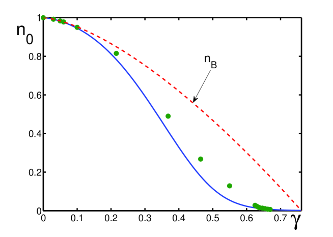
Figure 1: Condensate fraction $n_{0}$ (solid line) as a function of the gas parameter $\gamma$, compared with the Monte Carlo results by Rossi and Salasnich [13], shown by dots, and with the Bogolubov approximation $n_{B}$ (dashed line). The latter is not applicable above $\gamma=0.1$.

We solve Eqs. (40) for arbitrary values of the gas parameter $\gamma$ and compare our results with the Monte Carlo simulations by Rossi and Salasnich [13]. The latter confirm the earlier Monte Carlo calculations [7] and provide essentially more information for the larger values of the gas parameter. In Fig. 1, the behavior of the condensate fraction $n_{0}$ is shown, demonstrating good agreement with the Monte Carlo simulations [13] in the whole range of $\gamma$. The Bogolubov expression for the condensate fraction

$$n_{B}=1\;-\;\frac{8}{3\sqrt{\pi}}\;\gamma^{3/2}$$

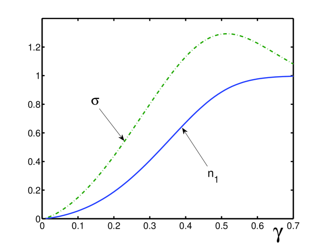
Figure 2: Fraction of uncondensed atoms $n_{1}$ (solid line) and anomalous average $\sigma$ (dashed-dotted line) as functions of the gas parameter $\gamma$. The anomalous average is everywhere larger than the $n_{1}$.

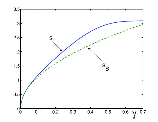
Figure 3: Sound velocity $s$ (solid line) in dimensionless units, compared with the Bogolubov sound velocity $s_{B}$ (dashed line), as functions of $\gamma$. The Bogolubov approximation essentially deviates from $s$ above $\gamma=0.1$.

is also shown. As is evident, $n_{B}$ gives a good approximation only for $\gamma<0.1$ and for larger $\gamma$ is not applicable, deviating too strongly from the numerical data. Figure 2 presents the fraction of uncondensed atoms $n_{1}$ and the anomalous average $\sigma$. As is seen, the latter is larger than the former in the whole range of the considered $\gamma$. In Fig. 3, the dimensionless sound velocity $s$ is compared with the Bogolubov sound velocity $s_{B}$. The former is larger than the latter, although their values are close to each other.

There have been a number of attempts to measure the condensate fraction in superfluid ⁴He with different experiments [37-41]. The estimated values of $n_{0}$ at zero temperature are in the range between $2\%$ and $10\%$. The most recent rather precise experiments [42-44] give the zero temperature value $n_{0}=(7.25\pm 0.75)\%$ at saturated vapor pressure and $n_{0}=(2.8\pm 0.2)\%$ at the pressure close to solidification. The latter value has also been confirmed by the diffusion Monte Carlo calculations [44]. The atoms of ⁴He at saturated vapor pressure can be well represented [6] by hard spheres of diameter $a_{s}=2.203$ Å, which corresponds to the gas parameter $\gamma=0.59$. At this value, we get the condensate fraction about $3\%$.

4 Ground-state energy

The system ground-state energy is the internal energy at zero temperature

$$E=\langle\hat{H}\rangle\qquad(T=0)\;.$$ (41)

It is customary to express this energy in units of $\hbar^{2}/2ma_{s}^{2}$. In our notation, this gives the dimensionless ground-state energy

$$E_{0}\equiv 2ma_{s}^{2}\;\frac{E}{N}\;.$$ (42)

Calculating the energy, we meet the divergent integral

$$\int(\varepsilon_{k}-\omega_{k})\;\frac{d{\bf k}}{(2\pi)^{3}}=\frac{16m^{4}}{15\pi^{2}}\;c_{eff}^{5}\;,$$

which is again regularized invoking dimensional regularization [31]. Then for small gas parameters, we have

$$E_{0}=4\pi\gamma^{3}\left(1+n_{1}^{2}-2n_{1}\sigma-\sigma^{2}+\frac{4s_{eff}^{5}}{15\pi^{3}\gamma}\right)\;,$$ (43)

which yields the asymptotic, as $\gamma\rightarrow 0$, expansion

$$E_{0}(\gamma)\simeq 4\pi\gamma^{3}\left(1+\frac{128}{15\sqrt{\pi}}\;\gamma^{3/2}+\frac{128}{9\pi}\;\gamma^{3}\;-\;\frac{2048}{9\pi^{3/2}}\;\gamma^{9/2}\right)\;.$$ (44)

The first two terms in the right-hand side of Eq. (44) exactly coincide with the Lee-Huang-Yang formula [2-4]. The simplest way for extending this expression to the larger values of the gas parameter is to use the extrapolation procedure based on self-similar factor approximants [25]. To second order, we find

$$E_{0}(\gamma)=4\pi\gamma^{3}(1+2.93379\gamma^{3/2})^{1.64103}\;.$$ (45)

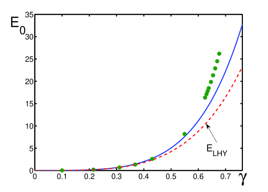
Figure 4: Dimensionless ground-state energy $E_{0}$ (solid line) as a function of the gas parameter $\gamma$, compared with the Monte Carlo results by Rossi and Salasnich [13], shown by dots, and with the Lee-Huang-Yang expression $E_{LHY}$ (dashed line). The latter deviates from the numerical data after $\gamma=0.4$.

This formula for $\gamma\ll 1$ reproduces exactly the Lee-Huang-Yang expression [2-4]. The behavior of the ground-state energy (45) is shown in Fig. 4, compared with the Monte Carlo calculations by Rossi and Salasnich [13] and with the Lee-Huang-Yang perturbative expression

$$E_{LHY}=4\pi\gamma^{3}\left(1+\frac{128}{15\sqrt{\pi}}\;\gamma^{3/2}\right)\;.$$

The agreement of our results with the Monte Carlo data [13] is good up to the values $\gamma\approx 0.6$. Let us recall that, actually, the system freezes [13] at $\gamma\approx 0.65$, so that to consider the gas parameters larger than the freezing value $0.65$ is not of much meaning. Let us emphasize that expression (45) has been obtained without any fitting. The Lee-Huang-Yang values of $E_{LHY}$ give a good approximation only for $\gamma<0.4$, while our formula (45) yields the values practically coinciding with the Monte Carlo Data [13] up to $\gamma=0.6$.

5 Conclusion

We have considered the ground state of a homogeneous Bose-condensed gas with a local pseudopotential imitating the hard-sphere interactions. The consideration is based on self-consistent mean-field approximation developed earlier by the authors. This approach allows one to extend the results obtained for small gas parameters to finite values of the latter. It is shown to be in good agreement with the accurate Monte Carlo results by Rossi and Salasnich [13] for all finite values of the gas parameter between zero and the point of freezing. The importance of using a correct expression for the anomalous average is emphasized. This explains why the previously used approximations could not provide sufficiently accurate behavior of the condensate fraction for finite gas parameters.

The main difference of the present paper from our previous publications is that here we have suggested an interative procedure for defining the anomalous average. The zeroth iteration of this procedure corresponds to the Bogolubov approximation, where the anomalous average is zero. This approximation is reasonable for small gas parameters $\gamma<0.1$, but is not applicable for larger values of $\gamma$, as is evident from the comparison in the figures.

The first iteration (38) corresponds to the expression we used in our earlier papers, which extends the applicability of the results to $\gamma\approx 0.4$. However, for the gas parameter larger than $0.4$, our previous results do not provide good approximation, as has been thoroughly analyzed in the paper by Rossi and Salasnich [13].

Now we have employed the second-order iteration (39), which have allowed us to essentially improve the results, making them very close to the numerical Monte Carlo data, as is demonstrated in the presented figures.

Recently, we have demonstrated [45] that the self-consistent mean-field approach is the sole mean-field theory correctly describing Bose-Einstein condensation as a phase transition of second order for arbitrary values of the gas parameter. Now we have also proved that this approach provides quite accurate approximations for the condensate fraction and ground-state energy of the Bose system, being in good agreement with numerical Monte Carlo data [13].

Acknowledgments

The authors are grateful to L. Salasnich for useful discussions and for the detailed information on the data of his Monte Carlo calculations. Financial support from the Russian Foundation for Basic Research (grant $\#14-02-00723$) is appreciated.

Figure Captions

Figure 1. Condensate fraction $n_{0}$ (solid line) as a function of the gas parameter $\gamma$, compared with the Monte Carlo results by Rossi and Salasnich [13], shown by dots, and with the Bogolubov approximation $n_{B}$ (dashed line). The latter is not applicable above $\gamma=0.1$.

Figure 2. Fraction of uncondensed atoms $n_{1}$ (solid line) and anomalous average $\sigma$ (dashed-dotted line) as functions of the gas parameter $\gamma$. The anomalous average is everywhere larger than the $n_{1}$.

Figure 3. Sound velocity $s$ (solid line) in dimensionless units, compared with the Bogolubov sound velocity $s_{B}$ (dashed line), as functions of $\gamma$. The Bogolubov approximation essentially deviates from $s$ above $\gamma=0.1$.

Figure 4. Dimensionless ground-state energy $E_{0}$ (solid line) as a function of the gas parameter $\gamma$, compared with the Monte Carlo results by Rossi and Salasnich [13], shown by dots, and with the Lee-Huang-Yang expression $E_{LHY}$ (dashed line). The latter deviates from the numerical data after $\gamma=0.4$.

References

- [1] N.N. Bogolubov, J. Phys. (Moscow) 11, 23 (1947).
- [2] T.D. Lee and C.N. Yang, Phys. Rev. 105, 1119 (1957).
- [3] T.D. Lee, K. Huang, and C.N. Yang, Phys. Rev. 106, 1135 (1957).
- [4] T.D. Lee and C.N. Yang, Phys. Rev. 112, 1419 (1958).
- [5] T.T. Wu, Phys. Rev. 115, 1390 (1959).
- [6] M.H. Kalos, D. Levesque, and L. Verlet, Phys. Rev. A 9, 2178 (1974).
- [7] S. Giorgini, J. Boronat, and J. Casulleras, Phys. Rev. A 60, 5129 (1999).
- [8] J.L. DuBois and H.R. Glyde, Phys. Rev. A 63, 023602 (2001).
- [9] J.L. DuBois and H.R. Glyde, Phys. Rev. A 68, 033602 (2003).
- [10] W. Purwanto and S. Zhang, Phys. Rev. A 72, 053610 (2005).
- [11] K. Nho and D.P. Landau, Phys. Rev. A 73, 033606 (2006).
- [12] N. Navon, S. Piatecki, K. Günter, B. Rem, T.C. Nguyen, F. Chevy, W. Krauth, and C. Salomon, Phys. Rev. Lett. 107, 135301 (2011).
- [13] M. Rossi and L. Salasnich, Phys. Rev. A 88, 053617 (2013).
- [14] M. Rossi, L. Salasnich, P. Ancilotto, and F. Toigo, Phys. Rev. A 89, 041602 (2014).
- [15] V.I. Yukalov and A.S. Shumovsky, Lectures on Phase Transitions (World Scientific, Singapore, 1990).
- [16] J.M.D. Coey, Magnetism and Magnetic Materials (Cambridge University, Cambridge, 2010).
- [17] V.I. Yukalov, Phys. Rev. E 72, 066119 (2005).
- [18] V.I. Yukalov, Phys. Lett. A 359, 712 (2006).
- [19] V.I. Yukalov and E.P. Yukalova, Phys. Rev. A 74, 063623 (2006).
- [20] V.I. Yukalov and E.P. Yukalova, Phys. Rev. A 76, 013602 (2007).
- [21] V.I. Yukalov, Phys. Rep. 208, 395 (1991).
- [22] V.I. Yukalov, Ann. Phys. (N.Y.), 323, 461 (2008).
- [23] K. Huang, C.N. Yang, and J.M. Luttinger, Phys. Rev. 105, 776 (1957).
- [24] V.I. Yukalov and E.P. Yukalova, Ann. Phys. (N.Y.) 277, 219 (1999).
- [25] V.I. Yukalov and E.P. Yukalova, Phys. Lett. A 368, 341 (2007).
- [26] E.H. Lieb, R. Seiringer, J.P. Solovej, and J. Yngvason, The Mathematics of the Bose Gas and Its Condensation (Birkhäuser, Basel, 2005).
- [27] V.I. Yukalov, Laser Phys. Lett. 4, 632 (2007).
- [28] N.N. Bogolubov, Lectures on Quantum Statistics (Gordon and Breach, New York, 1967), Vol. 1.
- [29] N.N. Bogolubov, Lectures on Quantum Statistics (Gordon and Breach, New York, 1970), Vol. 2.
- [30] V.I. Yukalov, Laser Phys. 16, 511 (2006).
- [31] V.I. Yukalov, Phys. Part. Nucl. 42, 460 (2011).
- [32] V.I. Yukalov, Laser Phys. 23, 062001 (2013).
- [33] A. Rakhimov, C.K. Kim, S.H. Kim, and J.H. Yee, Phys. Rev. A 77, 033626 (2008).
- [34] J.O. Andersen, Rev. Mod. Phys. 76, 599 (2004).
- [35] V.I. Yukalov and H. Kleinert, Phys. Rev. A 73, 063612 (2006).
- [36] R.J. Fletcher, A.I. Gaunt, N. Navon, R.P. Smith, and Z. Hadzibabic, Phys. Rev. Lett. 111, 125303 (2013).
- [37] H.A. Mook, R. Schern, and M.K. Wilkinson, Phys. Rev. A 6, 2268 (1972).
- [38] F.H. Wirth and R.B. Hallock, Phys. Rev. B 35, 89 (1987).
- [39] T.R. Sosnick, W.M. Snow, and P.E. Sokol, Phys. Rev. B 41, 707 (1990).
- [40] R.T. Azuah, W.G. Stirling, H.R. Glyde, M. Boninsegni, P.E. Sokol, and S.M. Bennington, Phys. Rev. B 56, 14620 (1997).
- [41] A.S. Rinat and M.F. Taragin, J. Low. Temp. Phys. 123, 139 (2001).
- [42] H.R. Glyde, R.T. Azuah, and W.G. Stirling, Phys. Rev. B 62, 14337 (2000).
- [43] H.R. Glyde, S.O. Diallo, R.T. Azuah, O. Kirichek, and J.W. Taylor, Phys. Rev. B 84, 184506 (2011).
- [44] S.O. Diallo, R.T. Azuah, D.L. Abernathy. R. Rota, J. Boronat, and H.R. Glyde, Phys. Rev. B 85, 140505 (2012).
- [45] V.I. Yukalov and E.P. Yukalova, J. Phys. B 47, 095302 (2014).