Mott transition in cuprate high-temperature superconductors

Abstract

In this study, we investigate the metal-insulator transition of charge transfer type in high-temperature cuprates. We first show that we must introduce a new band parameter in the three-band d-p model to reproduce the Fermi surface of high temperature cuprates such as BSCCO, YBCO and Hg1201. We present a new wave function of a Mott insulator based on the improved Gutzwiller function, and show that there is a transition from a metal to a charge-transfer insulator for such parameters by using the variational Monte Carlo method. This transition occurs when the level difference $\Delta_{dp}\equiv\epsilon_{p}-\epsilon_{d}$ between d and p orbitals reaches a critical value $(\Delta_{dp})_{c}$. The energy gain $\Delta E$, measured from the limit of large $\Delta_{dp}$, is proportional to $1/\Delta_{dp}$ for $\Delta_{dp}>(\Delta_{dp})_{c}$: $\Delta E\propto-t_{dp}^{2}/\Delta_{dp}$. We obtain $(\Delta_{dp})_{c}\simeq 2t_{dp}$ using the realistic band parameters.

Introduction The study of high-temperature superconductors has been intensively addressed since the discovery of cuprate high-temperature superconductors. The research of mechanism of superconductivity (SC) in high-temperature superconductors has attracted much attention and has been extensively studied using various models. It has been established that the Cooper pairs of high-temperature cuprates have the $d$-wave symmetry in the hole-doped materialsben03 . Therefore the electron correlation plays an important and the CuO₂ plane in cuprates plays a key role for the appearance of superconductivityzaa85 ; hir89 ; sca91 ; gue98 . The three-band d-p model is the most fundamental model for high-temperature cuprateshir89 ; sca91 ; gue98 ; koi00 ; yan01 ; yan08 ; yan09 ; web09 ; lau11 ; yan13 .

The purpose of this paper is to investigate the effect of electron correlation in the half-filled case, that is, to discuss the metal-insulator transition due to the on-site Coulomb repulsion. As was discussed in Ref.zaa85 , insulators are classified in terms of charge-transfer insulator or Mott insulator. The cuprates belong to the class of charge-transfer insulators. When the level difference $\Delta_{dp}\equiv\epsilon_{p}-\epsilon_{d}$ between $d$ and $p$ orbitals is large, the ground state will be insulating when the Coulomb repulsion $U_{d}$ on copper sites is large. (In this paper, we use the hole picture.) When $U_{d}$ is large, there will be a transition form a metal to an insulator as $\Delta_{dp}$ is increased. This is the Mott transition of charge-transfer type.

We will investigate this transition by using a variational Monte Carlo (VMC) method. In correlated electron systems, we must take into account the electron correlation correctly. Using the VMC method we can treat the electron systems properly from weakly to strongly correlated regions. We propose a wave function for an insulator on the basis of the Gutzwiller ansatz and examine the ground state within the space of variational functions. The expectation values are evaluated by using the variational Monte Carlo algorithmgro87 ; yok87 ; nak97 ; yam98 ; yam00 ; miy04 .

We first discuss the Mott state of the single-band Hubbard model by proposing a Mott-state wave function. We show that there is a metal-insulator transition as the on-site Coulomb repulsion $U$ is increased. The energy gain, compared to the limit of large $U$, is proportional to the exchange interaction $J\equiv 4t^{2}/U$ in the insulating state. The wave function is generalized straightforwardly to the d-p model. In the localized region, where $\Delta_{dp}$ is greater than the critical value $(\Delta_{dp})_{c}$, the energy gain $\Delta E$ is proportional to $-1/\Delta_{dp}$, that is, $\Delta E\propto-t_{dp}^{2}/\Delta_{dp}$. In this region we have the insulating ground state. $(\Delta_{dp})_{c}$ is of the order of the transfer integral $t_{dp}$ between holes in adjacent copper and oxygen atoms. This value is consistent with the result obtained by the dynamical mean-field theoryweb08 .

Hamiltonian The three-band model that explicitly includes oxygen p and copper d orbitals contains the parameters $U_{d}$, $U_{p}$, $t_{dp}$, $t_{pp}$, $\epsilon_{d}$ and $\epsilon_{p}$. The Hamiltonian is written as

$$H_{dp} = \epsilon_{d}\sum_{i\sigma}d_{i\sigma}^{{\dagger}}d_{i\sigma}+\epsilon_{p}\sum_{i\sigma}(p_{i+\hat{x}/2\sigma}^{{\dagger}}p_{i+\hat{x}/2\sigma}$$ (1)

$$+ p_{i+\hat{y}/2\sigma}^{{\dagger}}p_{i+\hat{y}/2\sigma})$$

$$+ t_{dp}\sum_{i\sigma}[d_{i\sigma}^{{\dagger}}(p_{i+\hat{x}/2\sigma}+p_{i+\hat{y}/2\sigma}-p_{i-\hat{x}/2\sigma}-p_{i-\hat{y}/2\sigma})$$

$$+ {\rm h.c.}]$$

$$+ t_{pp}\sum_{i\sigma}[p_{i+\hat{y}/2\sigma}^{{\dagger}}p_{i+\hat{x}/2\sigma}-p_{i+\hat{y}/2\sigma}^{{\dagger}}p_{i-\hat{x}/2\sigma}$$

$$- p_{i-\hat{y}/2\sigma}^{{\dagger}}p_{i+\hat{x}/2\sigma}+p_{i-\hat{y}/2\sigma}^{{\dagger}}p_{i-\hat{x}/2\sigma}+{\rm h.c.}]$$

$$+ t_{d}^{\prime}\sum_{\langle\langle ij\rangle\rangle\sigma}(d_{i\sigma}^{{\dagger}}d_{j\sigma}+{\rm h.c.})+U_{d}\sum_{i}d_{i\uparrow}^{{\dagger}}d_{i\uparrow}d_{i\downarrow}^{{\dagger}}d_{i\downarrow}.$$

$d_{i\sigma}$ and $d^{{\dagger}}_{i\sigma}$ are the operators for the $d$ holes. $p_{i\pm\hat{x}/2\sigma}$ and $p^{{\dagger}}_{i\pm\hat{x}/2\sigma}$ denote the operators for the $p$ holes at the site $R_{i\pm\hat{x}/2}$, and in a similar way $p_{i\pm\hat{y}/2\sigma}$ and $p^{{\dagger}}_{i\pm\hat{y}/2\sigma}$ are defined. $t_{dp}$ is the transfer integral between adjacent Cu and O orbitals and $t_{pp}$ is that between nearest p orbitals. $\langle\langle ij\rangle\rangle$ denotes a next nearest-neighbor pair of copper sites. $U_{d}$ is the strength of the on-site Coulomb energy between $d$ holes. In this paper we neglect $U_{p}$ among $p$ holes because $U_{p}$ is small compared to $U_{d}$hyb89 ; esk89 ; mcm90 . In the low-doping region, $U_{p}$ will be of minor importance because the p-hole concentration is smallesk91 . The parameter values were estimated as, for example, $U_{d}=10.5$, $U_{p}=4.0$ and $U_{dp}=1.2$ in eVhyb89 where $U_{dp}$ is the nearest-neighbor Coulomb interaction between holes on adjacent Cu and O orbitals. In this paper we neglect $U_{dp}$ because $U_{dp}$ is small compared to $U_{d}$. We use the notation $\Delta_{dp}=\epsilon_{p}-\epsilon_{d}$. The number of sites is denoted as $N$, and the total number of atoms is $N_{a}=3N$. Our study is done within the hole picture where the lowest band is occupied up to the Fermi energy $\mu$.

The single-band Hubbard model is also important in the study of strongly correlated electron systemshub63 . This model is regarded as an approximation to the three-band model. The Hamiltonian is given by

$$H = -t\sum_{\langle ij\rangle}(c_{i\sigma}^{{\dagger}}c_{j\sigma}+{\rm h.c.})-t^{\prime}\sum_{\langle\langle j\ell\rangle\rangle}(c_{j\sigma}^{{\dagger}}c_{\ell\sigma}+h.c.)$$ (2)

$$+ U\sum_{i}n_{i\uparrow}n_{i\downarrow},$$

where $\langle ij\rangle$ and $\langle\langle j\ell\rangle\rangle$ indicate the nearest neighbor and next-nearest neighbor pairs of sites, respectively. $c_{i\sigma}$ and $c_{i\sigma}^{{\dagger}}$ indicate the operators of d electrons. $U$ is the on-site Coulomb repulsion.

Band parameters and the Fermi surface We need an additional band parameter because we cannot reproduce the deformed Fermi surface for cuprates by means of only $t_{dp}$ and $t_{pp}$yan14 . Thus we have introduced the parameter $t_{d}^{\prime}$ in the Hamiltonian in the previous section. We show that the inclusion of $t_{d}^{\prime}$ will enable us to reproduce the curvature of the Fermi surface. The non-zero $t_{d}^{\prime}$ may be attributed to the integral between $d_{x^{2}-y^{2}}$ and $d_{3z^{2}-r^{2}}$ or $d_{s}$ orbitals. As we will show, the large $t_{d}^{\prime}$ is not required to discribe the curvature of the Fermi surface. We must mention that there is another method to explain the curvature of the Fermi surface. For example, the inclusion of the O$p_{x}$-O$p_{x}$ transfer integrals leads to the deformed Fermi surfaceand95 .

Typical Fermi surfaces of cuprate superconductors have been reported for, for example, (La,Sr)₂CuO₄ (LSCO) and Bi₂Sr₂CaCu₂O_8+δ. The Fermi surface for Bi₂Sr₂CaCu₂O_8+δ (Bi2212)mce03 and Tl₂Ba₂CuO_6+δhus03 is deformed considerably, while that for LSCO is likely the straight line.

For LSCO, the band parameter is estimated as $t^{\prime}\sim-0.12$ when we fit by using the single-band model. On the other hand, Tl2201 ($T_{c}=93$K) and Hg1201 ($T_{c}=98$K) band calculations by Singh and Pickettsin92 give very much deformed Fermi surfaces that can be fitted by large $|t^{\prime}|$ such as $t^{\prime}\sim-0.4$. For Tl2201, an Angular Magnetoresistance Oscillations (AMRO) workhus03 gives information of the Fermi surface, which allows to get $t^{\prime}\sim-0.2$ and $t^{\prime\prime}\sim 0.165$. There is also an Angle-Resolved Photoemission Study (ARPES)pla05 , which provides similar values. In the case of Hg1201, there is an ARPES worklee06 , from which we obtain by fitting $t^{\prime}\sim-0.2$ and $t^{\prime\prime}\sim 0.175$.

We show the Fermi surface for the d-p model in Fig.1, where we set $t_{pp}=0$ and $t_{d}^{\prime}=0$. The Fermi surface shown in Fig.1 is consistent with the Fermi surface for (La,Sr)₂CuO₄. However, the deformed Fermi surfaces cannot be well fitted by using only $t_{dp}$ and $t_{pp}$. We show the Fermi surface with $t_{d}^{\prime}$ in Fig.2; the figure indicates that the inclusion of $t_{d}^{\prime}$ gives a deformed Fermi surface. This Fermi surface agrees with that for Bi2212, Tl2201 and Hg1201.

Figure 1: Fermi surface of the 2D d-p model for $t_{pp}=0$, $t_{d}^{\prime}=0$ and $\Delta_{dp}=2.0$ in units of $t_{dp}$. The doped-hole density is $n_{h}\sim 0.13$. The dashed line is for $n_{h}\sim 0.0$ (half-filled case). This Fermi surface is for LSCO.

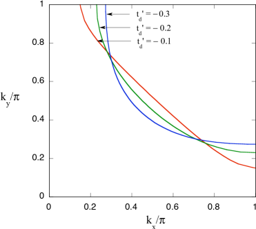
Figure 2: Fermi surface of the 2D d-p model for $t_{pp}=0.4$ and $\Delta_{dp}=2.0$ where $t_{d}^{\prime}=-0.1$, $t_{d}^{\prime}=-0.2$ and $t_{d}^{\prime}=-0.3$ in units of $t_{dp}$. The carrier density is $n_{h}\sim 0.1$.

Wave function of Mott state Here we propose a wave function to represent a Mott insulator. We first discuss it for the single-band Hubbard modelhub63 . The energy is measured in units of $t$ in this section. The charge-transfer Mott state of the three-band model will be given by a generalization of the one-band Mott state. The Gutzwiller function $\psi_{G}$ itself does not describe the insulating state because this function has no kinetic energy gain in the limit $g\rightarrow 0$. Wave functions for the Mott transition have been proposed for the single-band Hubbard model by considering the doublon-holon correlationyok04 ; yok06 or backflow correlationstoc11 . In the latter, a variational wave function with a Jastrow factor is considered. It seems, however, not straightforward to generalize these wave functions to the three-band case.

The Gutzwiller wave function is given as

$$\psi_{G}=P_{G}\psi_{0},$$ (3)

where $P_{G}$ is the Gutzwiller projection operator given by $P_{G}=\prod_{i}[1-(1-g)n_{i\uparrow}n_{i\downarrow}]$ with the variational parameter $g$ in the range from 0 to unity. $P_{G}$ controls the on-site electron correlation and $\psi_{0}$ is the Fermi sea in this paper. We consider the Gutzwiller function with an optimization operatoryan98 :

$$\psi_{\lambda}=\exp({\lambda K})\psi_{G},$$ (4)

where $K$ is the kinetic part of the Hamiltonian and $\lambda$ is a variational parameter. This type of wave function is an approximation to the wave function in quantum Monte Carlo methodhir81 ; yan07 ; yan13 . The operator $e^{\lambda K}$ lowers the energy considerably. We have finite energy gain with this function even in the limit $g\rightarrow 0$ due to the kinetic operator $K$. We show that $\psi_{\lambda}$ with vanishing $g$ describes a Mott insulator.

In Fig.3 we show the energy per site as a function of $U$ on a $10\times 10$ lattice with the periodic boundary conditions. The upper curve shows the energy for the Gutzwiller function and the lower one is for the optimized function $\psi_{\lambda}$. It is seen from Fig.3 that the ground-state energy changes the curvature near $U\sim U_{c}$. This suggests that there is a transition from a metal to an insulator. We show the parameter $g$ on $10\times 10$ lattice in Fig.4. The parameter $g$ vanishes at a critical value $U_{c}\sim 8$. The energy for $\psi_{\lambda}$ is well approximated by a function $C/U$ with a constant $C$ when $U$ is large:

$$\frac{E}{N}\sim-C\frac{t^{2}}{U}\propto-CJ.$$ (5)

This means that the energy gain mainly comes from the exchange interaction which is of the order of $1/U$, showing that the ground state is insulating. The effective interaction in the limit of large $U$ is given by the effective interaction, given by $J\sum_{\langle ij\rangle}{\bf S}_{i}\cdot{\bf S}_{j}$ with $J=4t^{2}/U$, and the three-site interactionshar67 if we consider only the nearest-neighbor transfer $t$. In our calculation, we have $C\sim 3$. This means that the ground-state energy per site is approximately given by $E/N\sim-0.75J$. This value, $-0.75J$, will become better by improving the wave function $\psi_{\lambda}$yan98 . The inset in Fig.4 exhibits that there is a singularity in $g$ at $U\simeq U_{c}$ as a function of $U$. There is a small jump in $g$. This indicates that the transition is first order.

The Fig.5 shows the momentum distribution function $n_{k}$:

$$n_{{\bf k}}=\frac{1}{2}\sum_{\sigma}\langle c_{{\bf k}\sigma}^{{\dagger}}c_{{\bf k}\sigma}\rangle.$$ (6)

There is clearly the gap in $n_{k}$ at the Fermi surface for small $U$, namely, $U\leq 6$. In contrast, for large $U$ being greater than 7, the gap at the Fermi surface disappears. This indicates that the ground state is an insulator for large $U$. This is consistent with the VMC study in Ref.yok06 where the different trial wave function is adopted. Other quantities are also consistent. The critical value of $U$ is consistent; both have given $U_{c}\sim 7t$. The ground-state energy is also well approximated by a curve $t^{2}/U$ when $U$ is large beyond the critical value.

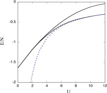
Figure 3: Ground state energy of the 2D Hubbard model per site as a function $U$ at half-filling on $10\times 10$ lattice. We set $t^{\prime}=-0.2$. The upper curve is for the Gutzwiller function and the lower curve is for $\psi_{\lambda}$. The dotted line shows a curve C/U where $C(<0)$ is a constant.

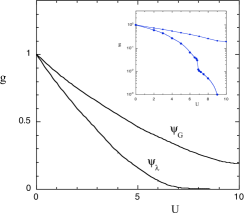
Figure 4: Gutzwiller parameter $g$ as a function of $U$ at half-filling on $10\times 10$ lattice with $t^{\prime}=-0.2$. The parameter $g$ almost vanishes at $U\sim 8$ as for $6\times 6$ lattice. The upper line is for the Gutzwiller function and the lower is for $\psi_{\lambda}$. The inset shows $g$ using a logarithmic scale.

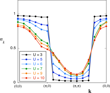
Figure 5: Momentum distribution function $n_{k}$ for $\psi_{\lambda}$ at half-filling on $10\times 10$ lattice. We show $n_{k}$ for $U=3,5,6,7,9$ and 10. $n_{k}$ shows the insulating behavior for $U\geq 7$.

Figure 6: Parameters $g$ and $\lambda$ as a function of $\Delta_{dp}$ at half-filling on $6\times 6$ lattice. We used $t_{pp}=0.4$, $t_{d}^{\prime}=-0.0$ and $U_{d}=8$ (in units of $t_{dp}$). The upper line is for the Gutzwiller function and the lower is for $\psi_{\lambda}$.

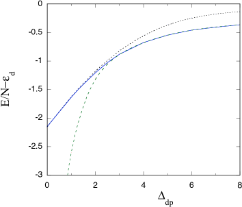
Figure 7: Ground state energy of the 2D d-p model as a function of $\Delta_{dp}$ for $t_{pp}=0.0$, $t_{d}^{\prime}=-0.0$ and $U_{d}=8$ (in units of $t_{dp}$) in the half-filled case. The calculations were performed on $6\times 6$ lattice. The dotted curve is for the Gutzwiller function, namely $\lambda=0$. The dashed curve indicates a curve given by a constant times $1/(\epsilon_{p}-\epsilon_{d})$.

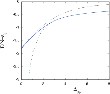
Figure 8: Ground state energy of the 2D d-p model as a function of $\Delta_{dp}$ for $t_{pp}=0.4$, $t_{d}^{\prime}=-0.2$ and $U_{d}=8$ (in units of $t_{dp}$) in the half-filled case. The calculations were performed on $6\times 6$ lattice. The dotted curve is for the Gutzwiller function with $\lambda=0$. The dashed curve indicates a curve given by a constant times $1/(\epsilon_{p}-\epsilon_{d})$.

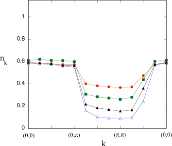
Figure 9: Momentum distribution function of d holes in the 2D d-p model for $t_{pp}=0.4$, $t_{d}^{\prime}=-0.0$ and $U_{d}=8$ (in units of $t_{dp}$) in the half-filled case on $8\times 8$ lattice. From the top, $\epsilon_{p}-\epsilon_{d}=6$, 4, 2 for $\psi_{\lambda}$ and the bottom is for the Gutzwiller function with $\epsilon_{p}-\epsilon_{d}=2$.

Charge-transfer Mott state In this section, we consider the ground state of the three-band d-p model in the half-filled case. The energy unit is given by $t_{dp}$ in this section. The Gutzwiller wave function for the d-p model is $\psi_{G}=P_{G}\psi_{0}$, where $P_{G}$ is the Gutzwiller projection operator for d electrons. We neglect the on-site Coulomb repulsion on the oxygen site because it is not important when the number of p holes is small. $\psi_{0}$ is a one-particle wave function given by the Fermi sea. $\psi_{0}$ contains the variational parameters $\tilde{t}_{dp}$, $\tilde{t}_{pp}$, $\tilde{t}_{d}^{\prime}$, $\tilde{\epsilon}_{d}$ and $\tilde{\epsilon}_{p}$:

$$\psi_{0}=\psi_{0}(\tilde{t}_{dp},\tilde{t}_{pp},\tilde{t}_{d}^{\prime},\tilde{\epsilon}_{d},\tilde{\epsilon}_{p}).$$ (7)

In the non-interacting case, $\tilde{t}_{dp}$, $\tilde{t}_{pp}$ and $\tilde{t}_{d}^{\prime}$ coincide with $t_{dp}$, $t_{pp}$ and $t_{d}^{\prime}$ in the Hamiltonian, respectively. As we have shown, $t_{d}^{\prime}$ plays an important role to determine the Fermi surface within the d-p model. The Fermi surface is determined by $\tilde{t}_{dp}$, $\tilde{t}_{pp}$ and $\tilde{t}_{d}^{\prime}$ in the correlated wave function.

The optimized wave function is

$$\psi_{\lambda}=\exp(\lambda K)\psi_{G},$$ (8)

where $K$ is the kinetic part of the total Hamiltonian $H_{dp}$ and $\lambda$ is a variational parameter. In general, the band parameters $t_{pp}$, $t^{\prime}_{d}$, $\epsilon_{d}$ and $\epsilon_{p}$ in $K$ are regarded as variational parameters:

$$K=K(\hat{t}_{pp},\hat{t^{\prime}_{d}},\hat{\epsilon_{d}},\hat{\epsilon_{p}}).$$ (9)

For simplicity, we take $\hat{t}_{pp}=\tilde{t}_{pp}$, $\hat{t^{\prime}}_{d}=\tilde{t^{\prime}}_{d}$, $\hat{\epsilon}_{d}=\tilde{\epsilon}_{d}$ and $\hat{\epsilon}_{p}=\tilde{\epsilon}_{p}$. The energy expectation value is minimized for variational parameters $g$, $\tilde{t}_{dp}$, $\tilde{t}_{pp}$, $\tilde{t}_{d}^{\prime}$, $\tilde{\epsilon}_{p}-\tilde{\epsilon}_{d}$ and $\lambda$.

We show the parameter $g$ as a function of $\Delta_{dp}$ for $U_{d}=8$, $t_{pp}=0.4$ and $t^{\prime}_{d}=0$ on $6\times 6$ lattice in Fig.6. $g$ of $\psi_{\lambda}$ is decreasing rapidly for positive $\Delta_{dp}$ and vanishes at $\Delta_{dp}\sim 0.5t_{dp}$ while that in $\psi_{G}$ decreases gradually as a function of $\Delta_{dp}$. The figure 8 exhibits the ground-state energy per site $\Delta E\equiv E/N-\epsilon_{d}$ as a function of $\Delta_{dp}$ for $t_{pp}=0$, $t_{d}^{\prime}=0$ and $U_{d}=8$. This set of parameters correspond to that for LSCO. We can find that the curvature of the energy, as a function of $\Delta_{dp}$, is changed near $\Delta_{dp}\sim 2t_{dp}$. This means that the region $\Delta_{dp}>2t_{dp}$ is a large-$\Delta_{dp}$ region. The energy is well fitted by $1/\Delta_{dp}$ shown by the dashed curve in Fig.7 when $\Delta_{dp}$ is greater than the critical value $(\Delta_{dp})_{c}\sim 2t_{dp}$. A similar behavior is also observed for the other set of parameters such as $t_{pp}=0.4$, $t_{d}^{\prime}=-0.2$ and $U_{d}=8$ for Bi2212, Tl2201 and Hg1201, as shown in Fig.8. We show the momentum distribution for d electrons defined by $n_{k}=\langle d_{k\sigma}^{{\dagger}}d_{k\sigma}\rangle$ in Fig.9. This was calculated on $8\times 8$ lattice and exhibits the effect of correlation in the localized region.

The results indicate that the energy gain $\Delta E$ mostly comes from the second-order perturbation with the excitation energy $\Delta_{dp}$. Thus, in general, the energy gain $\Delta E$ is expanded in terms of $\Delta_{dp}^{-1}$ when $\Delta_{dp}$ is large:

$$\Delta E\simeq\frac{A_{1}}{\Delta_{dp}}+\frac{A_{2}}{\Delta_{dp}^{2}}+\cdots.$$ (10)

As seen from Figs.7 and 8, $A_{1}$ is negative and $A_{2}$ is positive. It is known that the antiferromagnetic exchange interaction works between d electrons on neighboring copper atoms. The coupling $J_{Cu-Cu}$ is given asesk93 ; kam94

$$J_{Cu-Cu}=\frac{4t_{dp}^{2}}{(\Delta_{dp}+U_{dp})^{2}}\left(\frac{1}{U_{d}}+\frac{2}{2\Delta_{dp}+U_{p}}\right).$$ (11)

The exchange coupling $J_{Cu-Cu}$ will give the energy gain being proportional to $1/\Delta_{dp}^{2}$ when the d electrons are antiferromagnetically aligned on copper atoms. Our results show that this contribution is small keeping $A_{2}$ positive.

For large $\Delta_{dp}$ the energy gain is proportional to $1/\Delta_{dp}$:

$$\Delta E=\frac{E}{N}-\epsilon_{d}\simeq-C\frac{t_{dp}^{2}}{\Delta_{dp}},$$ (12)

for a constant $C$. This indicates that the ground state is an insulator of charge-transfer type. In our calculation we obtain $C\sim 3$.

Summary We have proposed a wave function of Mott insulator based on an optimized Gutzwiller function in strongly correlated electron systems. We have investigated Mott transition at half-filling in the single-band Hubbard model first and generalized it to the three-band d-p model by employing the variational Monte Carlo method. The metal-insulator transition occurs as a result of strong correlation. The wave function in this paper describes a first-order transition from a metal to a Mott insulator.

Our wave function has the form

$$\psi_{\lambda}=e^{\lambda K}\psi_{G}(g),$$ (13)

where $g$ is the Gutzwiller parameter. The limit $g\rightarrow 0$ indicates no double occupancy of d holes in $\psi_{G}$. In this limit the energy of the single-band Hubbard model is given by that of the strong-coupling limit $U\gg t$, namely, $E\propto-t^{2}/U$. This means that $\psi_{\lambda}$ is an insulator in the limit $g\rightarrow 0$. This state indeed becomes stable when $U$ is as large as $7t$. This shows that there is a metal-insulator transition at $U=U_{c}\sim 7t$. There is a singularity in $g$ at $U\simeq U_{c}$ as a function of $U$, indicating that the transition is first order. The same discussion also holds for the three-band d-p model except that the cuprates exhibit charge-transfer transition. In the localized region with large $\Delta_{dp}$, the energy of $\psi_{\lambda}$ with vanishing $g$ is given by $E/N-\epsilon_{d}\sim-t_{dp}^{2}/\Delta_{dp}$, indicating that $\psi_{\lambda}$ is a charge-transfer insulator. The stabilization of $\psi_{\lambda}$ for large $U_{d}$ and $\Delta_{dp}$ shows the existence of a metal-insulator transition in the d-p model. The transition occurs for the band parameters that are suitable for high temperature cuprates. Our result shows that $(\Delta_{dp})_{c}\sim 2t_{dp}$. If we use $t_{dp}\simeq 1.5$eVhyb89 ; esk89 ; mcm90 , the charge-transfer insulator has a gap of 3eV.

Finally, we give a discussion on magnetism. The competition between magnetic state and paramagnetic state would depend on band parameters. There would be a transition from a magnetic insulator to a paramagnetic insulator as the band parameters are varied. We expect that $t_{d}^{\prime}$ plays an important role in this transition because $t_{d}^{\prime}$ would play a similar role to the next-nearest neighbor transfer integral $t^{\prime}$ in the single-band Hubbard model.

We express sincere thanks to J. Kondo, K. Yamaji and I. Hase for useful discussions. This work was supported by a Grant-in-Aid for Scientific Research from the Ministry of Education, Culture, Sports, Science and Technology of Japan. A part of the numerical calculations was performed at the Supercomputer Center of the Institute for Solid State Physics, University of Tokyo.

References

- (1) The Physics of Superconductor (Vol.I and Vol.II) edited by K. H. Bennemann and J. B. Ketterson (Springer-Verlag, Berlin, 2003).
- (2) J. Zaanen, G. A. Sawatzky and J. W. Allen, Phys. Rev. Lett. 55, 418 (1985).
- (3) J. E. Hirsch, E. Y. Loh, D. J. Scalapino and S. Tang: Phys. Rev. B39, 243 (1989).
- (4) R. T. Scalettar, D. J. Scalapino, R. L. Sugar, and S. R. White: Phys. Rev. B44, 770 (1991).
- (5) M. Guerrero, J. E. Gubernatis and S. Zhang: Phys. Rev. B57, 11980 (1998).
- (6) S. Koikegami and K. Yamada: J. Phys. Soc. Jpn. 69, 768 (2000).
- (7) T. Yanagisawa, S. Koike and K. Yamaji: Phys. Rev. B64, 184509 (2001); ibid. B67, 132408 (2003).
- (8) T. Yanagisawa: New J. Physics 10, 023014 (2008).
- (9) T. Yanagisawa, M. Miyazaki and K. Yamaji: J. Phys. Soc. Jpn. 78, 013706 (2009).
- (10) C. Weber, A. Lauchi, F. Mila and T. Giamarchi: Phys. Rev. Lett. 102, 017005 (2009).
- (11) B. Lau, M. Berciu and G. A. Sawatzky: Phys. Rev. Lett. 106, 036401 (2011).
- (12) T. Yanagisawa, M. Miyazaki and K. Yamaji: J. Mod. Phys. 4, 33 (2013).
- (13) C. Gros, R. Joynt, and T. M. Rice: Phys. Rev. B36, 381 (1987).
- (14) H. Yokoyama and H. Shiba: J. Phys. Soc. Jpn. 56, 1490 (1987).
- (15) T. Nakanishi, K. Yamaji and T. Yanagisawa: J. Phys. Soc. Jpn. 66, 294 (1997).
- (16) K. Yamaji, T. Yanagisawa, T. Nakanishi and S. Koike: Physica C 304, 225 (1998).
- (17) K. Yamaji, T. Yanagisawa and S. Koike: Physica B284-288, 415 (2000).
- (18) M. Miyazaki, T. Yanagisawa and K. Yamaji: J. Phys, Soc. Jpn. 73, 1643 (2004); ibid. 78, 043706 (2009).
- (19) C. Weber, K. Haule and G. Kotliar: Phys. Rev. B78, 134519 (2008).
- (20) M. S. Hybertsen, M. Schluter and N. E. Christensen: Phys. Rev. B39, 9028 (1989).
- (21) H. Eskes, G. A. Sawatzky and L. F. Feiner: Physica C160, 424 (1989).
- (22) A. K. McMahan, J. F. Annett and R. M. Martin: Phys. Rev. B42, 6268 (1990).
- (23) H. Eskes and G. Sawatzky: Phys. Rev. B43, 119 (1991).
- (24) J. Hubbard: Proc. Roy. Soc. A276, 237 (1963).
- (25) T. Yanagisawa, M. Miyazaki and K. Yamaji: JPS Conf. Proc. 3, 015046 (2014).
- (26) O. K. Andersen, A. I. Liechtenstein, O. Jepsen and F. Paulsen: J. Phys. Chem. Solids 56, 1573 (1995).
- (27) K. McElroy, R. W. Simmonds, J. E. Hoffman, D.-H. Lee, J. Orenstein, H. Eisaki, S. Uchida and J. C. Davis: Nature 422, 592 (2003).
- (28) N. E. Hussey, M. Abdel-Jawad, A. Carrington, A. P. Mackenzie and L. Balicas: Nature 425, 814 (2003).
- (29) D. J. Singh and W. E. Pickett: Physica C203, 193 (1992).
- (30) M. Plate, D. F. Mottershead, I. B. Elfimov, D. C. Peets, R. Liang, D. A. Bonn, W. H. Hardy, S. Chluzbalan, M. Falub, M. Shi, L. Patthey and A. Damascelli: Phys. Rev. Lett. 95, 07001 (2005).
- (31) W. S. Lee et al.: arXiv cond-mat/0606347 (2006).
- (32) H. Yokoyama, Y. Tanaka, M. Ogata and H. Tsuchiura: J. Phys. Soc. Jpn. 73, 1119 (2004).
- (33) H. Yokoyama, M. Ogata and Y. Tanaka: J. Phys. Soc. Jpn. 75, 114706 (2006).
- (34) L. F. Tocchio, F. Becca and C. Gross: Phys. Rev. B83, 195138 (2011).
- (35) T. Yanagisawa, S. Koike and K. Yamaji: J. Phys. Soc. Jpn. 67, 3867 (1998); ibid. 68, 3608 (1999).
- (36) J. E. Hirsch, D. J. Scalapino and R. L. Sugar: Phys. Rev. Lett. 47, 1628 (1981).
- (37) T. Yanagisawa: Phys. Rev. B75, 224503 (2007).
- (38) T. Yanagisawa: New J. Phys. 15, 033012 (2013).
- (39) A. B. Harris and R. V. Range: Phys. Rev. 157, 295 (1967).
- (40) H. Eskes and J. H. Jefferson: Phys. Rev. B48, 9788 (1993).
- (41) A. P. Kampf: Phys. Rep. 249, 219 (1994).