Preconditioned Locally Harmonic Residual Method for Computing Interior Eigenpairs of Certain Classes of Hermitian Matrices

Abstract

We propose a Preconditioned Locally Harmonic Residual (PLHR) method for computing several interior eigenpairs of a generalized Hermitian eigenvalue problem, without traditional spectral transformations, matrix factorizations, or inversions. PLHR is based on a short-term recurrence, easily extended to a block form, computing eigenpairs simultaneously. PLHR can take advantage of Hermitian positive definite preconditioning, e.g., based on an approximate inverse of an absolute value of a shifted matrix, introduced in [SISC, 35 (2013), pp. A696–A718]. Our numerical experiments demonstrate that PLHR is efficient and robust for certain classes of large-scale interior eigenvalue problems, involving Laplacian and Hamiltonian operators, especially if memory requirements are tight.

1 Introduction

We are interested in computing a subset of eigenpairs of the generalized Hermitian eigenvalue problem

(1) $$Av=\lambda Bv,\quad A=A^{*}\in\mathbb{C}^{n\times n},\quad B=B^{*}>0\in\mathbb{C}^{n\times n},$$

that correspond to eigenvalues closest to a given shift $\sigma$, which is real and points to the eigenvalues in the interior of the spectrum. We refer to (1) as an interior eigenproblem, and call the targeted eigenpairs interior eigenpairs.

Interior eigenpairs are of fundamental interest in some physical models, e.g., for first-principles electronic structure analysis of materials using a semi-empirical potential or a charge patching method [37, 38, 39]. There, the requested eigenvalues correspond to energy levels around a material-dependent energy shift $\sigma$, and the eigenvectors represent the associated wave functions.

We assume that the size $n$ of the matrices is so large that eigenvalue solvers based on explicit matrix transformations are impractical. Other conventional ways of solving the interior eigenvalue problems are based on spectral transformations that allow reducing the interior eigenproblem to an easier task of computing extreme (smallest or largest) eigenvalues of a transformed pencil. Such transformations include the so-called shift-and-invert (SI) and folded spectrum (FS) approaches; see, e.g., [2]. While both techniques are extensively used, they face serious issues as $n$ increases.

In particular, SI relies on repeated solution of large shifted linear systems, which generally becomes extremely inefficient or infeasible for large $n$. Similar difficulties are experienced in methods relying on contour integration, e.g., [29].

The FS approach for standard, i.e., with identity $B=I$, eigenproblems is inverse-free. However, in exact arithmetic, it is equivalent to solving an eigenproblem for the matrix $(A-\sigma I)^{2}$, which squares the condition number, resulting in severely tightened clustering of the targeted eigenvalues. For the generalized, i.e., with $B\neq I$, eigenproblems, FS requires inverting the matrix $B$, which can be problematic. Additionally, available preconditioning, normally based on approximating an inverse of $A-\sigma B$, may not be applicable for FS, which should be preconditioned by an approximate inverse of the squared operator.

For certain classes of eigenproblems, multigrid (MG) algorithms have proved to be very efficient; see, e.g., [3, 10, 19, 20] and references therein. However, the applicability of such eigensolvers faces the same kind of limitations as exist for the MG linear solvers in that either geometric (grid) information must be available at solution time or the problem’s structure should be appropriate for the algebraic MG approaches.

Another popular technique for interior eigenproblems is based on combining polynomial transformations, called filters, with the standard Lanczos method, as in filtered Lanczos procedure [6]. The approach cannot easily be extended to generalized eigenproblems and does not take advantage of preconditioners that may be available.

Residual minimization scheme, direct inversion in the iterative subspace (RMM-DIIS), see [40], provides an alternative, but is known to be unreliable if the initial approximations are not close enough to the targeted eigenpairs. RMM-DIIS has to be preceded by, e.g.,  generalized Davidson [22] or Jacobi–Davidson [30] methods, such as, e.g., in Vienna ab initio simulations (VASP) package [18]. Combining harmonic Rayleigh–Ritz (RR) procedure  [2] with the Davidson’s family of methods has recently aimed at supplementing RMM-DIIS in VASP; see [12].

Success of the Davidson type methods is often determined by two interdependent algorithmic components: the maximum allowed size of the search subspace and the quality of the preconditioner, typically given as a form of an approximate solve of the system with a shifted matrix $A-\sigma B$. The maximum size of the search subspace has to be increased if the preconditioner quality deteriorates. In practical computations, preconditioners that lack the desired quality are common, especially if the shift $\sigma$ targets the eigenvalues that are deep in the interior of the spectrum.

We develop new preconditioned iterative schemes for interior eigenproblems that exhibit a lower sensitivity to the preconditioner quality and at the same time lead to fixed and relatively modest memory requirements. A connection between iterative methods for singular homogeneous Hermitian indefinite systems and eigenproblems in Section 2 motivates our development. Our base method, called Preconditioned Locally Harmonic Residual (PLHR) and presented in Section 3, computes a single eigenpair. In Section 4, we generalize PLHR to block iterations, where targeted eigenpairs, as determined by $\sigma$, are computed simultaneously, similar to LOBPCG [15].

PLHR requires that the preconditioner is Hermitian positive definite (HPD). In Section 5, we suggest that the preconditioner $T$ should approximate the inverted matrix absolute value $|A-\sigma B|$. Preconditioners of this kind, called the absolute value (AV) preconditioners, have been recently introduced in [35]. In particular, [35] describes an MG scheme for approximating the inverse of the AV of the shifted Laplacian. Thus, the approach can be directly applied as a PLHR preconditioner for computing interior eigenpairs of the Laplacian matrix, which is demonstrated in our numerical experiments in Section 6. Furthermore, the suitable HPD preconditioners are readily available in electronic structure calculations, where we combine PLHR with the existing state-of-the-art preconditioner [32], also in Section 6.

While, in this work, we focus only on several model problems with already available HPD preconditioners, the proposed PLHR approach can be applicable to broader classes of eigenproblems that admit appropriate HPD preconditioning. Investigation of such problems, as well as the development of the corresponding preconditioners, is a matter of future research, and is outside the scope of the current paper.

An important novelty of the proposed approach is a modification of the harmonic RR procedure, obtained by a proper utilization of the HPD preconditioner $T$ in the Petrov-Galerkin condition for extracting the approximate eigenvectors, including its real arithmetic implementation. The new extraction technique, that we call the $T$-harmonic RR procedure in Section 3, is critical. Our tests demonstrate remarkable robustness if the $T$-harmonic procedure is used. The gains are especially evident if the preconditioner quality deteriorates, whereas the memory requirements remain fixed.

2 Preconditioned null space computations

We start with an easier problem of finding a null space component of a Hermitian matrix. Let $\lambda_{q}$ be a targeted eigenvalue of (1) closest to the shift $\sigma$. We assume that $\lambda_{q}$ is known. Then eigenproblem (1) turns into the singular homogeneous linear system

(2) $$(A-\lambda_{q}B)v=0.$$

It is clear that (2) has a non-trivial null space solution determining an eigenvector $v_{q}$ associated with $\lambda_{q}$. Thus, in the idealized setting, where $\lambda_{q}$ is available, an eigensolver for (1) can be given by an appropriate solution scheme for linear system (2). In this sense, linear solvers for (2) can be viewed as prototypical, or idealized, methods for computing the eigenpair $(\lambda_{q},v_{q})$.

The described connection between linear and eigenvalue solvers has been emphasized in literature; see, e.g.,  [13, 15]. For example, in [15], a special case is considered where $\lambda_{q}$ is the smallest eigenvalue of (1) and, hence, the system (2) is Hermitian positive semidefinite. A proper choice of the linear solver—a three-term recurrent form of the preconditioned conjugate gradient (PCG) method—has led to derivation of the popular LOBPCG algorithm for finding extreme eigenpairs; see [15, 16].

We follow a similar approach. Assuming that $\lambda_{q}$ is known, we select efficient preconditioned linear solvers capable of computing a non-trivial solution of (2). Viewing these linear solvers as idealized eigensolvers, we then extend them to the practical case where $\lambda_{q}$ is unknown.

Since the targeted eigenvalue $\lambda_{q}$ can be located anywhere in the interior of the spectrum of the pencil $A-\lambda B$, the Hermitian coefficient matrix of system (2) is generally indefinite in contrast to [15], which makes PCG inapplicable. We look for suitable preconditioned short-term recurrent Krylov subspace type methods that can be applied to singular Hermitian indefinite systems of the form (2) and guarantee linear convergence.

An optimal technique in this class of methods is the preconditioned minimal residual (PMINRES) algorithm [25]. While most commonly applied to non-singular systems, the method is also guaranteed to work for a class of singular consistent Hermitian systems, such as (2). The preconditioner for PMINRES should normally be HPD, and the convergence of the method is governed by the spectrum distribution of the preconditioned matrix. However, the standard implementation of the algorithm is deeply rooted in the Lanczos procedure, where the availability of the matrix $A-\lambda_{q}B$ is crucial at every stage of the process. Since this assumption is not realistic in the context of eigenvalue computations, where only an approximation of $\lambda_{q}$ is at hand, PMINRES fails to provide a proper insight into the structure of local subspaces that determine a new approximate solution. Similar arguments apply to methods that are mathematically equivalent to PMINRES, such as, e.g., orthodir($3$) [9, 27, 42].

Returning back for a moment to the special case where $\lambda_{q}$ is the smallest eigenvalue of (1), a preconditioned steepest descent (PSD) linear solver can be viewed as a predecessor of the PCG linear solver, on the one hand, and as restarted preconditioned Lanczos linear solver, on the other hand. We use this viewpoint to describe an analog of a PSD-like linear solver for the indefinite case.

To that end, we restart PMINRES in such a way that linear convergence is preserved (possibly with a lower rate), whereas the number of steps between the restarts is kept to a minimum possible. It is shown in [34] that in order to maintain PMINRES convergence, the number of steps between the restarts should be no smaller than two. Thus, the simplest convergent residual minimizing iteration for (2) is

(3) $$v^{(i+1)}=v^{(i)}+\alpha^{(i)}Tr^{(i)}+\beta^{(i)}T\left(A-\lambda_{q}B\right)Tr^{(i)},\quad i=0,1,\ldots;\\$$

where $r^{(i)}=\left(\lambda_{q}B-A\right)v^{(i)}$ and the iteration parameters $\alpha^{(i)}$, $\beta^{(i)}$ are chosen to minimize the $T$-norm of the residual $r^{(i+1)}$, i.e., are such that

(4) $$\|r^{(i+1)}\|_{T}=\min_{u\in\mathcal{K}^{(i)}}\|r^{(i)}-(A-\lambda_{q}B)u\|_{T},$$

where

(5) $$\mathcal{K}^{(i)}=\text{span}\left\{Tr^{(i)},T(A-\lambda_{q}B)Tr^{(i)}\right\}.$$

Here and throughout, for a given HPD matrix $M$, the corresponding vector $M$-norm is defined as $\|\cdot\|_{M}=(\cdot,M\cdot)^{1/2}$.

Theorem 1 ([34]).

Given an HPD preconditioner $T$, the iteration (3)–(5) converges to a nontrivial solution of (2), provided that the initial guess $x^{(0)}$ has a non-zero projection onto the null space of $A-\lambda_{q}B$. Moreover, if $\lambda_{q}$ is a simple eigenvalue of $A-\lambda B$ and $\mu_{1}\leq\mu_{2}\leq\ldots\leq\mu_{q-1}<\mu_{q}=0<\mu_{q+1}<\ldots\mu_{n}$ are the eigenvalues of the preconditioned matrix $T(A-\lambda_{q}B)$, then the residual norm reduction is given by

(6) $$\frac{\|r^{(i+1)}\|_{T}}{\|r^{(i)}\|_{T}}\leq\frac{\tilde{\kappa}-1}{\tilde{\kappa}+1}<1,$$

where

(7) $$\tilde{\kappa}=\left\{\begin{array}[]{l}\displaystyle\left(\frac{\mu_{n}}{\mu_{q+1}}\right)\left(1+\frac{\mu_{n}-\mu_{q+1}}{\left|\mu_{q-1}\right|}\right),\ \mbox{if}\ \left|\mu_{1}\right|-\left|\mu_{q-1}\right|\leq\mu_{n}-\mu_{q+1}\\ \\ \displaystyle\left(\frac{\mu_{1}}{\mu_{q-1}}\right)\left(1+\frac{\left|\mu_{1}\right|-\left|\mu_{q-1}\right|}{\mu_{q+1}}\right),\ \mbox{if}\ \left|\mu_{1}\right|-\left|\mu_{q-1}\right|>\mu_{n}-\mu_{q+1}.\end{array}\right.$$

The proof of Theorem 1 relies on the analysis of iterations of the form (3), where the parameters $\alpha^{(i)}$ and $\beta^{(i)}$ are fixed. In this case, (3) can be viewed as a stationary Richardson type scheme for a polynomially preconditioned system, and a standard convergence analysis (see, e.g., [1, Theorem 5.6]) applies to determine the values of the parameters that yield an optimal convergence, which is given by (6)–(7). Since the convergence of the stationary iteration cannot be better then that of (3) with the residual minimizing parameters (4), bound (6)–(7) immediately applies to method (3)–(5). For more details, we refer the reader to [34].

A natural way to enhance (3)–(5) is by introducing an additional term that holds information from the previous step. By analogy with a three-term recurrent form of PCG, consider the scheme

(8) $$v^{(i+1)}=v^{(i)}+\alpha^{(i)}Tr^{(i)}+\beta^{(i)}T\left(A-\lambda_{q}B\right)Tr^{(i)}+\gamma^{(i)}(v^{(i)}-v^{(i-1)}),\ i=0,1,\ldots,\\$$

where $v^{(-1)}=0$. Here, the scalar parameters $\alpha^{(i)}$, $\beta^{(i)}$, and $\gamma^{(i)}$ are chosen according to local minimality condition (4) with

(9) $$\mathcal{K}^{(i)}=\text{span}\left\{Tr^{(i)},T(A-\lambda_{q}B)Tr^{(i)},v^{(i)}-v^{(i-1)}\right\}.$$

Since $\mathcal{K}^{(i)}$ in (9) contains the subspace in (5), the employed minimality condition (4) implies that convergence of (8) is not worse than that of (3). Hence, the results of Theorem 1 also apply to (8) with (4) and (9). In this case, however, bound (6)–(7) is likely to be an overestimate, and in practice the presence of the additional vector in the recurrence leads to a faster convergence. In fact, the scheme (8) has been observed to exhibit behavior similar to PMINRES up to the occurrence of superlinear convergence [34], which is a consequence of the global optimality of the latter. Additionally, iteration (8) reveals the structure of local subspaces that are used to determine the improved approximate solution, which we exploit in the next section for constructing the trial subspaces in the context of the eigenvalue calculations.

For these reasons, we choose (8) with (4) and (9) to be a “base” linear solver for the null space problem (2) and, in what follows, use it as a starting point for deriving preconditioned interior eigensolvers.

3 The Preconditioned Locally Harmonic Residual method

We now present an approach for computing an eigenpair $(\lambda_{q},v_{q})$ of (1) that corresponds to the eigenvalue closest to a given shift $\sigma$. The method is motivated by the preconditioned null space finders discussed in the previous section. Our idea is to extend the “base” linear solver (8) to the case of eigenvalue computations by introducing a series of approximations into recurrence (8) and optimality condition (4).

The null space finding scheme (8) suggests that, if $\lambda_{q}$ is known, the improved eigenvector approximation $v^{(i+1)}$ belongs to the subspace

(10) $$\mbox{span}\left\{v^{(i)},T(A-\lambda_{q}B)v^{(i)},T(A-\lambda_{q}B)T(A-\lambda_{q}B)v^{(i)},v^{(i-1)}\right\}.$$

Clearly, in practice, the exact value of $\lambda_{q}$ is unavailable and, hence, the computation of (10) cannot be performed. In order to obtain a computable subspace in the context of eigenvalue problem (1), we approximate $\lambda_{q}$ by the Rayleigh Quotient (RQ)

$$\lambda^{(i)}\equiv\lambda(v^{(i)})=(v^{(i)},Av^{(i)})/(v^{(i)},Bv^{(i)}).$$

As a result, at each iteration $i$, the following trial subspace is introduced:

(11) $$\mathcal{Z}^{(i)}=\mbox{span}\left\{v^{(i)},w^{(i)},s^{(i)},v^{(i-1)}\right\},$$

where $w^{(i)}=T(Av^{(i)}-\lambda^{(i)}v^{(i)})$ is the preconditioned residual for problem (1), and $s^{(i)}=T(Aw^{(i)}-\lambda^{(i)}w^{(i)})$.

Next, we address the question of extracting an approximate eigenpair from the subspace $\mathcal{Z}^{(i)}$. Let us recall that minimality principle (4), utilized by the base null space finder, implies the orthogonality relation

(12) $$r^{(i+1)}\equiv(A-\lambda_{q}B)v^{(i+1)}\perp_{T}(A-\lambda_{q}B)\mathcal{K}^{(i)},$$

where “$\perp_{T}$” denotes the “orthogonality in the $T$-based inner product” and $\mathcal{K}^{(i)}$ is defined in (9). Following the analogy with the linear solver, in the context of the eigenvalue problem, we introduce a similar condition:

(13) $$(A-\theta B)v^{(i+1)}\perp_{T}(A-\sigma B)\mathcal{Z}^{(i)},\quad\|v^{(i+1)}\|_{B}=1.$$

Here, we find a $B$-unit vector $v^{(i+1)}$ and a scalar $\theta\in\mathbb{C}$ that ensure the orthogonality of the vector $(A-\theta B)v^{(i+1)}$ to the subspace $(A-\sigma B)\mathcal{Z}^{(i)}$.

Condition (13) has been obtained from (12) as a result of two modifications. First, the known eigenvalue $\lambda_{q}$ in the residual $r^{(i+1)}$ of linear system (2) has been replaced by an unknown $\theta$, giving rise to the residual like vector $(A-\theta B)v^{(i+1)}$ for the eigenvalue problem. Note that this vector should be distinguished from the standard eigenresidual $(A-\lambda^{(i+1)}B)v^{(i+1)}$, where $\lambda^{(i+1)}$ is the RQ. Since the orthogonality of $(A-\theta B)v^{(i+1)}$ in (13) is invariant with respect to the norm of $v^{(i+1)}$, for definiteness, we request that the vector has a unit $B$-norm.

The second modification has been the replacement of the subspace $(A-\lambda_{q}B)\mathcal{K}^{(i)}$ in the right-hand side of (12) by $(A-\sigma B)\mathcal{Z}^{(i)}$, where $\mathcal{Z}^{(i)}$ is the trial subspace defined in (11). We expect that $(A-\sigma B)\mathcal{Z}^{(i)}$ captures well the ideal subspace $(A-\lambda_{q}B)\mathcal{K}^{(i)}$. Note that in the case where $\lambda_{q}$ is known, $\mathcal{K}^{(i)}\subset\mathcal{Z}^{(i)}$. Hence, if $\sigma$ is close to the targeted eigenvalue, both subspaces are close to each other.

We next discuss a procedure for computing the pair $(\theta,v^{(i+1)})$ in  (13).

3.1 The $T$-harmonic Rayleigh–Ritz procedure

Motivated by (13), let us consider a general problem, where we are interested in finding a number of pairs $(\theta,v)$ that approximate eigenpairs of (1) corresponding to the eigenvalues closest a given shift $\sigma$, such that each $v$ belongs to a given $m$-dimensional subspace $\mathcal{Z}$, and

(14) $$(A-\theta B)v\perp_{T}(A-\sigma B)\mathcal{Z},\quad\|v\|_{B}=1.$$

One can immediately recognize that (14) represents the Petrov-Galerkin condition [2, 28] formulated with respect to the $T$-based inner product. In the standard case with $T=I$, this condition leads to the well known harmonic Rayleigh-Ritz (RR) procedure, where approximate eigenpairs are delivered by the harmonic Ritz pairs [22, 23, 24]. The corresponding vectors $Av-\theta Bv$ are sometimes called the harmonic residuals; see, e.g., [36].

Let a basis of $\mathcal{Z}$ be given by columns of an $n$-by-$m$ matrix $Z$, so that any element of the subspace can be expressed in the form $v=Zy$, where $y$ is a vector of coefficients. Then the orthogonality constraint (14) translates into

$$Z^{*}(A-\sigma B)T(A-\theta B)Zy=\textbf{0},\quad\|Zy\|_{B}=1.$$

This is equivalent to the eigenvalue problem

(15) $$Z^{*}(A-\sigma B)T(A-\sigma B)Zy=\xi Z^{*}(A-\sigma B)TBZy,\quad\|Zy\|_{B}=1,$$

where $\xi\equiv\theta-\sigma$.

It is clear that the smallest in the absolute value eigenvalues $\xi$ correspond to the values of $\theta$ closest to the shift $\sigma$. Thus, if $(\xi,y)$ are the eigenpairs of (15) associated with the eigenvalues of the smallest absolute value, then the candidate approximations to the desired eigenpairs of the original problem (1) can be chosen as $(\theta,Zy)$.

Definition 2.

Let $(\xi,y)$ be an eigenpair of (15). We call $(\theta,Zy)$ a $T$-harmonic Ritz pair, where $\theta=\xi+\sigma$ and $v=Zy$ are a $T$-harmonic Ritz value and vector, respectively. The corresponding vector $Av-\theta Bv$ is then referred to as the $T$-harmonic residual with respect to the subspace $\mathcal{Z}$ (or, simply, the $T$-harmonic residual).

In order to see why $T$-harmonic Ritz pairs can be expected to deliver reasonable approximations to the interior eigenpairs, let us introduce the substitution $Q=T^{\frac{1}{2}}(A-\sigma B)Z$ and rewrite (15) as

(16) $$Q^{*}(T^{\frac{1}{2}}B)(A-\sigma B)^{-1}B(T^{\frac{1}{2}}B)^{-1}Qy=\tau Q^{*}Qy,\quad\tau=\frac{1}{\xi}\equiv\frac{1}{\theta-\sigma}.$$

We note that (16) is the projected problem in the RR procedure for the matrix $H=(T^{\frac{1}{2}}B)(A-\sigma B)^{-1}B(T^{\frac{1}{2}}B)^{-1}$ with respect to the subspace spanned by the columns of $Q$. The solution of this problem yields the Ritz pairs $(\tau,Qy)$ that tend to approximate well the exterior eigenpairs of $H$; see, e.g., [26, 28, 31].

Since the matrix $H$ is similar through $T^{\frac{1}{2}}B$ to the “shift-and-invert” operator $(A-\sigma B)^{-1}B$, each of its eigenpairs is of the form $(1/(\lambda-\sigma),T^{\frac{1}{2}}Bv)$, where $(\lambda,v)$ is an eigenpair of (1). Thus, the desired interior eigenvalues of (1) near the target $\sigma$ correspond to the exterior (largest in the absolute value) eigenvalues of $H$, which can be well approximated by the Ritz values of (16). The associated Ritz vectors $Qy$ then represent approximations to the eigenvectors $T^{\frac{1}{2}}Bv$ of $H$, i.e., $T^{\frac{1}{2}}(A-\sigma B)Zy\equiv Qy\approx T^{\frac{1}{2}}Bv$. This implies that $Zy\approx\alpha v$ for some scalar $\alpha$.

3.2 The PLHR algorithm

We now summarize the developments of the preceding sections and introduce an iterative scheme that at each step constructs a low-dimensional trial subspace (11) and uses the $T$-harmonic RR procedure to extract an approximate eigenvector from this subspace. The extraction is based on solving a 4-by-4 (3-by-3, at the initial step) eigenvalue problem (15), which defines an appropriate $T$-harmonic Ritz pair. The $T$-harmonic Ritz vector is then used as a new eigenvector approximation. We call this scheme the Preconditioned Locally Harmonic Residual (PLHR) algorithm; see Algorithm 1 below.

Input: The matrices $A=A^{*}$ and $B=B^{*}>0$, a preconditioner $T=T^{*}>0$, the shift $\sigma$, and the initial guess $v^{(0)}$ for the eigenvector; Output: An eigenvalue $\lambda$ closest to $\sigma$ and the associated eigenvector $v$, $\|v\|_{B}=1$; 1:  $v\leftarrow v^{(0)}$; $v\leftarrow v/\|v\|_{B}$; $\lambda\leftarrow(v,Av)$; $p\leftarrow[\ ]$; 2:  while convergence not reached do 3:     Compute the preconditioned residual $w\leftarrow T(Av-\lambda Bv)$; 4:     Compute $s\leftarrow T(Aw-\lambda Bw)$; 5:     Find the eigenpair $(\xi,y)$ of (15), where $Z=\left[v,w,s,p\right]$, such that $|\xi|$ is the smallest; $y=(\alpha,\beta,\gamma,\delta)^{T}$ (at the initial step, $y=(\alpha,\beta,\gamma)^{T}$ and $\delta=0$); 6:     $p\leftarrow\beta w+\gamma s+\delta p$; 7:     $v\leftarrow\alpha v+p$; 8:     $v\leftarrow v/\|v\|_{B}$; $\lambda\leftarrow(v,Av)$; 9:  end while 10:  Return $(\lambda,v)$.

Algorithm 1 Preconditioned Locally Harmonic Residual (PLHR) algorithm

The initial guess $v^{(0)}$ in Algorithm 1 can be chosen as a random vector. In practical applications, however, certain information about the solution is available, and $v^{(0)}$ can give a reasonable approximation to the eigenvector of interest. Utilizing such initial guesses typically leads to a substantial decrease in the iteration count and is therefore advisable.

Note that each PLHR iteration constructs a residual of the eigenvalue problem that can be used to determine the convergence in step 2 of Algorithm 1. In some applications, appropriate stopping criteria rely on tracking the difference between eigenvalue approximations, evaluated in step 8, at the subsequent iterations.

An important property of Algorithm 1 is that, in contrast to the original problem (1), the $T$-harmonic problem (15) is no longer Hermitian. As such, (15) can have complex eigenpairs, i.e., the iteration parameters $y=(\alpha,\beta,\gamma,\delta)^{T}$ can be complex. Thus, the PLHR algorithm should be implemented using complex arithmetic, even if $A$ and $B$ are real. This feature is undesirable, e.g., because of the need to double the required storage to accommodate complex numbers. A real arithmetic version of the method for the real case is presented in Section 4.1.

In Algorithm 1, we follow the common practice of discarding the harmonic Ritz values and replacing them with the RQs associated with the newly computed Ritz vectors; see, e.g., [22, 23] for the standard harmonic case. In particular, we skip the $\theta(\equiv\xi+\sigma)$ values (determined in step 5 of Algorithm 1) and replace them with $\lambda(v)=(v^{*}Av)/(v^{*}Bv)$, where $v=Zy$ is the $T$-harmonic Ritz vector.

Note that, at each iteration $i$, Algorithm 1 (step 6) constructs a conjugate direction that can be expressed, in the superscripted notation, as

$$p^{(i+1)}=v^{(i+1)}-\alpha^{(i)}v^{(i)}\equiv\beta^{(i)}w^{(i)}+\gamma^{(i)}s^{(i)}+\delta^{(i)}p^{(i)},$$

and the method extracts an approximate eigenvector from the subspace spanned by $v^{(i)}$, $w^{(i)}$, $s^{(i)}$, and $p^{(i)}$. In exact arithmetic, this subspace is the same as $\mathcal{Z}^{(i)}$ defined in (11). The above formula is known to yield an improved numerical stability in calculating the trial subspaces in the LOBPCG algorithm [15]. We expect that a similar property will hold for PLHR, and therefore follow the same style for computing the conjugate directions in Algorithm 1.

If it is possible to store additional vectors that contain results of the matrix-vector multiplications with $A$, $B$, and $T(A-\sigma B)$, then Algorithm 1 can be implemented with two matrix-vector multiplications involving $A$ and $B$, and four applications of the preconditioner $T$. Two of the preconditioning operations result from the construction of the trial subspace in steps 3 and 4, whereas the other two are the consequence of the $T$-harmonic extraction.

3.3 Possible variations

The choice of the trial subspaces and of the extraction procedure, motivated by the preconditioned null space finding framework in Section 2, is not unique. For example, one can define the “s-vector” as $s^{(i)}=T(Aw^{(i)}-\theta^{(i)}Bw^{(i)})$, where instead of the RQ $\lambda^{(i)}$ the current $T$-harmonic value $\theta^{(i)}$ is used. Alternatively, it is possible to set $s^{(i)}=T(Aw^{(i)}-\sigma Bw^{(i)})$, i.e., use the fixed $\sigma$ instead of $\lambda^{(i)}$. However, our numerical experience suggests that these options do not lead to any better results compared to the original choice of $s^{(i)}$ in (11).

The minimal residual condition (4) can also motivate an extraction procedure that is different from the $T$-harmonic RR described in Section 3.1. In particular, let us assume that $\tilde{\lambda}\in\mathbb{R}$ is some approximation to the targeted eigenvalue $\lambda_{q}$ and $v^{(i)}$ is the current approximate eigenvector. In this case, one can extend (4) to minimize the $T$-norm of the residual-like vector $\tilde{r}=Av-\tilde{\lambda}Bv$, such that

(17) $$v^{(i+1)}=\underset{v\in\mathcal{Z}^{(i)},\|v\|_{B}=1}{\operatorname{argmin}}\|Av-\tilde{\lambda}Bv\|_{T}.$$

This minimization principle represents the refinement procedure [11], performed with respect to the $T$-norm.

Assuming that $Z$ is a basis of the current trial subspace $\mathcal{Z}^{(i)}$, one can show that (17) yields the new approximate eigenvector $v^{(i+1)}=Zy_{\min}$, where $y_{\min}$ minimizes the bilinear form

$$\theta^{2}(y)=\frac{(y,Z^{*}(A-\tilde{\lambda}B)T(A-\tilde{\lambda}B)Zy)}{(y,Z^{*}BZy)}$$

over all vectors $y$ of dimension $4$. This is equivalent to solving the eigenvalue problem $Z^{*}(A-\tilde{\lambda}B)T(A-\tilde{\lambda}B)Zy=\theta^{2}Z^{*}BZy,$ where the desired $y_{\min}$ is the eigenvector associated with the smallest eigenvalue.

The described approach can be of interest, in particular, if $v^{(i)}$ is already reasonably close to the targeted eigenvector. In this case, $\tilde{\lambda}$ in  (17) can be set to the current RQ $\lambda^{(i)}$. After the minimizer $v^{(i+1)}$ is constructed and the corresponding RQ and the new trial subspace $\mathcal{Z}^{(i+1)}$ are computed, the procedure is repeated once again. Such an approach, called the Preconditioned Locally Minimal Residual (PLMR) method, which combines the trial subspaces (11) with the eigenvector extraction in (17), has been described in [34].

4 The block PLHR algorithm

In this Section, we extend PLHR to the block case, where several eigenpairs closest to $\sigma$ are computed simultaneously.

We start by introducing the block notation. Let $\Lambda=\text{diag}\{\lambda_{1},\lambda_{2},\ \dots,\ \lambda_{k}\}$ denote a $k$-by-$k$ diagonal matrix of the targeted eigenvalues, ordered according to their distances from the shift $\sigma$, so that $|\lambda_{l}-\sigma|\leq|\lambda_{j}-\sigma|$ for $l<j$, where $j=1,2,\ldots,k$. Let $V$ be an $n$-by-$k$ matrix of the associated eigenvectors. We assume that

$$V^{(i)}=[v^{(i)}_{1},v^{(i)}_{2},\ \dots,\ v^{(i)}_{k}],\quad\Lambda^{(i)}=\text{diag}\{\lambda^{(i)}_{1},\lambda^{(i)}_{2},\ \dots,\ \lambda^{(i)}_{k}\}$$

are the matrices of the approximate eigenvectors and eigenvalues at iteration $i$, respectively. The diagonal entries of $\Lambda^{(i)}$ are the RQs

$$\lambda^{(i)}_{j}\equiv\lambda(v_{j}^{(i)})=(v_{j}^{(i)},Av_{j}^{(i)})/(v_{j}^{(i)},Bv_{j}^{(i)}),$$

evaluated at the corresponding vectors $v_{j}^{(i)}$, such that $|\lambda^{(i)}_{l}-\sigma|\leq|\lambda^{(i)}_{j}-\sigma|$ for $l<j$.

Given the approximate eigenpairs in $V^{(i)}$ and $\Lambda^{(i)}$, let us define the block

$$W^{(i)}\equiv[w^{(i)}_{1},w^{(i)}_{2},\ \dots,\ w^{(i)}_{k}]=T(AV^{(i)}-BV^{(i)}\Lambda^{(i)})$$

of the preconditioned residuals $w^{(i)}_{j}=T(Av_{j}^{(i)}-\lambda_{j}^{(i)}Bv_{j}^{(i)})$, and the block

$$S^{(i)}\equiv[s^{(i)}_{1},s^{(i)}_{2},\ \dots,\ s^{(i)}_{k}]=T(AW^{(i)}-BW^{(i)}\Lambda^{(i)}),$$

of “s-vectors” $s^{(i)}_{j}=T(Aw_{j}^{(i)}-\lambda_{j}^{(i)}Bw_{j}^{(i)})$. We can then introduce a trial subspace $\mathcal{Z}^{(i)}$ spanned by the columns of $V^{(i)}$, $W^{(i)}$, $S^{(i)}$, and $V^{(i-1)}$ ($V^{(-1)}=\textbf{0}$), i.e.,

(18) $$\mathcal{Z}^{(i)}=\mbox{span}\left\{v_{1}^{(i)},\ldots,v_{k}^{(i)},w_{1}^{(i)}\ldots w_{k}^{(i)},s_{1}^{(i)},\ldots,s_{k}^{(i)},v_{1}^{(i-1)},\ldots v_{k}^{(i-1)}\right\}.$$

Clearly, (18) is a block generalization of the trial subspace (11) constructed at each single-vector PLHR iteration.

Let $Z$ be a matrix whose columns represent a basis of (18). Analogously to Algorithm 1, we require that new eigenvector approximations $V^{(i+1)}$ are the $T$-harmonic Ritz vectors extracted from (18). Thus, the vectors $V^{(i+1)}$ are defined by solving the $4k$-by-$4k$ (or, at the initial step, $3k$-by-$3k$) eigenvalue problem (15), and correspond to the $k$ $T$-harmonic Ritz values that are closest to the shift $\sigma$. The entire approach, referred to as the block PLHR (BPLHR), is summarized in Algorithm 2.

Input: The matrices $A$ and $B$, a preconditioner $T=T^{*}>0$, the shift $\sigma$, and the initial guess $V^{(0)}$ for $k$ eigenvectors; Output: Diagonal matrix $\Lambda$ of eigenvalues closest to the target $\sigma$ and the matrix $V$ of the associated eigenvectors;

1:  $V\leftarrow V^{(0)}$; $P\leftarrow[\ ]$;

2:  Normalize columns of $V$ to have a unit $B$-norm; $\Lambda\leftarrow\mbox{diag}\left(V^{*}AV\right)$;

3:  while convergence not reached do

4:     Compute the preconditioned residuals $W\leftarrow T(AV-BV\Lambda)$;

5:     Compute $S\leftarrow T(AW-BW\Lambda)$;

6:     Set $Z\leftarrow\left[V,\ W,\ S,\ P\right]$. $B$-orthonormalize the columns of $Z$. Let $\hat{Z}=[\hat{V},\ \hat{W},\ \hat{S},\ \hat{P}]$ be the matrix of the resulting $B$-orthonormal columns.

7:     Find eigenpairs of the projected problem (15) with $Z\equiv\hat{Z}$. Define $Y\equiv[Y_{V}^{T},\ Y_{W}^{T},\ Y_{S}^{T},\ Y_{P}^{T}]^{T}$ to be the matrix of $k$ eigenvectors of (15) corresponding to the smallest in the absolute value eigenvalues.

8:     Compute $P\leftarrow\hat{W}Y_{W}+\hat{S}Y_{S}+\hat{P}Y_{P}$;

9:     Compute new approximate eigenvectors $V\leftarrow\hat{V}Y_{V}+P$;

10:     Normalize columns of $V$ to have a unit $B$-norm; $\Lambda\leftarrow\mbox{diag}\left(V^{*}AV\right)$;

11:  end while

12:  Perform the standard RR procedure for (1) with respect to $V$. Update $V$ to contain the Ritz vectors and $\Lambda$ the corresponding Ritz values.

13:  Return $(\Lambda,V)$.

Algorithm 2 The block PLHR (BPLHR) Algorithm

Note that the set of approximate eigenvectors constructed by Algorithm 2 is generally not $B$-orthogonal. This is a consequence of the $T$-harmonic projection that is based on solving the non-Hermitian reduced problem (15). The eigenvectors $Y$ of this problem are non-orthogonal. Therefore the corresponding $T$-harmonic Ritz vectors $V=ZY$ are also non-orthogonal.

As iterations proceed and the approximate eigenpairs get closer to the solution, the (near) $B$-orthogonality of the columns of $V$ starts to show up naturally, due to the intrinsic property of the symmetric eigenvalue problem. However, since in many applications the required accuracy of the solution may be low, in order to ensure that the returned eigenvector approximations are $B$-orthonormal, the algorithm performs the post-processing (step 12 of Algorithm 2), where the final block $V$ is “rotated” to the $B$-orthogonal set of the Ritz vectors.

For the purpose of numerical stability, at each iteration, Algorithm 2 $B$-orthogona-lizes the set of vectors $Z=[V,\ W,\ S,\ P]$ that span the trial subspace and performs the $T$-harmonic RR procedure with respect to the $B$-orthonormal basis $\hat{Z}=[\hat{V},\ \hat{W},\ \hat{S},\ \hat{P}]$. This is done by first $B$-orthonormalizing the columns of $V$, so that the column space of $\hat{V}$ and $V$ is the same. Then the block $W$ is $B$-orthogonalized against $\hat{V}$ and the resulting set of vectors is $B$-orthonormalized to obtain the block $\hat{W}$. The remaining blocks $\hat{S}$ and $\hat{P}$ are obtained in the same manner, by orthogonalizing against the currently available $B$-orthogonal blocks.

The BPLHR algorithm requires storage for $16k$ vectors of $Z$, $AZ$, $BZ$, and $T(A-\sigma B)Z$. If the storage is available, it can be implemented using $2$ matrix-block multiplications involving $A$ and $B$, and $4$ applications of the preconditioner $T$ to a block per iteration. Note that in the case of standard eigenvalue problem ($B=I$), the memory requirement reduces to storing $12k$ vectors, and the two matrix-block multiplications with $B$ are no longer needed. Additional cost reductions can result from locking the converged eigenpairs. In our BPLHR implementation, this is done by the standard soft locking procedure, similar to [16].

4.1 The BPLHR algorithm in real arithmetic

Each BPLHR iteration relies on the solution of the projected problem (15), which is generally non-Hermitian. As a consequence, (15) can have complex eigenpairs and, therefore, complex arithmetic should be assumed for Algorithm 2.

However, in the case where $A$ and $B$ are real symmetric, the use of the complex arithmetic is unnatural, since the solution of (1) is real. Moreover, the presence of complex-valued iterations translates into the undesirable requirement to double the memory allocation for each vector, or block of vectors, utilized in the computation. The goal of the present subsection is to discuss ways to overcome this issue and introduce a real arithmetic version of the BPLHR algorithm.

Let $A$ and $B$ be real, where $A$ is symmetric and $B$ symmetric positive definite (SPD). Let $T$ be an SPD preconditioner, and assume that at the current iteration of Algorithm 2 the trial subspace is given by a real matrix $Z$. In this case the left- and right-hand side matrices in the $T$-harmonic problem (15) are real, implying that the eigenvalues $\xi$ are either real or appear in the complex conjugate pairs. Specifically, if $(\xi,y)$ is a complex eigenpair of (15) then $(\bar{\xi},\bar{y})$ is also an eigenpair of (15).

Clearly, if $y$ is a real eigenvector of (15) then the corresponding $T$-harmonic Ritz vector $v=Zy$ is also real. If $y$ is complex, then $v=Zy$ is complex, and the conjugate eigenvector $\bar{y}$ gives $\bar{v}=Z\bar{y}$, i.e., the presence of complex solutions in (15) yields complex conjugate $T$-harmonic Ritz vectors $v$ and $\bar{v}$.

Complex solutions of (15) and, subsequently, the complex conjugate $T$-harmonic Ritz vectors, are not rare in practice. Their presence indicates that the extraction procedure is attempting to approximate eigenpairs associated with a (real) eigenvalue of multiplicity greater than one. In particular, if $v=v_{\text{R}}+iv_{\text{I}}\in\mathbb{C}^{n}$ and $\bar{v}=v_{\text{R}}-iv_{\text{I}}\in\mathbb{C}^{n}$ is a pair of the complex conjugate $T$-harmonic Ritz vectors, where $v_{\text{R}}\in\mathbb{R}^{n}$ and $v_{\text{I}}\in\mathbb{R}^{n}$ are the real and imaginary parts of $v$, then the eigenvalue approximations given by the corresponding RQs coincide, i.e.,

(19) $$\lambda(v)=\lambda(\bar{v})=\frac{v_{\text{R}}^{*}Av_{\text{R}}+v_{\text{I}}^{*}Av_{\text{I}}}{v_{\text{R}}^{*}Bv_{\text{R}}+v_{\text{I}}^{*}Bv_{\text{I}}}.$$

Thus, $v$ and $\bar{v}$ indeed approximate eigenvectors corresponding to the same eigenvalue.

Let $Y$ denote the matrix of eigenvectors of (15) associated with $k$ smallest magnitude eigenvalues. For simplicity, we assume that if $y$ is a complex eigenvector in $Y$, then the eigenvector $\bar{y}$ is also included into $Y$, i.e., $Y$ contains complex conjugate columns $y$ and $\bar{y}$ (the case where $Y$ contains only the column $y$ will be discussed below). Then, for a given $Y$, let us define a real matrix $Y^{\prime}=[Y_{0}\ Y_{\text{R}}\ Y_{\text{I}}]$, where the subblock $Y_{0}$ consists of the real columns of $Y$, whereas $Y_{\text{R}}$ and $Y_{\text{I}}$ contain the real and imaginary parts of the complex columns of $Y$. More precisely, corresponding to each complex conjugate pair of columns $y=y_{\text{R}}+iy_{\text{I}}$ and $\bar{y}=y_{\text{R}}-iy_{\text{I}}$ in $Y$, we define two real columns $y_{\text{R}}$ and $y_{\text{I}}$, where the former is placed to $Y_{\text{R}}$ and the latter to $Y_{\text{I}}$. It is assumed that all columns $y_{\text{R}}$ and $y_{\text{I}}$ appear in $Y_{\text{R}}$ and $Y_{\text{I}}$ in the same order. That is, if $y_{\text{R}}$ is the $j$th column in the subblock $Y_{\text{R}}$, then $y_{\text{I}}$ is the $j$th column of $Y_{\text{I}}$. Clearly, $Y_{\text{R}}$ and $Y_{\text{I}}$ contain the same number of columns, which is equal to the number of complex eigenvectors in $Y$ divided by two. Thus, the sizes of $Y$ and $Y^{\prime}$ are identical.

Let $V=ZY$ be the block of approximate eigenvectors extracted by Algorithm 2 from the trial subspace defined by $Z$ at the current BPLHR step, and let $[V,\ W,\ S,\ P]$ be the basis of the trial subspace computed from $V$ at the next iteration. It is clear that each block in this basis will have complex columns, provided that $Y$ contains complex eigenvectors of (15). Additionally, according to the assumption on $Y$, for each complex column $v$ of the block $V$ , there exists a conjugate column $\bar{v}$ in $V$. Below we show that it is possible to replace $[V,\ W,\ S,\ P]$ by a real basis $[V^{\prime},\ W^{\prime},\ S^{\prime},\ P^{\prime}]$ that spans exactly the same trial subspace. This idea will lead to a real arithmetic version of the BPLHR algorithm.

Our approach is based on the observation that $\text{span}\{v_{\text{R}},v_{\text{I}}\}=\text{span}\{v,\bar{v}\}$ over the field of complex numbers. Therefore, if we define

(20) $$V^{\prime}\equiv[V_{0}\ V_{\text{R}}\ V_{\text{I}}]=[ZY_{0}\ ZY_{\text{R}}\ ZY_{\text{I}}],$$

then its column space will be exactly the same as that of $V$. Here the subblock $V_{0}$ of $V^{\prime}$ contains the real columns of the matrix $V$, whereas $V_{\text{R}}$ and $V_{\text{I}}$ correspond to the real and imaginary parts of $V$’s complex columns, respectively. Thus, one can replace the block $V$ of $T$-harmonic Ritz vectors by the corresponding real-valued block $V^{\prime}$ without changing the column span.

Note that both $V$ and $V^{\prime}$ have $k$ columns. However, all columns of $V^{\prime}$ are real. Therefore, placing them into the new trial subspace does not lead to any increase in storage, in contrast to using $V$, whose complex columns would require extra memory.

Similarly, since the presence of the complex conjugate pair of columns $v$ and $\bar{v}$ in $V$ yields the conjugate columns $w$ and $\bar{w}$ in the block $W$, the latter can be replaced by the real block

(21) $$W^{\prime}\equiv[W_{0}\ W_{\text{R}}\ W_{\text{I}}]=[T(AV_{0}-BV_{0}\Lambda_{0})\ T(AV_{\text{R}}-BV_{\text{R}}\Lambda_{1})\ T(AV_{\text{I}}-BV_{\text{I}}\Lambda_{1})],$$

where $\Lambda_{0}$ is the diagonal matrix of the RQs $\lambda(v)=v^{*}Av/v^{*}Bv$ evaluated at the columns $v$ of $V_{0}$; and $\Lambda_{1}$ is diagonal matrix that, for each column $v_{\text{R}}$ of $V_{\text{R}}$ and the corresponding $v_{\text{I}}$ of $V_{\text{I}}$, contains the RQ defined in (19). Note that the matrix $W^{\prime}$ can be expressed as $W^{\prime}=T(AV^{\prime}-BV^{\prime}\Lambda^{\prime})$, where $\Lambda^{\prime}=\text{diag}(\Lambda_{0},\Lambda_{1},\Lambda_{1})$.

Finally, using the same argument, the block $S$ constructed by Algorithm 2 can be replaced by the real block

(22) $$S^{\prime}\equiv[S_{0}\ S_{\text{R}}\ S_{\text{I}}]=[T(AW_{0}-BW_{0}\Lambda_{0})\ T(AW_{\text{R}}-BW_{\text{R}}\Lambda_{1})\ T(AW_{\text{I}}-BW_{\text{I}}\Lambda_{1})],$$

i.e., $S^{\prime}=T(AW^{\prime}-BW^{\prime}\Lambda^{\prime})$. Thus, instead of using the possibly complex basis $\left[V,\ W,\ S,\ P\right]$, constructed by Algorithm 2 for the next BPLHR iteration, one can set up the real basis $\left[V^{\prime},\ W^{\prime},\ S^{\prime},\ P^{\prime}\right]$ that defines the same trial subspace. The block $P^{\prime}$ is constructed exactly in the same way as $P$ in Algorithm 2, with the difference that the coefficients given by $Y$ are replaced by those in $Y^{\prime}$. As a result, $P^{\prime}$ represents a combination of the new $V^{\prime}$ and of the subblock of $Z$ that corresponds to the current eigenvector approximations. Clearly, this definition ensures that $P^{\prime}$ is real, and hence the same trial subspace is spanned by $\left[V,\ W,\ S,\ P\right]$ and $\left[V^{\prime},\ W^{\prime},\ S^{\prime},\ P^{\prime}\right]$.

The above discussion is based on the assumptions that the matrix $Y$ of eigenvectors of (15) contains the conjugate $\bar{y}$ for each complex column $y$. In practice, however, this may not necessarily be the case. Since $k$ is a fixed parameter, one can encounter the situation where all the complex columns $y$ have the corresponding conjugate columns $\bar{y}$ in $Y$, but there exists a column $\tilde{y}=\tilde{y}_{\text{R}}+i\tilde{y}_{\text{I}}$ whose conjugate is not among the $k$ columns of $Y$. This happens if $\tilde{y}$ corresponds to the $k$th eigenvalue of (15), whereas the conjugation of $\tilde{y}$ corresponds to the $(k+1)$st eigenvalue, where the eigenvalues are numbered in the ascending order of their magnitudes.

In this case, we ignore the imaginary part of $\tilde{y}$ and construct the matrix $Y^{\prime}$ to be of the form $Y^{\prime}=[Y_{0}\ Y_{\text{R}}\ \tilde{y}_{\text{R}}\ Y_{\text{I}}]$, where $Y_{\text{R}}$ and $Y_{\text{I}}$ contain the real and imaginary parts of those vectors $y$ that appear in $Y$ in conjugate pairs. Given $Y^{\prime}$, we proceed in the same fashion as has been described above. We introduce the block $V^{\prime}\equiv[V_{0}\ V_{\text{R}}\ \tilde{v}_{\text{R}}\ V_{\text{I}}]$ of approximate eigenvectors and the diagonal matrix $\Lambda^{\prime}=\text{diag}(\Lambda_{0},\Lambda_{1},\tilde{\lambda},\Lambda_{1})$ of the corresponding eigenvalue approximations, where $\tilde{v}_{\text{R}}=Z\tilde{y}_{\text{R}}$ and $\tilde{\lambda}$ is the RQ evaluated at $\tilde{v}_{\text{R}}$, i.e., $\tilde{\lambda}\equiv\lambda(\tilde{v}_{\text{R}})=(\tilde{v}_{\text{R}},A\tilde{v}_{\text{R}})/(\tilde{v}_{\text{R}},B\tilde{v}_{\text{R}})$. The blocks $W^{\prime}$ and $S^{\prime}$ then take the form $W^{\prime}=T(AV^{\prime}-BV^{\prime}\Lambda^{\prime})=[W_{0}\ W_{\text{R}}\ \tilde{w}_{\text{R}}\ W_{\text{I}}]$ and $S^{\prime}=T(AW^{\prime}-BW^{\prime}\Lambda^{\prime})=[S_{0}\ S_{\text{R}}\ \tilde{s}_{\text{R}}\ S_{\text{I}}]$, where $\tilde{w}_{\text{R}}=A\tilde{v}_{\text{R}}-\tilde{\lambda}Bv_{\text{R}}$ and $\tilde{s}_{\text{R}}=A\tilde{w}_{\text{R}}-\tilde{\lambda}B\tilde{w}_{\text{R}}$.

Clearly, if the imaginary part of $\tilde{y}$ is ignored, i.e., the vector $\tilde{v}_{\text{I}}=Z\tilde{y}_{\text{I}}$ is not in $V^{\prime}$, then the columns of $[V^{\prime},\ W^{\prime},\ S^{\prime},\ P^{\prime}]$ span a slightly smaller subspace than those of $[V,\ W,\ S,\ P]$ in Algorithm 2. This may lead to a slight convergence deterioration of the real arithmetic scheme compared to the original BPLHR version. Therefore, prior to the run, we suggest increasing the block size (at least) by 1 and running the algorithm for the extended block size. This removes the possible effects of “cutting” in between the conjugate pair when eigenvectors of (15) are selected into $Y$.

Input: A symmetric matrix $A$, an SPD matrix $B$, an SPD preconditioner $T$, the shift $\sigma$, and the real initial guess $V^{(0)}$ for $k$ eigenvectors; Output: Diagonal matrix $\Lambda$ of eigenvalues closest to the shift $\sigma$ and the matrix $V$ of the associated eigenvectors;

1:  $V\leftarrow V^{(0)}$; $P\leftarrow[\ ]$;

2:  Normalize columns of $V$ to have a unit $B$-norm; $\Lambda\leftarrow\mbox{diag}\left(V^{*}AV\right)$;

3:  while convergence not reached do

4:     Compute the preconditioned residuals $W\leftarrow T(AV-BV\Lambda)$;

5:     Compute $S\leftarrow T(AW-BW\Lambda)$;

6:     Set $Z\leftarrow\left[V,\ W,\ S,\ P\right]$. $B$-orthonormalize the columns of $Z$. Let $\hat{Z}=[\hat{V},\ \hat{W},\ \hat{S},\ \hat{P}]$ be the matrix of the resulting $B$-orthonormal columns.

7:     Find eigenpairs of the projected problem (15) with $Z\equiv\hat{Z}$. Sort the eigenvalues $\xi$ in the ascending order of their absolute values, ensuring that in the sorted set every complex eigenvalue $\xi$ is immediately followed by its conjugate $\bar{\xi}$.

8:     Select $k$ eigenvectors of (15) associated with the smallest magnitude eigenvalues into the matrix $Y$.

9:     Move real columns of $Y$ into $Y_{0}$. Define $Y_{\text{R}}$ and $Y_{\text{I}}$ to be the matrices containing the real and imaginary parts of the columns of $Y$ that appear in complex pairs.

10:     If $Y$ contains a complex column $\tilde{y}$, such that the conjugate of $\tilde{y}$ is not in $Y$, then set $\tilde{y}_{\text{R}}$ to be the real part of $\tilde{y}$. Otherwise, $\tilde{y}_{\text{R}}\leftarrow[\ ]$. Define $Y^{\prime}=[Y_{0}\ Y_{\text{R}}\ \tilde{y}_{\text{R}}\ Y_{\text{I}}]\equiv[Y_{V}^{T},\ Y_{W}^{T},\ Y_{S}^{T},\ Y_{P}^{T}]^{T}$.

11:     Compute $P\leftarrow\hat{W}Y_{W}+\hat{S}Y_{S}+\hat{P}Y_{P}$;

12:     Compute new approximate eigenvectors $V\leftarrow\hat{V}Y_{V}+P$. Define the column partitioning $V=[V_{0}\ V_{\text{R}}\ \tilde{v}_{\text{R}}\ V_{\text{I}}](\equiv\hat{Z}Y^{\prime})$ according to $Y^{\prime}$ ($\tilde{v}_{\text{R}}\leftarrow[\ ]$ if $\tilde{y}_{\text{R}}=[\ ]$).

13:     For each column $v$ of $V_{0}$ compute the RQ $\lambda(v)\leftarrow v^{*}Av/v^{*}Bv$ and place it to the diagonal of $\Lambda_{0}$. For each column $v_{\text{R}}$ of $V_{\text{R}}$ and the corresponding $v_{\text{I}}$ of $V_{\text{I}}$, compute the diagonal entry of $\Lambda_{1}$ by (19). Set $\tilde{\lambda}\leftarrow\tilde{v}_{\text{R}}^{*}A\tilde{v}_{\text{R}}/\tilde{v}_{\text{R}}^{*}B\tilde{v}_{\text{R}}$ ($\tilde{\lambda}\leftarrow[\ ]$ if $\tilde{v}_{\text{R}}=[\ ]$).

14:     Normalize columns of $V$ to have a unit $B$-norm; $\Lambda\leftarrow\mbox{diag}(\Lambda_{0},\ \Lambda_{1},\ \tilde{\lambda},\ \Lambda_{1})$.

15:  end while

16:  Perform the standard RR procedure for (1) with respect to $V$. Update $V$ to contain the Ritz vectors and $\Lambda$ the corresponding Ritz values.

17:  Return $(\Lambda,V)$.

Algorithm 3 The real arithmetic version of the BPLHR algorithm

The details of the real arithmetic version of BPLHR algorithm are summarized in Algorithm 3. Note that if at each step of the algorithm problem (15) gives only real eigenvectors $Y$, then Algorithm 3 becomes equivalent to the original version of BPLHR in Algorithm 2.

5 Preconditioning

In order to motivate preconditioning strategy, let us again consider the idealized trial subspaces (10). Assuming that the targeted eigenvalue $\lambda_{q}$ is known, we address the question of defining an optimal preconditioner $T$ which ensures that the corresponding eigenvector $v_{q}$ is exactly in the trial subspace (10).

A possible choice of such a preconditioner is given by $T=(A-\lambda_{q}B)^{\dagger}$ [14]. In this case,

$$v_{q}\equiv v^{(i)}-T(A-\lambda_{q}B)v^{(i)}=(I-K)v^{(i)},$$

where $K=(A-\lambda_{q}B)^{\dagger}(A-\lambda_{q}B)$. Clearly, $v_{q}$ is in (10). The fact that $v_{q}$ is an eigenvector follows from the observation that $K$ is an orthogonal projector onto the range of $A-\lambda_{q}B$. Hence, $I-K$ projects $v^{(i)}$ onto the null space of $A-\lambda_{q}B$, which gives the desired eigenvector. Note that $v_{q}$ is nonzero provided that $v^{(i)}$ has a nontrivial component in the direction of the targeted eigenvector.

In general, neither the idealized subspaces (10) nor the optimal preconditioner $T=(A-\lambda_{q}B)^{\dagger}$ are available at the PLHR iterations. However, the above analysis suggests that practical preconditioners can be defined as approximations of $(A-\lambda_{q}B)^{\dagger}$. For example, one can aim at constructing $T$, such that $T\approx(A-\sigma B)^{-1}$. This gives rise to the inexact shift-and-invert type preconditioning, which represents a traditional approach for preconditioning eigenvalue problems; see, e.g., [8, 15].

Since preconditioners for PLHR should be HPD, the definition $T\approx(A-\sigma B)^{-1}$ may not always be suitable. While one can expect to construct the HPD inexact shift-and-invert preconditioners for computing eigenpairs associated with the eigenvalues not far away from the ends of the spectrum, the approach will result in the indefinite preconditioning as the eigenvalues deeper in the interior of the spectrum are sought.

In order to define a preconditioner that is HPD and, at the same time, that preserves the desirable effects of “shift-and-invert”, let us consider the operator $T=|A-\lambda_{q}B|^{\dagger}$, where $|A-\lambda_{q}B|$ is defined as a matrix function [7] of $A-\lambda_{q}B$. Similar to $T=(A-\lambda_{q}B)^{\dagger}$, this choice of preconditioner is also optimal with respect to the idealized trial subspaces (10). Indeed, if $T=|A-\lambda_{q}B|^{\dagger}$, then

$$v_{q}\equiv v^{(i)}-T(A-\lambda_{q}B)T(A-\lambda_{q}B)v^{(i)}=(I-K)v^{(i)},$$

where $K=\left(|A-\lambda_{q}B|^{\dagger}(A-\lambda_{q}B)\right)^{2}=\left((A-\lambda_{q}B)^{\dagger}(A-\lambda_{q}B)\right)^{2}=(A-\lambda_{q}B)^{\dagger}(A-\lambda_{q}B)$. Thus, $v_{q}$ belongs to (10) and represents the wanted eigenvector, since $I-K$ projects $v^{(i)}$ onto the null space of $A-\lambda_{q}B$.

As discussed above, the computation of idealized trial subspaces and an optimal preconditioner may be infeasible in practice. Instead, however, one can construct $T$ that approximates the action of the (pseudo-) inverted absolute value operator. In particular, we can define $T\approx|A-\sigma B|^{-1}$. In the next section, we demonstrate that such preconditioners exist for certain classes of problems and indeed lead to a rapid and robust convergence if used to construct the PLHR trial subspaces (11) (or (18), in the block case) and to perform the $T$-harmonic projection introduced in Section 3.1.

6 Numerical experiments

We organize our numerical experiments into three sets. The first set concerns a model generalized eigenvalue problem of a small size. This example is mainly of theoretical nature and is intended to demonstrate several features of the convergence behavior of the proposed method.

In the second test set, we consider a larger model problem, where a practical AV preconditioner is used. Specifically, we address a problem of computing a subset of interior eigenpairs of a discrete Laplacian. As an SPD preconditioner we use the multigrid (MG) scheme proposed in [35] in the context of solving symmetric indefinite Helmholtz type linear systems. We show that exactly the same AV preconditioner can be employed for the interior eigenvalue computations in the BPLHR algorithm.

The third series of experiments aims at a particular application. We consider several Hamiltonian matrices that arise in electronic structure calculations, and apply BPLHR to reveal eigenvectors (wave functions) that correspond to the eigenvalues (energy levels) around a given reference energy. The preconditioners available for this type of problems are diagonal and SPD [32].

In our experiments, we compare BPLHR with the a block version of the Generalized Davidson (BGD) method that is based on the harmonic projection [12, 22]. This choice has been motivated by several factors. First, we want to restrict our comparisons to the class of block methods which rely on the same type of computational kernels, such as multiplication of a block of vectors by a matrix or a preconditioner, dense matrix-matrix multiplication, etc. Secondly, the BGD algorithm represents a state-of-the-art approach for interior eigenvalue computations in a number of critical applications; see, e.g., [12]. In particular, we demonstrate that BPLHR can give a more robust solution option compared to BGD in cases where memory is limited and the available preconditioner is of a “moderate” quality.

6.1 A small model problem: the finite element (FE) Laplacian

Let us consider the eigenvalue problem

(23) $$-\Delta u(\mathrm{x},\mathrm{y})=\lambda u(\mathrm{x},\mathrm{y}),\ (\mathrm{x},\mathrm{y})\in\Omega=(0,1)\times(0,1),\ u|_{\Gamma}=0,$$

where $\displaystyle\Delta=\partial^{2}/\partial\mathrm{x}^{2}+\partial^{2}/\partial\mathrm{y}^{2}$ is the Laplace operator and $\Gamma$ denotes the boundary of the unit square $\Omega$. Assume that we are interested in approximating a number of eigenpairs $(\lambda,u(\mathrm{x},\mathrm{y}))$ of (23) that are closest to a given shift $\sigma$.

Discretizing (23) with standard bilinear finite elements results in the algebraic generalized eigenvalue problem $Av=\lambda Bv$, where $A$ and $B$ are the SPD stiffness and mass matrices, respectively. In this example, we assume a relatively small number of finite elements, $50$ along each side of the unit square, which results in the total of $2,401$ degrees of freedom, i.e., the size of the matrix problem is $n=2,401$.

Due to the small problem size, in this example, we can model high-quality AV preconditioners by perturbations of the operator $|A-\sigma B|^{-1}$. In particular, we define $T=|A-\sigma B|^{-1}+E$, where $E$ is a random SPD matrix, such that $\|E\|\leq\epsilon\|(A-\sigma B)^{-1}\|$ and $\epsilon$ is a parameter that sets up the preconditioning quality; $\|\cdot\|$ denotes the spectral norm. As $\epsilon$ increases, so does the norm of the perturbation $E$, which means that $T$ becomes more distant from $|A-\sigma B|^{-1}$ and hence the quality of the preconditioner deteriorates. The matrix $E$ is fixed during the iterations, but is updated for every new run. We present typical results.

We first compare the convergence rate of PLHR to that of the “base” preconditioned null space finder (8), with (4) and (9), applied to (2). As discussed in Section 2, this scheme, further referred to as BASE-NULL, represents an idealized interior eigenvalue solver with a proven convergence bound (6)–(7), and was used as a prototype of the PLHR algorithm. In particular, PLHR was derived in Section 3 by introducing a number of approximations into BASE-NULL. Therefore, it is of interest to see to what extent these approximations affect the behavior of the resulting eigenvalue algorithm if the understood BASE-NULL convergence is taken as a reference.

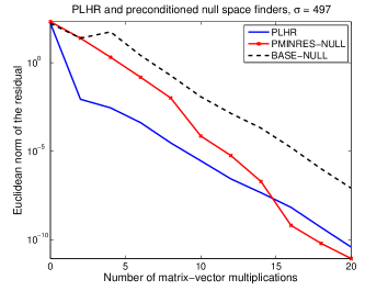
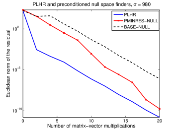
Fig. 1: A comparison of PLHR with preconditioned linear solvers for $(A-\lambda_{31}B)x=0$ (left) and $(A-\lambda_{66}B)x=0$ (right), where $\lambda_{31}\approx 497.5521$ and $\lambda_{66}\approx 979.7072$.

In Figure 1, we apply PLHR (Algorithm 1) and BASE-NULL to compute an eigenpair closest to the shift $\sigma=497$ and $\sigma=980$. These shift values target eigenpairs corresponding to the eigenvalues $\lambda_{31}\approx 497.5521$ and $\lambda_{66}\approx 979.7072$, respectively. Thus, BASE-NULL solves the homogeneous systems with matrices $A-\lambda_{31}B$ and $A-\lambda_{66}B$. We also plot convergence curves that correspond to the runs of PMINRES (denoted PMINRES-NULL) applied to the same singular systems. This gives us an opportunity to compare the convergence of PLHR to that of an optimal Krylov subspace method used as an idealized eigenvalue solver; see the discussion in Section 2.

To assess the convergence, for all schemes in Figure 1, we measure the norms of the residuals $\|Av^{(i)}-\lambda^{(i)}Bv^{(i)}\|$ of the eigenvalue problem. In the definition of the random perturbation based preconditioner $T$, we set $\epsilon=10^{-5}$.

Figure 1 shows that PLHR and BASE-NULL exhibit essentially the same convergence behavior. Additionally, at a number of initial steps, their convergence is similar to that of PMINRES-NULL. Thus, at least if the preconditioner is sufficiently strong, the approximations introduced into the idealized BASE-NULL to obtain PLHR do not significantly alter its convergence behavior. Moreover, the convergence is comparable to that of the optimal PMINRES-NULL.

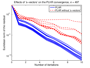
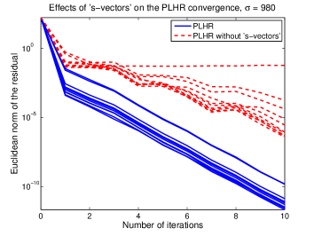
Fig. 2: The significance of “s-vectors” for the PLHR convergence. The PLHR algorithm with $\sigma=497$ (left) and $\sigma=980$ (right) is compared to its version without “s-vectors”. Each curve corresponds to a separate run with random initial guess and a preconditioner generated by a random SPD perturbation of $|A-\sigma B|^{-1}$ with $\epsilon=10^{-5}$.

Next, we would like demonstrate the effects of the vectors $s^{(i)}$ introduced into the PLHR trial subspaces (11). These subspaces can be viewed as the LOBPCG-like subspaces, spanned by $v^{(i)}$, $w^{(i)}$, and $p^{(i)}$, extended by the additional vector. Therefore, a natural question is whether the occurrence of the new “s-vectors” has any impact on the convergence of the proposed scheme.

Figure 2 compares the PLHR iteration in Algorithm 1 to its variant where the “s-vectors” are not included into the trial subspaces, i.e., (11) are spanned only by $v^{(i)}$, $w^{(i)}$, and $p^{(i)}$. We perform $10$ runs of both versions of the algorithm, so that each curve in Figure 2 represents a separate execution with a random initial guess. As in the previous example, we consider shifts $\sigma=497$ and $\sigma=980$. For each run, the preconditioners are given by random SPD perturbations of $|A-\sigma B|^{-1}$ with $\epsilon=10^{-5}$.

One can observe from Figure 2 that PLHR demonstrates a stable linear convergence at all runs regardless of the initial guess and a particular instance of the preconditioner. At the same time, despite the high preconditioning quality, the absence of “s-vectors” makes the method highly unstable, with a slower or stagnant convergence pattern. Therefore, the presence of $s^{(i)}$ in (11) is important. Such a behavior is consistent with the fact that linear solver (3) generally does not converge if $s$-vectors, defined as $T\left(A-\lambda_{q}B\right)Tr^{(i)}$, are removed from the iterative scheme.

Another new feature incorporated into PLHR is the $T$-harmonic RR procedure presented in Section 3.1. Similar to the above, we would like to address the question of whether any advantage is gained by the $T$-harmonic approach compared, e.g., to the standard harmonic RR [22]. To answer this question, let us compare the PLHR algorithm to its variant where the $T$-harmonic projection is replaced by the standard harmonic RR, whereas the same SPD (AV) preconditioner is used to generate the trial subspaces.

Since PLHR with a standard harmonic RR no longer requires the preconditioner to be SPD, we are also interested in the case where $T$ is indefinite, i.e., the preconditioner is an approximation of the “shift-and-invert” operator $(A-\sigma B)^{-1}$. For this reason, let us consider a variant of PLHR with an indefinite $T\approx(A-\sigma B)^{-1}$, combined with the standard harmonic RR.

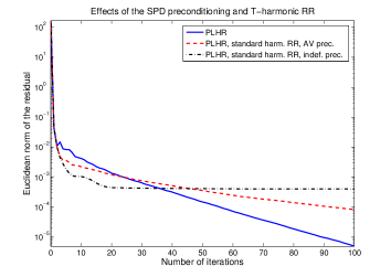
Fig. 3: Effects of the SPD AV preconditioning and $T$-harmonic RR; $\sigma=980$. Preconditioners generated by a random SPD perturbation of $|A-\sigma B|^{-1}$ (for the AV preconditioner) and of $(A-\sigma B)^{-1}$ (for the indefinite preconditioner) with $\epsilon=10^{-4}$ (left) and $\epsilon=10^{-3}$ (right).

Figure 3 illustrates the collective impact of the $T$-harmonic RR and AV preconditioning on the convergence of the new eigensolver. Here, we set $\sigma=980$ and apply all the three PLHR variants to compute the corresponding eigenpair.

In contrast to our previous tests, we now consider preconditioners of different quality. In particular, in Figure 3 (left) we set $\epsilon=10^{-4}$, whereas in Figure 3 (right) we choose $\epsilon=10^{-3}$, which gives weaker preconditioners. As previously, the AV preconditioning is obtained by perturbing $|A-\sigma B|^{-1}$. The indefinite preconditioner is generated in a similar manner by a random perturbation $E$ of $(A-\sigma B)^{-1}$, i.e., $T=(A-\sigma B)^{-1}+E$, where $\|E\|\leq\epsilon\|(A-\sigma B)^{-1}\|$. In our tests, the same SPD perturbation $E$ is used for both the AV and indefinite preconditioners to maintain a similar preconditioning quality.

Figure 3 (left) suggests that if a sufficiently strong preconditioner is at hand then neither the $T$-harmonic projection nor the SPD preconditioning lead to any significant improvement. In this case, the fastest convergence is attained by the version of PLHR with the standard harmonic RR and indefinite preconditioner. However, if preconditioning is not as strong, then the use of the SPD AV preconditioners along with the $T$-harmonic RR procedure becomes crucial. As can be seen in Figure 3 (right), the original PLHR version given by Algorithm 1 is the only scheme that is able to maintain convergence under the degraded preconditioning quality. Note that, in this example, the convergence of PLHR iterations could be preserved for values of $\epsilon$ up to $10^{-2}$. For $\epsilon=10^{-2}$, the convergence behavior of all methods is similar to that in Figure 3 (right), though with an increased iteration count due to preconditioning deterioration.

The case where the preconditioner is only of a moderate quality is not uncommon in realistic applications, especially if the wanted eigenpairs are located deeper in the spectrum’s interior. Thus, the decrease in the sensitivity to deterioration of the preconditioning quality, demonstrated by PLHR in Figure 3 (right), is of a practical interest. In the remaining experiments, we reaffirm this finding on the example of several model problems for which AV preconditioners can be constructed in practice.

6.2 A model problem: the finite-difference (FD) Laplacian

Let us consider the same continuous problem (23), but now apply a standard 5-point FD discretization with step $h=2^{-7}$. This gives an eigenvalue problem $Lv=\lambda v$, where $A\equiv L$ is a discrete Laplacian of size $n=16,129$.

We are interested in computing a subset of eigenvalues closest to the shift $\sigma$ using the block PLHR iteration. Since $L$ is SPD, we employ the real arithmetic version of BPLHR in Algorithm 3. In contrast to the previous example, where an artificial preconditioner has been constructed, we now utilize the practical SPD preconditioner $T\approx|L-\sigma I|^{-1}$ introduced in [35]. For convenience, we state this preconditioning procedure in Algorithm 4 of Appendix A.

The objective of the current experiment is two-fold. On the one hand, we would like to compare BPLHR to a well-established solution scheme, such as the BGD method. On the other hand, similar to our previous test, we are interested in demonstrating effects of the $T$-harmonic extraction and AV preconditioning on the eigensolver convergence.

We consider two preconditioning options for the BGD algorithm. The first approach is exactly the same MG AV preconditioner [35] (Algorithm 4 of Appendix A) as the one used in the BPLHR algorithm, i.e., $T\approx|L-\sigma I|^{-1}$ and it is SPD. The second preconditioner is given by a standard MG solve [4, 33] for the shifted matrix $L-\sigma I$ (see Algorithm 5 of Appendix A), which corresponds to an indefinite “shift-and-invert” type preconditioner $T\approx(L-\sigma I)^{-1}$.

The preconditioners in Algorithms 4 and 5 are of the same nature. They represent a standard MG V-cycle, with the difference that the former is applied to solve the SPD system $|L-\sigma I|w=r$ [35], whereas the latter seeks to approximate the solution of the indefinite $(L-\sigma I)w=r$. Note that preconditioners stronger than Algorithm 5 are available for the indefinite matrix $L-\sigma I$, such as, e.g., in [21]. However, due to the algorithmic similarity to the employed MG AV preconditioner, for demonstration purposes, we use Algorithm 5 as a reference indefinite MG preconditioner.

In order to ensure a comparable (in terms of the approximate solves for the corresponding linear systems $|L-\sigma I|w=r$ and $(L-\sigma I)w=r$) preconditioning quality in the two variants of BGD, we require that the coarsest grid problems are of the same size (225 by 225) and that the same smoothing schemes (a single step of Richardson’s iterations) are used on every level. Note that the computational costs of both preconditioners is essentially the same, with the AV preconditioner performing slightly more arithmetic operations because of the polynomial approximations of the absolute value operators on intermediate levels. However, these additional expenses are negligible relative to the overall preconditioning cost.

Recall that at every iteration the BGD algorithm expands the search subspace with a set of preconditioned residuals. Thus, an increased amount of memory is required by the method at every new step. This is in contrast to the BPLHR algorithm, where the requested storage size is fixed at every iteration. In particular, in our implementation, BPLHR has to store at most $12k$ vectors corresponding to $Z(=[V^{(i)},W^{(i)},S^{(i)},P^{(i)}])$, $AZ$, and $T(A-\sigma B)Z$.

To maintain the same memory requirement in BGD, we restart the method once the size $m$ of its search subspace becomes sufficiently large, reaching some prespecified $m_{\max}$. In this case, we collapse the search subspace, so that it only contains $k$ available eigenvector approximations. Since in standard BGD implementations each iteration of the method stores the search subspace $Z_{m}$ together with the block $AZ_{m}$ (i.e., up to $2m$ vectors total), we want $2m$ not to exceed $12k$. Hence, to ensure the same memory requirement for BPLHR and BGD, we set $m_{\max}=6k$. This maximum size of the BGD subspace is somewhat larger than the size of the trial subspaces in BPLHR which is $4k$. Nevertheless, as we demonstrate below, BPLHR can be more robust, even though the extraction is performed with respect to the smaller subspaces.

While our main focus is on the comparison of the BPLHR and BGD methods, we are also interested in the question of how much the AV preconditioning affects the eigensolver’s convergence and if any benefit is received from the $T$-harmonic RR. For this reason, along with the original BPLHR version in Algorithm 3, we also consider its versions based on the standard harmonic RR with the AV and indefinite preconditioning options, similar to the previous section. Here, the AV and indefinite preconditioning strategies are based on the MG schemes in Algorithms 4 and 5, respectively.

			Shifts ($\sigma$)
Iter. scheme	Prec.	RR	400	450	500	550	600	650	700
BPLHR	AV	$T$-harm.	57	81	68	133	117	190	278
BPLHR	AV	harm.	563	-	493	635	-	-	-
BPLHR	Indef.	harm.	30	40	45	-	59	338	424
BGD	AV	harm.	209	-	533	-	493	-	-
BGD	Indef.	harm.	36	46	57	-	376	763	-

Table 1: Iteration numbers required by different eigensolvers to converge to 10 eigenpairs of the 2D FD Laplacian closest to the shifts $\sigma$; “-” corresponds to the cases where no convergence was reached within $1000$ iteration; $n=16,129$. The AV and indefinite preconditioners are given by Algorithms 4 and 5, respectively.

In Table 1 we report the numbers of iterations required by different eigensolvers to converge to 10 eigenpairs closest to the given shift. The schemes were compared for a number of shifts in the range from $400$ to $700$. The convergence tolerance for the residual norms was set to $10^{-6}$ and the same initial guess was used for each run corresponding to the same $\sigma$. Since the real arithmetic version of BPLHR is invoked, according to the discussion in Section 4.1, we increase the block size by one, i.e., apply Algorithm 3 with $k=11$, but track the convergence only of the ten wanted eigenpairs. The maximum size $m_{\max}$ of the BGD search subspace is $66$.

Table 1 shows that the BPLHR algorithm (i.e., the original version with the AV preconditioner and $T$-harmonic RR) is robust with respect to the choice of the shift. It is the only method among the compared schemes that was able to converge all eigenpairs for each $\sigma$ in the prescribed range. Note that the $T$-harmonic extraction is crucial—its replacement by the standard harmonic approach (while preserving the same AV preconditioner) resulted in a significant increase of the iteration count or a total loss of convergence. The demonstrated results also suggest that the standard harmonic extraction leads to more satisfactory results if an indefinite preconditioner is employed. However, this combination was still unable to maintain convergence for all shifts and required a noticeably larger amount of iterations for $\sigma\geq 650$.

Regardless of the choice of the preconditioner, both BGD based schemes fail to converge for a number of shift values. Note that for smaller values of $\sigma$ ($400$ to $500$), BGD with the indefinite preconditioning gives the lowest number of iterations. However, as $\sigma$ increases, either the iteration count grows dramatically or the convergence of the method is lost.

As has been discussed in Section 4, in the reported runs, the cost of each BPLHR iteration is dominated by 2 matrix-block multiplications and 4 block preconditioning operations. This is clearly more expensive than, e.g., in the BGD method, where only one of each is needed. However, as seen in Table 1, BGD fails to maintain convergence under the given memory constraint, whereas BPLHR succeeds, i.e., the increased iteration cost results in an improved robustness of the overall computation.

It is well known (e.g., [5, 35]) that the the increase of $\sigma$ generally leads to the deterioration of the MG solves for $|L-\sigma I|$ and $L-\sigma I$ in Algorithms 4 and 5. Therefore, the observed shift robustness of BPLHR indicates that the method is more stable with respect to the loss of preconditioning quality compared to the other methods tested. Remarkably, as $\sigma$ increases, the number of BPLHR iterations does not grow too fast.

			Shifts ($\sigma$)
Iter. scheme	Prec.	RR	800	900	1000	1100	1200	1300	1400
BPLHR	AV	$T$-harm.	270	168	177	344	365	363	192
BPLHR	AV	harm.	590	417	377	625	437	217	287
BPLHR	Indef.	harm.	-	-	-	-	-	-	-
BGD	AV	harm.	331	305	356	666	509	481	443
BGD	Indef.	harm.	230	818	837	-	-	-	-

Table 2: Iteration numbers required by different eigensolvers to converge to 20 eigenpairs of the 2D FD Laplacian closest to the shifts $\sigma$; “-” corresponds to the cases where no convergence was reached within $1000$ iteration; $n=16,129$. The AV and indefinite preconditioners are given by Algorithms 4 and 5, respectively.

In Table 2 we report a similar experiment, where the number $k$ of targeted eigenpairs has been increased to $20$; the maximum size of the BGD search subspace is set to $126$. The range of shifts is between 800 and 1400. Again, we can see that BPLHR was able to converge for all values of $\sigma$ and in most cases exhibited the lowest iteration count. The schemes based on BPLHR and BGD with the indefinite MG preconditioning failed to provide satisfactory convergence. We relate it to a deteriorated quality of the INV-MG preconditioner in Algorithm 5 for larger shift values. In particular, this shows that the AV preconditioning is more robust if the targeted eigenpairs are deeper in the spectrum’s interior. Also, note that the increased block size, compared to the case in Table 1, allows PLHR to handle larger values of $\sigma$, due to the corresponding increase of the size of the trial subspaces.

$\omega$	6	7	8	9
$\#$ iterations	41	42	43	42

Table 3: Mesh independence of the BPLHR algorithm with the MG AV preconditioner [35] for the 2D FD Laplacian. The mesh parameter is given by $h=1/(2^{\omega}+1)$. Four eigenpairs corresponding to the eigenvalues closest to $\sigma=400$ are computed.

It was demonstrated in [35] that, in the context of solving linear systems $(L-\sigma I)w=r$, the MG AV preconditioner in Algorithm 4 leads to a mesh-independent convergence of an iterative solver. In Table 3, we show that this property also holds if the same AV preconditioning is combined with the BPLHR scheme for computing interior eigenpairs. In particular, we decrease the mesh size $h=1/(2^{\omega}+1)$ by varying the parameter $\omega$ between $6$ and $9$, and observe that the number of steps required to obtain the residual norm of $10^{-4}$ is about the same for each run. Here, in order to mitigate the effects of deflation, we compute fewer ($k=4$) eigenpairs. The shift $\sigma$ is set to $400$.

6.3 Interior eigenpairs of the Kohn–Sham Hamiltonians

In this concluding set of experiments we apply BPLHR to several Hermitian matrices that arise in the context of electronic structure calculations. These matrices correspond to plane wave discretizations of the Hamiltonian operators in the framework of the Kohn–Sham (KS) density functional theory [17]. All tests are performed within the KSSOLV package [41]—a matlab toolbox for solving the KS equations.

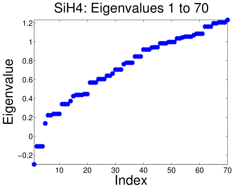
(a) SiH4.

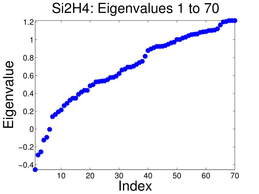
(b) Si2H4.

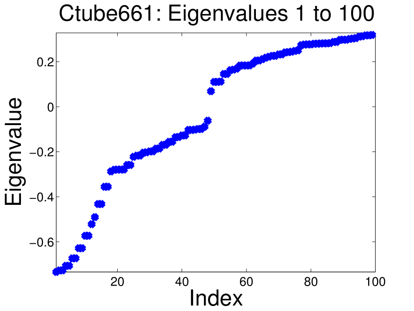
(c) Ctube661.

Fig. 4: Parts of spectra of the Hamiltonian matrices.

We consider three model systems of particles: the silane (SiH2) and planar singlet silysilylene (Si2H4) molecules, and a carbon nanotube (Ctube661). For each system, we set up the corresponding KS equations, which give a nonlinear eigenvalue problem. The problem is discretized and then solved using a self-consistent field iteration. As a result of this iteration, the nonlinear operator (Hamiltonian) of the discrete KS problem converges to a matrix which represents the Hamiltonian for the converged electron density. The spectrum of this converged Hamiltonian describes the electronic structure of the underlying system. Its eigenvalues represent different energy levels and the eigenvectors define the associated wavefunctions, or orbitals.

In our tests, we are interested in computing interior eigenpairs of the converged Hamiltonians corresponding to the three model systems. In particular, for each problem, we would like to compare the convergence of the BPLHR algorithm to that of BGD, where the schemes are applied to find $k$ eigenpairs around a given shift $\sigma$. Throughout, we let $k$ be equal to $10$, i.e., ten eigenpairs closest to $\sigma$ are sought in every test. Since the Hamiltonians are complex, all our computations are performed in the complex arithmetic, i.e., Algorithm 2 is employed.

We use the Teter–Payne–Allan preconditioner developed in [32]. This preconditioning approach is known to be effective for eigenvalue computations in the context of the plane wave electronic structure analysis, and is readily available in KSSOLV. Although the preconditioner is more commonly used for computing a number of lowest eigenpairs, it can also be applied to the interior eigenvalue computations provided that the targeted eigenvalues are not too deep inside the spectrum. For example, combining the preconditioning of [32] with a (block) Davidson algorithm based on the harmonic extraction was suggested for computing interior eigenpairs in [12]. The BGD scheme used in this section is similar to this approach.

The preconditioner in [32] represents a diagonal matrix with positive entries. Hence, the preconditioning is SPD and its application is extremely fast. This is especially beneficial for the BPLHR algorithm, where additional preconditioning operations are needed to accomplish the $T$-harmonic extraction. Since the cost of the diagonal preconditioning is negligible, the total cost of each BPLHR iteration is dominated by two matrix-block multiplications. The similar consideration applies to the BGD algorithm, whose iteration cost is dominated by a single matrix-block product.

Following the discussion in the preceding subsection, we choose the restart parameter in BGD to be at least $6k=60$. In this case BGD and BPLHR have the same memory requirement. In some of our tests, however, we will allow BGD to construct search subspaces that are larger than $60$. For this reason, in order to distinguish between different subspace sizes, let us denote each BGD run by “BGD($m_{\max}$)”, where $m_{\max}$ specifies the corresponding restart parameter.

As previously, in order to address the effects of the $T$-harmonic extraction, we also consider the BPLHR variant with a standard harmonic RR procedure. It is combined with exactly the same SPD diagonal preconditioner [32] as the one used in BPLHR and BGD.

To discretize the three model Hamiltonians, we use the energy cut-off of 75 Ry for the SiH4 and Si2H4 systems, and 25 Ry for the carbon tube. This leads to the eigenvalue problems of size $n=11,019$ (for SiH4 and Si2H4) and $n=12,599$ (for Ctube661). The parts of spectrum that we are interested in for each of the three Hamiltonian matrices are plotted in Figure 4.

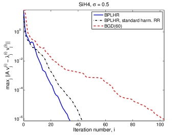
Fig. 5: Computing $10$ eigenpairs closest to $\sigma=0.5$ (left) and $\sigma=0.8$ (right) of the converged Hamiltonian of the SiH4 system; $n=11,019$.

Figure 5 shows the convergence of the three schemes for the SiH4 example. Here and below, we assess the convergence by monitoring the largest residual norm in the block. Note that in our experiments all the $10$ targeted pairs converge essentially at the same rate. Therefore, tracking only the largest norm is indicative of the convergence behavior of each eigenpair in the block.

It can be seen from Figure 5 that for both shifts, $\sigma=0.5$ (left) and $\sigma=0.8$ (right), the BPLHR algorithm results in almost a three times reduction in the number of iterations compared to BGD. Even though each BPLHR iteration is (roughly) twice as expensive as the BGD step, the overall decrease of the computational work is evident. Additionally, note that the BGD run in Figure 5 (right) requires more memory than BPLHR, i.e., BPLHR gives a faster convergence while consuming less storage. Our experiments below will make this observation yet more pronounced.

We can see from Figure 5 (left) that the introduction of the $T$-harmonic projection results in a minor improvement of the convergence for $\sigma=0.5$. In this case, the number of BPLHR iterations is only slightly decreased compared to its version with the standard harmonic RR. However, for the larger shift ($\sigma=0.8$) in Figure 5 (right) the situation is substantially different. The $T$-harmonic projection in BPLHR allows reducing the iteration count by more than a factor of two. Thus, the $T$-harmonic RR procedure makes the scheme less sensitive to the choice of the shift and more stable with respect to deterioration of the preconditioning quality. Note that this is consistent with our observations in the previous subsections.

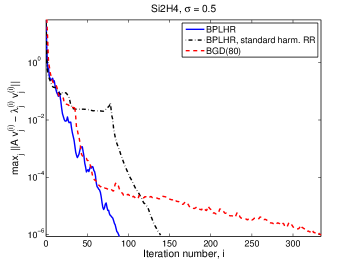
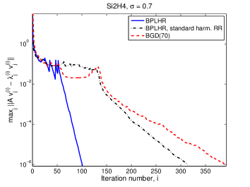
Fig. 6: Computing $10$ eigenpairs closest to $\sigma=0.5$ (left) and $\sigma=0.7$ (right) of the converged Hamiltonian of the Si2H4 system; $n=11,019$.

In Figure 6, we apply the eigensolvers to the Hamiltonian of the Si2H4 system. The targeted energy shifts are $\sigma=0.5$ (left) and $\sigma=0.7$ (right). In both cases, the BPLHR algorithm gives the smallest iteration count and a significant decrease of the overall computational work. For example, we can see around 4 time reduction in the number of iterations compared to BGD. The impact of the $T$-harmonic projection on the BPLHR convergence can be observed by comparing the method with its variant based on the standard harmonic RR. Similar to the previous test, note that BGD requires more memory than the BPLHR schemes.

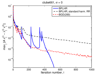
Fig. 7: Commuting $10$ eigenpairs closest to $\sigma=-0.25$ (left) and $\sigma=0$ (right) of the converged Hamiltonian of the carbon tube; $n=12,599$.

Our last experiment for the carbon tube is presented in Figure 7. In this example, the BPLHR algorithm is the only scheme that is able to reach convergence of the eigenpairs near the shift $\sigma=-0.25$ (left) and $\sigma=0$ (right). Remarkably, the BGD search subspaces are allowed to be 3 to 5 times larger than the BPLHR trial subspaces. Nevertheless, the increased memory consumption does not allow BGD to maintain the convergence, whereas the BPLHR algorithm computes the solution with a much tighter storage. The example also clearly demonstrates the importance of the $T$-harmonic RR. Substituting the procedure by the standard harmonic RR leads to the loss of convergence.

7 Conclusions

We have presented the Preconditioned Locally Harmonic Residual (PLHR) algorithm for computing interior eigenpairs closest to the shift $\sigma$. The method represents a preconditioned four-term recurrence and can be easily extended to the block case (BPLHR). It is equally applicable to the standard and generalized eigenvalue problems. The algorithm is based on the $T$-harmonic RR procedure, and does not require shift-and-invert or folded spectrum transformations.

The proposed approach has been tested for a number of model problems, including the Laplacian and Hamiltonian (arising from the density functional theory based electronic structure calculations) matrices. (B)PLHR has been shown to exhibit a lower sensitivity to the preconditioning quality and has been able to maintain convergence under stringent memory requirements.

A possible limitation of the method is given by the need to provide an HPD AV preconditioner. However, as demonstrated in the paper, such preconditioners are available for a number of important applications, such as the plane wave electronic structure calculations. In the case where an AV preconditioner is unavailable, one can use the algorithm version with the standard harmonic RR instead of the proposed $T$-harmonic scheme. However, we anticipate that the (B)PLHR approach would greatly benefit from further progress in developing efficient AV preconditioning techniques.

Appendix A The AV-MG and INV-MG preconditioners

The idea behind the AV-MG preconditioner is to apply the formal MG V-cycle to the system $|L-\sigma I|w=r$, where $L$ is the Laplacian operator. A hierarchy of grids is introduced, and at each level $l$ the corresponding absolute value operator $|L_{l}-\sigma I_{l}|$ is approximated by some $B_{l}$. At finer grids, $B_{l}$ is chosen to be simply the Laplacian, i.e., $B_{l}=L_{l}$, whereas at coarser levels polynomial approximations are employed, so that $B_{l}=p_{m}(L_{l}-\sigma I_{l})$, where $m$ is a given degree of the polynomial. The (Richardson’s) smoothing is performed with respect to $B_{l}$. The restriction and prolongation are carried out in a standard way. The actual construction of $|L-\sigma I|$ appears only on the coarsest level, where the coarse grid solve is performed. The whole scheme is summarized in Algorithm 4. For more detail we refer the reader to [35].

Input: The residual $r_{l}$; parameters $\delta$, $\nu$, and $m$; Output: $w_{l}\approx|L_{l}-I_{l}|^{-1}r_{l}$;

1:  Set $B_{l}=L_{l}$ if $\sqrt{\sigma}h_{l}<\delta$. Otherwise define $B_{l}$ as a polynomial approximation $p_{m}(L_{l}-\sigma I_{l})$ of $|L_{l}-\sigma I_{l}|$, where $m$ is the degree of the polynomial.

2:  Presmoothing. Apply $\nu$ smoothing steps, $\nu\geq 1$:

$$w_{l}^{(i+1)}=w_{l}^{(i)}+M_{l}^{-1}(r_{l}-B_{l}w_{l}^{(i)}),\ i=0,\ldots,\nu-1,\ w_{l}^{(0)}=0,$$

where $M_{l}$ defines a smoother on level $l$. Set $w_{l}^{pre}=w_{l}^{(\nu)}$.

3:  Coarse grid correction. Restrict ($R_{l-1}$) $r_{l}-B_{l}w_{l}^{pre}$ to the grid $l-1$, recursively apply AV-MG, and prolongate ($P_{l}$) back to the fine grid. This delivers the coarse grid correction added to $w_{l}^{pre}$:

$$w_{l-1}=\left\{\begin{array}[]{ll}\displaystyle\left|L_{0}-\sigma I_{0}\right|^{-1}R_{0}\left(r_{1}-B_{1}w_{1}^{pre}\right),&l=1,\\ \displaystyle\mbox{AV-MG}\left(R_{l-1}\left(r_{l}-B_{l}w_{l}^{pre}\right)\right),&l>1;\end{array}\right.$$

$$w_{l}^{cgc}=w_{l}^{pre}+P_{l}w_{l-1}.$$

4:  Postsmoothing. Apply $\nu$ smoothing steps:

(24) $$w_{l}^{(i+1)}=w_{l}^{(i)}+M_{l}^{-*}(r_{l}-B_{l}w_{l}^{(i)}),\ i=0,\ldots,\nu-1,\ w_{l}^{(0)}=w_{l}^{cgc},$$

where $M_{l}$ and $\nu_{l}$ are the same as in step 2. Return $w_{l}=w_{l}^{post}=w_{l}^{(\nu)}$.

Algorithm 4 AV-MG($r_{l}$): the MG AV preconditioner

The INV-MG preconditioner represents a standard $V$-cycle for system $(L-\sigma I)w=r$ and results in an indefinite preconditioner. The preconditioning scheme is stated in Algorithm 5. Note that, in this paper, the choice of the main MG components, such as smoothers, restriction and prolongation operators, for Algorithm 5 is identical to AV-MG in Algorithm 4.

Input: The residual $r_{l}$; $\nu$; Output: $w_{l}\approx(L_{l}-I_{l})^{-1}r_{l}$;

1:  Presmoothing. Apply $\nu$ smoothing steps, $\nu\geq 1$:

$$w_{l}^{(i+1)}=w_{l}^{(i)}+M_{l}^{-1}(r_{l}-(L_{l}-\sigma I_{l})w_{l}^{(i)}),\ i=0,\ldots,\nu-1,\ w_{l}^{(0)}=0,$$

where $M_{l}$ defines a smoother on level $l$. Set $w_{l}^{pre}=w_{l}^{(\nu)}$.

2:  Coarse grid correction. Restrict ($R_{l-1}$) $r_{l}-(L_{l}-\sigma I_{l})w_{l}^{pre}$ to the grid $l-1$, recursively apply INV-MG, and prolongate ($P_{l}$) back to the fine grid. This delivers the coarse grid correction added to $w_{l}^{pre}$:

$$w_{l-1}=\left\{\begin{array}[]{ll}\displaystyle\left(L_{0}-\sigma I_{0}\right)^{-1}R_{0}\left(r_{1}-B_{1}w_{1}^{pre}\right),&l=1,\\ \displaystyle\mbox{AV-MG}\left(R_{l-1}\left(r_{l}-(L_{l}-\sigma I_{l})w_{l}^{pre}\right)\right),&l>1;\end{array}\right.$$

$$w_{l}^{cgc}=w_{l}^{pre}+P_{l}w_{l-1}.$$

3:  Postsmoothing. Apply $\nu$ smoothing steps:

$$w_{l}^{(i+1)}=w_{l}^{(i)}+M_{l}^{-*}(r_{l}-(L_{l}-\sigma I_{l})w_{l}^{(i)}),\ i=0,\ldots,\nu-1,\ w_{l}^{(0)}=w_{l}^{cgc},$$

where $M_{l}$ and $\nu_{l}$ are the same as in step 2. Return $w_{l}=w_{l}^{post}=w_{l}^{(\nu)}$.

Algorithm 5 INV-MG($r_{l}$): the MG preconditioner

References

- [1] O. Axelsson, Iterative solution methods, Cambridge University Press, New York, NY, 1994.
- [2] Z. Bai, J. Demmel, J. Dongarra, A. Ruhe, and H. van der Vorst, eds., Templates for the solution of algebraic eigenvalue problems, Society for Industrial and Applied Mathematics (SIAM), Philadelphia, PA, 2000.
- [3] A. Borzì and G. Borzì, Algebraic multigrid methods for solving generalized eigenvalue problems, Int. J. Numer. Meth. Engng., 65 (2005), pp. 1186–1196.
- [4] W. L. Briggs, V. E. Henson, and S. F. McCormick, A Multigrid Tutorial, Society for Industrial and Applied Mathematics, 2nd ed., 2000.
- [5] H. C. Elman, O. G. Ernst, and D. O’Leary, A multigrid method enhanced by Krylov subspace iteration for discrete Helmholtz equations, SIAM J. Sci. Comput., 23 (2001), pp. 1291–1315.
- [6] H. Fang and Y. Saad, A filtered Lanczos procedure for extreme and interior eigenvalue problems, SIAM J. Sci. Comput., 34 (2012), pp. A2220–A2246.
- [7] G. H. Golub and C. F. V. Loan, Matrix Computations, The Johns Hopkins University Press, 3d ed., 1996.
- [8] G. H. Golub and Q. Ye, An inverse free preconditioned Krylov subspace method for symmetric generalized eigenvalue problems, SIAM J. Sci. Comput., 24 (2002), pp. 312–334.
- [9] A. Greenbaum, Iterative Methods for Solving Linear Systems, SIAM, 1997.
- [10] U. Hetmaniuk, A Rayleigh quotient minimization algorithm based on algebraic multigrid, Numer. Linear Algebra Appl., 14 (2007), pp. 563–580.
- [11] Z. Jia, Refined iterative algorithms based on Arnoldi’s process for large unsymmetric eigenproblems, Linear Algebra and its Applications, 259 (1997), pp. 1–23.
- [12] G. Jordan, M. Marsman, Y.-S. Kim, and G. Kresse, Fast iterative interior eigensolver for millions of atoms, J. Comput. Phys., 231 (2012), pp. 4836–4847.
- [13] A. V. Knyazev, Computation of eigenvalues and eigenvectors for mesh problems: algorithms and error estimates, Dept. Numerical Math. USSR Academy of Sciences, Moscow, 1986. (In Russian).
- [14] A. V. Knyazev, Preconditioned eigensolvers - an oxymoron?, Electronic Transactions on Numerical Analysis, 7 (1998), pp. 104–123.
- [15] A. V. Knyazev, Toward the optimal preconditioned eigensolver: locally optimal block preconditioned conjugate gradient method, SIAM Journal on Scientific Computing, 23 (2001), pp. 517–541.
- [16] A. V. Knyazev, M. E. Argentati, I. Lashuk, and E. E. Ovtchinnikov, Block locally optimal preconditioned eigenvalue xolvers (BLOPEX) in hypre and PETSc, SIAM Journal on Scientific Computing, 25 (2007), pp. 2224–2239.
- [17] W. Kohn and L. Sham, Self-consistent equations including exchange and correlation effects, Phys. Rev., 140 (1965), pp. A1133–A1138.
- [18] G. Kresse and J. Furthmüller, Efficiency of ab-initio total energy calculations for metals and semiconductors using a plane-wave basis set, Computational Materials Science, 6 (1996), pp. 15–50.
- [19] D. Kushnir, M. Galun, and A. Brandt, Efficient multilevel eigensolvers with applications to data analysis tasks, IEEE Trans. Pattern. Anal. Mach. Intell., 32 (2010), pp. 1377–1391.
- [20] I. Livshits, An algebraic multigrid wave-ray algorithm to solve eigenvalue problems for the Helmholtz operator, Numer. Linear Algebra Appl., 11 (2004), pp. 229–239.
- [21] I. Livshits and A. Brandt, Accuracy properties of the wave-ray multigrid algorithm for Helmholtz equations, SIAM J. on Sci. Comput., 28 (2006), pp. 1228–1251.
- [22] R. B. Morgan, Computing interior eigenvalues of large matrices, Linear Algebra Appl., 154–156 (1991), pp. 289–309.
- [23] R. B. Morgan and M. Zeng, Harmonic projection methods for large non-symmetric eigenvalue problems, Numer. Linear Algebra Appl., 5 (1998), pp. 33–55.
- [24] C. C. Paige, B. N. Parlett, and H. A. van der Vorst, Approximate solutions and eigenvalue bounds from krylov subspaces, Numer. Linear Algebra Appl., 2 (1995), pp. 115–133.
- [25] C. C. Paige and M. A. Saunders, Solution of sparse indefinite systems of linear equations, SIAM Journal on Numerical Analysis, 12 (1975), pp. 617–629.
- [26] B. N. Parlett, The symmetric eigenvalue problem, vol. 20 of Classics in Applied Mathematics, Society for Industrial and Applied Mathematics (SIAM), Philadelphia, PA, 1998. Corrected reprint of the 1980 original.
- [27] Y. Saad, Iterative Methods for Sparse Linear Systems, SIAM, Philadelpha, PA, 2003.
- [28] Y. Saad, Numerical Methods for Large Eigenvalue Problems- classics edition, SIAM, Philadelpha, PA, 2011.
- [29] T. SAKURAI and H. TADANO, Cirr: a rayleigh-ritz type method with contour integral for generalized eigenvalue problems, Hokkaido Mathematical Journal, 36 (2007), pp. 745–757.
- [30] G. L. G. Sleijpen and H. A. V. der Vorst, A Jacobi–Davidson Iteration Method for Linear Eigenvalue Problems, SIAM Journal on Matrix Analysis and Applications, 17 (1996), pp. 401–425.
- [31] G. W. Stewart, Matrix algorithms. Vol. II, SIAM, Philadelpha, PA, 2001.
- [32] M. P. Teter, M. C. Payne, and D. C. Allan, Solution of Schrödinger’s equation for large systems, Physical Review B, 40 (1989), pp. 12255–12263.
- [33] U. Trottenberg, C. W. Oosterlee, and A. Schüller, Multigrid, Academic Press, 2001.
- [34] E. Vecharynski, Preconditioned Iterative Methods for Linear Systems, Eigenvalue and Singular Value Problems. PhD thesis, University of Colorado Denver, 2011.
- [35] E. Vecharynski and A. V. Knyazev, Absolute value preconditioning for symmetric indefinite linear systems, SIAM J. Sci. Comput., 35 (2013), pp. A696–A718.
- [36] C. Vömel, A note on harmonic Ritz values and their reciprocals, Numer. Linear Algebra Appl., 17 (2010), pp. 97–108.
- [37] L. W. Wang and J. Li, First-principles thousand-atom quantum dot calculations, Phys. Rev. B, 69 (2004), p. 153302.
- [38] L. W. Wang and A. Zunger, Local-density-derived semiempirical pseudopotentials, Phys. Rev. B, 51 (1995), pp. 17398–17416.
- [39] , Linear combination of bulk bands method for large-scale electronic structure calculations on strained nanostructures, Phys. Rev. B, 59 (1999), pp. 15806–15818.
- [40] D. Wood and A. Zunger, A new method for diagonalising large matrices, Journal of Physics A: Mathematical and General, 18 (1985), p. 1343.
- [41] C. Yang, J. Meza, B. Lee, and L.-W. Wang, KSSOLV—a MATLAB toolbox for solving the Kohn-Sham equations, ACM Trans. Math. Softw., 36 (2009), pp. 10:1–10:35.
- [42] D. M. Young and K. C. Jea, Generalized conjugate-gradient acceleration of nonsymmetrizable iterative methods, Linear Algebra and its Applications, 34 (1980), pp. 159–194.