Learning From Ordered Sets and Applications in Collaborative Ranking

Abstract

Ranking over sets arise when users choose between groups of items. For example, a group may be of those movies deemed $5$ stars to them, or a customized tour package. It turns out, to model this data type properly, we need to investigate the general combinatorics problem of partitioning a set and ordering the subsets. Here we construct a probabilistic log-linear model over a set of ordered subsets. Inference in this combinatorial space is highly challenging: The space size approaches $(N!/2)6.93145^{N+1}$ as $N$ approaches infinity. We propose a split-and-merge Metropolis-Hastings procedure that can explore the state-space efficiently. For discovering hidden aspects in the data, we enrich the model with latent binary variables so that the posteriors can be efficiently evaluated. Finally, we evaluate the proposed model on large-scale collaborative filtering tasks and demonstrate that it is competitive against state-of-the-art methods.

1 Introduction

Rank data has recently generated a considerable interest within the machine learning community, as evidenced in ranking labels [7, 21] and ranking data instances [5, 23]. The problem is often cast as generating a list of objects (e.g., labels, documents) which are arranged in decreasing order of relevance with respect to some query (e.g., input features, keywords). The treatment effectively ignores the grouping property of compatible objects [22]. This phenomenon occurs when some objects are likely to be grouped with some others in certain ways. For example, a grocery basket is likely to contain a variety of goods which are complementary for household needs and at the same time, satisfy weekly budget constraints. Likewise, a set of movies are likely to given the same quality rating according to a particular user. In these situations, it is better to consider ranking groups instead of individual objects. It is beneficial not only when we need to recommend a subset (as in the case of grocery shopping), but also when we just want to produce a ranked list (as in the case of watching movies) because we would better exploit the compatibility among grouped items.

This poses a question of how to group individual objects into subsets given a list of all possible objects. Unlike the situation when the subsets are pre-defined and fixed (e.g., sport teams in a particular season), here we need to explore the space of set partitioning and ordering simultaneously. In the grocery example we need to partition the stocks in the store into baskets and then rank them with respect to their utilities; and in the movie rating example we group movies in the same quality-package and then rank these groups according to their given ratings. The situation is somewhat related to multilabel learning, where our goal is to produce a subset of labels out of many for a given input, but it is inherently more complicated: not only we need to produce all subsets, but also to rank them.

This paper introduces a probabilistic model for this type of situations, i.e., we want to learn the statistical patterns from which a set of objects is partitioned and ordered, and to compute the probability of any scheme of partitioning and ordering. In particular, the model imposes a log-linear distribution over the joint events of partitioning and ordering. It turns out, however, that the state-space is prohibitively large: If the space of complete ranking has the complexity of $N!$ for $N$ objects, then the space of partitioning a set and ordering approaches $(N!/2)6.93145^{N+1}$ in size as $N$ approaches infinity [11, pp. 396–397]. Clearly, the latter grows much faster than the former by an exponential factor of $6.93145^{N+1}$. To manage the exploration of this space, we design a split-and-merge Metropolis-Hastings procedure which iteratively visits all possible ways of partitioning and ordering. The procedure randomly alternates between the split move, where a subset is split into two consecutive parts, and the merge move, where two consecutive subsets are merged. The proposed model is termed Ordered Sets Model (OSM).

To discover hidden aspects in ordered sets (e.g., latent aspects that capture the taste of a user in his or her movie genre), we further introduce binary latent variables in a fashion similar to that of restricted Boltzmann machines (RBMs) [18]. The posteriors of hidden units given the visible rank data can be used as a vectorial representation of the data - this can be handy in tasks such as computing distance measures or visualisation. This results in a new model called Latent OSM.

Finally, we show how the proposed Latent OSM can be applied for collaborative filtering, e.g., when we need to take seen grouped item ratings as input and produce a ranked list of unseen item for each user. We then demonstrate and evaluate our model on large-scale public datasets. The experiments show that our approach is competitive against several state-of-the-art methods.

The rest of the paper is organised as follows. Section 2 presents the log-linear model over ordered sets (OSM) together with our main contribution – the split-and-merge procedure. Section 3 introduces Latent OSM, which extends the OSM to incorporate latent variables in the form of a set of binary factors. An application of the proposed Latent OSM for collaborative filtering is described in Section 4. Related work is reviewed in the next section, followed by the conclusions.

2 Ordered Set Log-linear Models

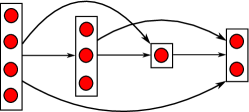
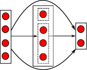
(a) OSM	(b)	(c)

Figure 1: (a) Ordered Set Model; (b) the split operator; and (c) the merge operator. The figure in (c) represents the result of a merge of the middle two subsets in (b). Conversely, the (b) figure can be considered as result of a splitting the middle subset of the (c) figure. Arrows represent the preference orders, not the causality or conditioning.

2.1 General Description

We first present an intuitive description of the problem and our solutions in modelling, learning and inference. Fig. 1(a) depicts the problem of grouping items into subsets (represented by a box of circles) and ordering these subsets (represented by arrows which indicate the ordering directions). This looks like a high-order Markov chain in a standard setting, and thus it is tempting to impose a chain-based distribution. However, the difficulty is that the partitioning of set into subsets is also random, and thus a simple treatment is not applicable. Recently, Truyen et al (2011) describe a model in this direction with a careful treatment of the partitioning effect. However, their model does not allow fast inference since we need to take care of the high-order properties.

Our solution is as follows. To capture the grouping and relative ordering, we impose on each group a subset potential function capturing the relations among compatible elements, and on each pair of subsets a ordering potential function. The distribution over the space of grouping and ordering is defined using a log-linear model, where the product of all potentials accounts for the unnormalised probability. This log-linear parameterization allows flexible inference in the combinatorial space of all possible groupings and orderings.

In this paper inference is carried out in a MCMC manner. At each step, we randomly choose a split or a merge operator. The split operator takes a subset at random (e.g., Fig. 1(c)) and uniformly splits it into two smaller subsets. The order between these two smaller subset is also random, but their relative positions with respect to other subsets remain unchanged (e.g., Fig. 1(b)). The merge operator is the reverse (e.g., converting Fig. 1(b) into Fig. 1(c)). With an appropriate acceptance probability, this procedure is guaranteed to explore the entire combinatorial space.

Armed with this sampling procedure, learning can be carried out using stochastic gradient techniques [25].

2.2 Problem Description

Given two objects $x_{i}$ and $x_{j}$, we use the notation $x_{i}\succ x_{j}$ to denote the expression of $x_{i}$ is ranked higher than $x_{j}$, and $x_{i}\sim x_{j}$ to denote the between the two belongs to the same group. Furthermore, we use the notation of $\mathit{X}=\left\{x_{1},x_{2},\ldots,x_{N}\right\}$ as a collection of $N$ objects. Assume that $X$ is partitioned into $T$ subsets $\left\{X_{t}\right\}_{t=1}^{T}$. However, unlike usual notion of partitioning of a set, we further posit an order among these subsets in which members of each subset presumably share the same rank. Therefore, our partitioning process is order-sensitive instead of being exchangeable at the partition level. Specifically, we use the indices $1,2,...,T$ to denote the decreasing order in the rank of subsets. These notations allow us to write the collection of objects $\mathit{X}=\left\{x_{1},\ldots,x_{N}\right\}$ as a union of $T$ ordered subsets:

$$\mathit{X}= X_{1}\bigcup X_{2}\ldots\bigcup X_{T}$$ (1)

where $\{\mathit{X}_{t}\}_{t=1}^{T}$ are non-empty subsets of objects so that $x_{i}\sim x_{j},\forall x_{i},x_{j}\in X_{t}$ $i\neq j,\forall t$.

As a special case when $T=N$, we obtain an exhaustive ordering among objects wherein each subset has exactly one element and there is no grouping among objects. This special case is equivalent with a complete ranking scenario. To illustrate the complexity of the problem, let us characterise the state-space, or more precisely, the number of all possible ways of partitioning and ordering governed by the above definition. Recall that there are $s\left(N,T\right)$ ways to divide a set of $N$ objects into $T$ partitions, where $s\left(N,T\right)$ denotes the Stirling numbers of second kind [20, p. 105]. Therefore, for each pair $(N,T)$, there are $s\left(N,T\right)T!$ ways to perform the partitioning with ordering. Considering all the possible values of $T$ give us the size of our model state-space:

$$\sum_{T=1}^{N}s\left(N,T\right)T! =\mbox{Fubini}\left(N\right)=\sum_{k=1}^{\infty}\frac{k^{N}}{2^{k+1}}$$ (2)

which is also known in combinatorics as the Fubini’s number [11, pp. 396–397]. This number grows super-exponentially and it is known that it approaches $N!/(2\left(\log 2\right)^{N+1})$ as $N\rightarrow\infty$ [11, pp. 396–397]. Taking the logarithm, we get $\log N!-(N+1)\log\log 2-\log 2$. As $\log\log 2<0$, this clearly grows faster than $\log N!$, which is the log of the size of the standard complete permutations.

2.3 Model Specification

Denote by $\Phi(X_{t})\in\mathbb{R}^{+}$ a positive potential function over a single subset $X_{t}$ and by $\Psi(X_{t}\succ X_{t^{\prime}})\in\mathbb{R}^{+}$a potential function over a ordered pair of subsets $\left(X_{t},X_{t^{\prime}}\right)$ where $t<t^{\prime}$. Our intention is to use $\Phi(X_{t})$ to encode the compatibility among all member of $X_{t}$, and $\Psi(X_{t}\succ X_{t^{\prime}})$ to encode the ordering properties between $X_{t}$ and $X_{t^{\prime}}$. We then impose a distribution over the collection of objects as:

$$P(X) = \frac{1}{Z}\Omega(X),\mbox{\qquad where}\,\,\Omega(X)=\prod_{t}\Phi(X_{t})\prod_{t^{\prime}>t}\Psi(X_{t}\succ X_{t^{\prime}})$$ (3)

and $Z=\sum_{X}\Omega(X)$ is the partition function. We further posit the following factorisation for the potential functions:

$$\Phi(X_{t}) = \prod_{i,j\in X_{t}|j>i}\varphi(x_{i}\sim x_{j});\mbox{\qquad\qquad}\Psi(X_{t}\succ X_{t^{\prime}})=\prod_{i\in X_{t}}\prod_{j\in X_{t^{\prime}}}\psi(x_{i}\succ x_{j})$$ (4)

where $\varphi(x_{i}\sim x_{j})\in\mathbb{R}^{+}$ captures the effect of grouping, and $\psi(x_{i}\succ x_{j})\in\mathbb{R}^{+}$ captures the relative ordering between objects $x_{i}$ and $x_{j}$. Hereafter, we shall refer to this proposed model as the Ordered Set Model (OSM).

2.4 Split-and-Merge MCMC Inference

In order to evaluate $P(X)$ we need to sum over all possible configurations of $X$ which is in the complexity of the Fubini($N$) over the set of $N$ objects (cf. Section 2.2, Eq. 2). We develop a Metropolis-Hastings (MH) procedure for sampling $P(X)$. Recall that the MH sampling involves a proposal distribution $Q$ that allows drawing a new sample $X^{\prime}$ from the current state $X$ with probability $Q(X^{\prime}|X)$. The move is then accepted with probability

$$P_{\mathsf{accept}}=\min\left\{1,l\times p\right\},\mbox{\qquad where}\,\,l=\frac{P(X^{\prime})}{P(X)}=\frac{\Omega(X^{\prime})}{\Omega(X)}\,\,\mbox{and}\,\,p=\frac{Q(X|X^{\prime})}{Q(X^{\prime}|X)}$$ (5)

To evaluate the likelihood ratio $l$ we use the model specification defined in Eq (3). We then need to compute the proposal probability ratio $p$. The key intuition is to design a random local move from $X$ to $X^{\prime}$ that makes a relatively small change to the current partitioning and ordering. If the change is large, then the rejection rate is high, thus leading to high cost (typically the computational cost increases with the step size of the local moves). On the other hand, if the change is small, then the random walks will explore the state-space too slowly.

We propose two operators to enable the proposal move: the split operator takes a non-singleton subset $X_{t}$ and randomly splits it into two sub-subsets $\{X_{t}^{1},X_{t}^{2}\}$, where $X_{t}^{2}$ is inserted right next to $X_{t}^{1}$; and the merge operator takes two consecutive subsets $\{X_{t},X_{t+1}\}$ and merges them. This dual procedure will guarantee exploration of all possible configurations of partitioning and ordering, given enough time (See Figure 1 for an illustration).

2.4.1 Split Operator

Assume that among the $T$ subsets, there are $T_{\mathsf{split}}$ non-singleton subsets from which we randomly select one subset to split, and let this be $X_{t}$. Since we want the resulting sub-subsets to be non-empty, we first randomly draw two distinct objects from $X_{t}$ and place them into the two subsets. Then, for each remaining object, there is an equal chance going to either $X_{t}^{1}$ or $X_{t}^{2}$. Let $N_{t}=|X_{t}|$, the probability of this drawing is $\left(N_{t}(N_{t}-1)2^{N_{t}-2}\right)^{-1}$. Since the probability that these two sub-subsets will be merged back is $T^{-1}$, the proposal probability ratio $p_{\mathsf{split}}$ can be computed as in Eq (6). Since our potential functions depend only on the relative orders between subsets and between objects in the same set, the likelihood ratio $l_{\mathsf{split}}$ due to the split operator does not depend on other subsets, it can be given as in Eq (7). This is because the members of $X_{t}^{1}$ are now ranked higher than those of $X_{t}^{2}$ while they are of the same rank previously.

$$p_{\mathsf{split}}=\frac{T_{\mathsf{split}}N_{t}(N_{t}-1)2^{N_{t}-2}}{T}$$ (6)

$$l_{\mathsf{split}}=\prod_{x_{i}\in X_{t}^{1}}\prod_{x_{j}\in X_{t}^{2}}\frac{\psi(x_{i}\succ x_{j})}{\varphi(x_{i}\sim x_{j})}$$ (7)

2.4.2 Merge Operator

For $T$ subsets, the probability of merging two consecutive ones will be $(T-1)^{-1}$ since there are $T-1$ pairs, and each pair can be merged in exactly one way. Let $T_{\mathsf{merge}}$ be the number of non-singleton subsets after the merge, and let $N_{t}$ and $N_{t+1}$be the sizes of the two subsets $X_{t}$ and $X_{t+1}$, respectively. Let $N_{t}^{*}=N_{t}+N_{t+1}$, the probability of recovering the state before the merge (by applying the split operator) is $\left(T_{\mathsf{merge}}N_{t}^{*}(N_{t}^{*}-1)2^{N_{t}^{*}-2}\right)^{-1}$. Consequently, the proposal probability ratio $p_{\mathsf{merge}}$ can be given as in Eq (8), and the likelihood ratio $l_{\mathsf{merge}}$ is clearly the inverse of the split case as shown in Eq (9).

$$p_{\mathsf{merge}}=\frac{T-1}{T_{\mathsf{merge}}N_{t}^{*}(N_{t}^{*}-1)2^{N_{t}^{*}-2}}$$ (8)

$$l_{\mathsf{merge}}=\prod_{x_{i}\in X_{t}}\prod_{x_{j}\in X_{t+1}}\frac{\varphi(x_{i}\sim x_{j})}{\psi(x_{i}\succ x_{j})}$$ (9)

Finally, the pseudo-code of the split-and-merge Metropolis-Hastings procedure for the OSM is presented in Algorithm 1.

1. Given an initial state $X$.

2. Repeat until convergence

2a. Draw a random number $\eta\in[0,1]$.
2b. If $\eta<0.5$ {Split}
	i. Randomly choose a non-singleton subset. ii. Split into two sub-subsets and insert one sub-subset right after the another. iii. Evaluate the acceptance probability $P_{\mathsf{accept}}$ using Eqs.(6,7,5). iv. Accept the move with probability $P_{\mathsf{accept}}$.
Else {Merge}
	i. Randomly choose two consecutive subsets. ii. Merge them in one, keeping the relative orders with other subsets unchanged. iii. Evaluate the acceptance probability $P_{\mathsf{accept}}$ using Eqs.(8,9,5). iv. Accept the move with probability $P_{\mathsf{accept}}$.
End

End

Algorithm 1 Pseudo-code of the split-and-merge Metropolis-Hastings for OSM.

2.5 Estimating Partition Function

To estimate the normalisation constant $Z$, we employ an efficient procedure called Annealed Importance Sampling (AIS) proposed recently [12]. More specifically, AIS introduces the notion of inverse-temperature $\tau$ into the model, that is $P(X|\tau)\propto\Omega(X)^{\tau}$.

Let $\{\tau_{s}\}_{s=0}^{S}$ be the (slowly) increasing sequence of temperature, where $\tau_{0}=0$ and $\tau_{S}=1$, that is $\tau_{0}<\tau_{1}...<\tau_{S}$. At $\tau_{0}=0$, we have a uniform distribution, and at $\tau_{S}=1$, we obtain the desired distribution. At each step $s$, we draw a sample $X^{s}$ from the distribution $P(X|\tau_{s-1})$ (e.g. using the split-and-merge procedure). Let $P^{*}(X|\tau)$ be the unnormalised distribution of $P(X|\tau)$, that is $P(X|\tau)=P^{*}(X|\tau)/Z(\tau)$. The final weight after the annealing process is computed as

$$w=\frac{P^{*}(X^{1}|\tau_{1})}{P^{*}(X^{1}|\tau_{0})}\frac{P^{*}(X^{2}|\tau_{2})}{P^{*}(X^{2}|\tau_{1})}...\frac{P^{*}(X^{S}|\tau_{S})}{P^{*}(X^{S}|\tau_{S-1})}$$ (10)

The above procedure is repeated $R$ times. Finally, the normalisation constant at $\tau=1$ is computed as $Z(1)\approx Z(0)\left(\sum_{r=1}^{R}w^{(r)}/R\right)$where $Z(0)=\mbox{Fubini}(N)$, which is the number of configurations of the model state variables $X$.

2.6 Log-linear Parameterisation and Learning

Here we assume that the model is in the log-linear form, that is $\varphi(x_{i}\sim x_{j})=\exp\left\{\sum_{a}\alpha_{a}f_{a}(x_{i},x_{j})\right\}$ and $\psi(x_{i}\succ x_{j})=\exp\left\{\sum_{b}\beta_{b}g_{b}(x_{i},x_{j})\right\}$, where $\left\{f_{a}(\cdot),\,g_{b}(\cdot)\right\}$ are sufficient statistics (or feature functions) and $\left\{\alpha_{a},\,\beta_{b}\right\}$ are free parameters.

Learning by maximising (log-)likelihood in log-linear models with respect to free parameters often leads to computing the expectation of sufficient statistics. For example, $\left\langle f_{a}(x_{i},x_{j})\right\rangle_{P(x_{i}\sim x_{j})}$ is needed in the gradient of the log-likelihood with respect to $\alpha_{a}$, where $P(x_{i}\sim x_{j})$ is the pairwise marginal. Unfortunately, computing $P(x_{i}\sim x_{j})$ is inherently hard, and running a full MCMC chain to estimate it is too expensive for practical purposes. Here we follow the stochastic approximation proposed in [25], in that we iteratively update parameters after very short MCMC chains (e.g., using Algorithm 1).

3 Introducing Latent Variables to OSMs

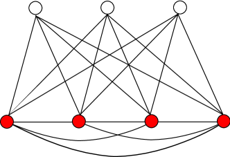
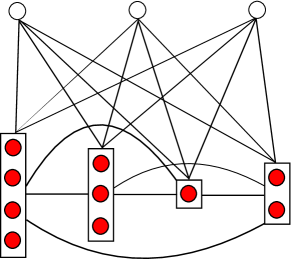
(a)		(b)

Figure 2: (a) A Semi-Restricted Boltzmann Machine representation of vectorial data: each shaded node represents a visible variable and empty nodes the hidden units. (b) A Latent OSM for representing ordered sets: each box represents a subset of objects.

In this section, we further extend the proposed OSM by introducing latent variables into the model. The latent variables serve multiple purposes. For example, in collaborative filtering, each person chooses only a small subset of objects, thus the specific choice of objects and the ranking reflects personal taste. This cannot be discovered by the standard OSM. Second, if we want to measure the distance or similarity between two ordered partitioned sets, e.g. for clustering or visualisation, it may be useful to first transform the data into some vectorial representation.

3.1 Model Specification

Denote by $\boldsymbol{h}=(h_{1},h_{2},...,h_{K})\in\{0,1\}^{K}$ the hidden units to be used in conjunction with the ordered sets. The idea is to estimate the posterior $P(h_{k}=1|X)$ - the probability that the $k^{\mbox{th}}$ hidden unit will be activated by the input $X$. Thus, the requirement is that the model should allow the evaluation of $P(h_{k}=1\mid X)$ efficiently. Borrowing from the Restricted Boltzmann Machine architecture [18, 24], we can extend the model potential function as follows:

$$\hat{\Omega}(X,\boldsymbol{h})=\Omega(X)\prod_{k}\Omega_{k}(X)^{h_{k}}$$ (11)

where $\Omega_{k}(X)$ admits the similar factorisation as $\Omega(X)$, i.e. $\Omega_{k}(X)=\prod_{t}\Phi_{k}(X_{t})\prod_{t^{\prime}>t}\Psi_{k}(X_{t}\succ X_{t^{\prime}})$, and

$$\Phi_{k}(X_{t}) = \prod_{i,j\in X_{t}|j>i}\varphi_{k}(x_{i}\sim x_{j});\quad\quad\Psi_{k}(X_{t}\succ X_{t^{\prime}})=\prod_{i\in X_{t}}\prod_{j\in X_{t^{\prime}}}\psi_{k}(x_{i}\succ x_{j})$$ (12)

where $\varphi_{k}(x_{i}\sim x_{j})$ and $\psi_{k}(x_{i}\succ x_{j})$ capture the events of tie and relative ordering between objects $x_{i}$ and $x_{j}$ under the presence of the $k^{\mbox{th}}$ hidden unit, respectively.

We then define the model with hidden variables as $P(X,\boldsymbol{h})=\hat{\Omega}(X,\boldsymbol{h})/Z$, where $Z=\sum_{X,\boldsymbol{h}}\hat{\Omega}(X,\boldsymbol{h})$. A graphical representation is given in Figure 2b. Hereafter, we shall refer to this proposed model as the Latent OSM.

3.2 Inference

The posteriors are indeed efficient to evaluate:

$$P(\boldsymbol{h}\mid X) = \prod_{k}P(h_{k}\mid X),\mbox{\quad where\,\,}P(h_{k}=1\mid X)=\frac{1}{1+\Omega_{k}(X)^{-1}}$$ (13)

Denote by $h_{k}^{1}$ as the shorthand for $h_{k}=1$, the vector $(P(h_{1}^{1}\mid X),P(h_{2}^{1}\mid X),...,P(h_{K}^{1}\mid X))$ can then be used as a latent representation of the configuration $X$.

The generation of $X$ given $\boldsymbol{h}$ is, however, much more involved as we need to explore the whole subset partitioning and ordering space:

$$P(X\mid\boldsymbol{h})=\frac{\hat{\Omega}(X,\boldsymbol{h})}{\sum_{X}\hat{\Omega}(X,\boldsymbol{h})}=\frac{\Omega(X)\prod_{k}\Omega_{k}(X)^{h_{k}}}{\sum_{X}\Omega(X)\prod_{k}\Omega_{k}(X)^{h_{k}}}$$ (14)

For inference, since we have two layers $X$ and $\boldsymbol{h}$, we can alternate between them in a Gibbs sampling manner, that is, sampling $X$ from $P(X\mid\boldsymbol{h})$ and then $\boldsymbol{h}$ from $P(\boldsymbol{h}\mid X)$. Since sampling from $P(\boldsymbol{h}\mid X)$ is straightforward, it remains to sample from $P(X|\boldsymbol{h})=\hat{\Omega}(X,\boldsymbol{h})/\sum_{X}\hat{\Omega}(X,\boldsymbol{h})$. Since $\hat{\Omega}(X,\boldsymbol{h})$ has the same factorisation structure into a product of pairwise potentials as $\Omega(X)$, we can employ the split-and-merge technique described in the previous section in a similar manner.

To see how, let $\hat{\varphi}(x_{i}\sim x_{j},\boldsymbol{h})=\varphi(x_{i}\sim x_{j})\prod_{k}\varphi_{k}(x_{i}\sim x_{j})^{h_{k}}$ and $\hat{\psi}(x_{i}\succ x_{j},\boldsymbol{h})=\psi_{k}(x_{i}\succ x_{j})\prod_{k}\psi_{k}(x_{i}\succ x_{j})^{h_{k}}$, then from Eqs.(4,11,12). We can see that $\hat{\Omega}(X,\boldsymbol{h})$ is now factorised into products of $\hat{\varphi}(x_{i}\sim x_{j},\boldsymbol{h})$ and $\hat{\psi}(x_{i}\succ x_{j},\boldsymbol{h})$ in the same way as $\Omega(X)$ into products of $\varphi(x_{i}\sim x_{j})$ and $\psi(x_{i}\succ x_{j})$:

$$\hat{\Omega}(X,\boldsymbol{h}) = \Omega(X)\prod_{k}\Omega_{k}(X)^{h_{k}}=\prod_{t}\hat{\Phi}(X_{t},\boldsymbol{h})\prod_{t^{\prime}>t}\hat{\Psi}(X_{t}\succ X_{t^{\prime}},\boldsymbol{h})$$

where

$$\hat{\Phi}(X_{t},\boldsymbol{h}) = \prod_{i,j\in X_{t}|j>i}\hat{\varphi}(x_{i}\sim x_{j},\boldsymbol{h});\quad\quad\hat{\Psi}(X_{t}\succ X_{t^{\prime}},\boldsymbol{h})=\prod_{i\in X_{t}}\prod_{j\in X_{t^{\prime}}}\hat{\psi}(x_{i}\succ x_{j},\boldsymbol{h})$$

Estimating the normalisation constant $Z$ can be performed using the AIS procedure described earlier (cf. Section 2.5), except that the unnormalised distribution $P^{*}(X|\tau)$ is given as:

$$P^{*}(X\mid\tau) =\sum_{\boldsymbol{h}}\hat{\Omega}(X,\boldsymbol{h})^{\tau}= \Omega(X)^{\tau}\prod_{k}\left(1+\Omega_{k}(X)^{\tau}\right)$$

which can be computed efficiently for each $X$.

For sampling $X^{s}$ from $P(X\mid\tau_{s-1})$, one way is to sample directly from the $P(X\mid\tau_{s-1})$ in a Rao-Blackwellised fashion (e.g. by marginalising over $\boldsymbol{h}$ we obtain the unnormalised $P^{*}(X|\tau)$). A more straightforward way is alternating between $X\mid\boldsymbol{h}$ and $\boldsymbol{h}\mid X$ as usual. Although the former would give lower variance, we implement the latter for simplicity. The remaining is similar to the case without hidden variables, and we note that the base partition function $Z(0)$ should be modified to $Z(0)=\mbox{Fubini}(N)2^{K}$, taking into account of $K$ binary hidden variables. A pseudo-code for the split-and-merge algorithm for Latent OSM is given in Algorithm 8.

1. Given an initial state $X$.

2. Repeat until convergence

2a. Sample $\boldsymbol{h}$ from $P(\boldsymbol{h}\mid X)$ using Eq.(13).

2b. Sample $X$ from $P(X\mid\boldsymbol{h})$ using Eq.(14) and Algorithm 1.

End

End

Algorithm 2 Pseudo-code of the split-and-merge Gibbs/Metropolis-Hastings for Latent OSM.

3.3 Parameter Specification and Learning

Like the OSM, we also assume log-linear parameterisation. In addition to those potentials shared with the OSM, here we specify hidden-specific potentials as follows: $\varphi_{k}(x_{i}\sim x_{j})^{h_{k}}=\exp\left\{\sum_{a}\lambda_{ak}f_{a}(x_{i},x_{j})h_{k}\right\}$ and $\psi_{k}(x_{i}\succ x_{j})^{h_{k}}=\exp\left\{\sum_{b}\mu_{bk}g_{b}(x_{i},x_{j})h_{k}\right\}$. Now $f_{a}(x_{i},x_{j})h_{k}$ and $g_{b}(x_{i},x_{j})h_{k}$ are new sufficient statistics. As before, we need to estimate the expectation of sufficient statistics, e.g., $\left\langle f_{a}(x_{i},x_{j})h_{k}\right\rangle_{P(x_{i},x_{j},h_{k})}$. Equipped with Algorithm 8, the stochastic gradient trick as in Section 2.6 can then be used, that is, parameters are updated after very short chains (with respect to the model distribution $P(X,\boldsymbol{h})$).

4 Application in Collaborative Filtering

In this section, we present one specific application of our Latent OSM in collaborative filtering. Recall that in this application, each user has usually expressed their preferences over a set of items by rating them (e.g., by assigning each item a small number of stars). Since it is cumbersome to rank all the items completely, the user often joins items into groups of similar ratings. As each user often rates only a handful of items out of thousands (or even millions), this creates a sparse ordering of subsets. Our goal is to first discover the latent taste factors for each user from their given ordered subsets, and then use these factors to recommend new items for each individual.

4.1 Rank Reconstruction and Completion

In this application, we are limited to producing a complete ranking over objects instead of subset partitioning and ordering. Here we consider two tasks: (i) rank completion where we want to rank unseen items given a partially ranked set, and (ii) rank reconstruction where we want to reconstruct the complete rank $\hat{X}$ from the posterior vector $(P(h_{1}^{1}\mid X),P(h_{2}^{1}\mid X)..,,P(h_{K}^{1}\mid X))$.

Rank completion.

Assume that an unseen item $x_{j}$ might be ranked higher than any seen item $\{x_{i}\}_{i=1}^{N}$. Let us start from the mean-field approximation

$$P(x_{j}\mid X) = \sum_{\boldsymbol{h}}P(x_{j},\boldsymbol{h}\mid X)\approx Q_{j}(x_{j}\mid X)\prod_{k}Q_{k}(h_{k}\mid X)$$

From the mean-field theory, we arrive at Eq (15), which resembles the factorisation in (11).

$$Q_{j}(x_{j}\mid X) \propto \Omega(x_{j},X)\prod_{k}\Omega_{k}(x_{j},X)^{Q_{k}(h_{k}^{1}|X)}$$ (15)

Now assume that $X$ is sufficiently informative to estimate $Q_{k}(h_{k}\mid X)$, we make further approximation $Q_{k}(h_{k}^{1}\mid\boldsymbol{x})\approx P(h_{k}^{1}\mid\boldsymbol{x})$. Finally, due to the factorisation in (12), this reduces to

$$Q_{j}(x_{j}\mid X)\propto\prod_{i}\left[\psi(x_{j}\succ x_{i})\prod_{k}\psi_{k}(x_{j}\succ x_{i})^{P_{k}(h_{k}^{1}\mid X)}\right]$$

The RHS can be used for the purpose of ranking among new items $\{x_{j}\}$.

Rank reconstruction.

The rank reconstruction task can be thought as estimating $\hat{X}=\arg\max_{X^{\prime}}Q(X^{\prime}|X)$ where $Q(X^{\prime}|X)=\sum_{\boldsymbol{h}}P(X^{\prime}|\boldsymbol{h})P(\boldsymbol{h}|X)$. Since this maximisation is generally intractable, we may approximate it by treating $X^{\prime}$ as state variable of unseen items, and apply the mean-field technique as in the completion task.

4.2 Models Implementation

To enable fast recommendation, we use a rather simple scheme: Each item is assigned a worth $\phi(x_{i})\in\mathbb{R}^{+}$ which can be used for ranking purposes. Under the Latent OSM, the worth is also associated with a hidden unit, e.g. $\phi_{k}(x_{i})$. Then the events of grouping and ordering can be simplified as

$$\varphi_{k}(x_{i}\sim x_{j}) = \theta\sqrt{\phi_{k}(x_{i})\phi_{k}(x_{j})};\mbox{\quad and\quad}\psi_{k}(x_{i}\succ x_{j})=\phi_{k}(x_{i})$$

where $\theta>0$ is a factor signifying the contribution of item compatibility to the model probability. Basically the first equation says that if the two items are compatible, their worth should be positively correlated. The second asserts that if there is an ordering, we should choose the better one. This reduces to the tie model of [6] when there are only two items.

For learning, we parameterise the models as follows

$$\theta=e^{\nu};\mbox{\quad\quad}\phi(x_{i}) = e^{u_{i}};\mbox{\quad\quad}\phi_{k}(x_{i})=e^{W_{ik}}$$

where $\nu$, $\{u_{i}\}$ and $\{W_{ik}\}$ are free parameters. The Latent OSM is trained using stochastic gradient with a few samples per user to approximate the gradient (e.g., see Section 3.3). To speed up learning, parameters are updated after every block of $100$ users. Figure 3(a) shows the learning progress with learning rate of $0.01$ using parallel persistent Markov chains, one chain per user [25]. The samples get closer to the observed data as the model is updated, while the acceptance rates of the split-and-merge decrease, possibly because the samplers are near the region of attraction. A notable effect is that the split-and-merge dual operators favour sets of small size due to the fact that there are far more many ways to split a big subset than to merge them. For the AIS, we follow previous practice (e.g. see [16]), i.e. $S=\{10^{3},10^{4}\}$ and $R=\{10,100\}$.

For comparison, we implemented existing methods including the Probabilistic Matrix Factorisation (PMF) [15] where the predicted rating is used as scoring function, the Probabilistic Latent Preference Analysis (pLPA) [10], the ListRank.MF [17] and the matrix-factored Plackett-Luce model [19] (Plackett-Luce.MF). For the pLPA we did not use the MM algorithm but resorted to simple gradient ascent for the inner loop of the EM algorithm. We also ran the CoFi^RANK variants [23] with code provided by the authors. We found that the ListRank-MF and the Plackett-Luce.MF are very sensitive to initialisation, and good results can be obtained by randomly initialising the user-based parameter matrix with non-negative entries. To create a rank for Plackett-Luce.MF, we order the ratings according to quicksort.

The performance will be judged based on the correlation between the predicted rank and ground-truth ratings. Two performance metrics are reported: the Normalised Discounted Cumulative Gain at the truncated position $T$ (NDCG$@T$) [9], and the Expected Reciprocal Rank (ERR) [4]:

$$\mbox{NDCG}@T =\frac{1}{\kappa(T)} \sum_{i=1}^{T}\frac{2^{r_{i}}-1}{\log_{2}(1+i)};\mbox{\quad}\mbox{ERR}=\sum_{i}\frac{1}{i}V(r_{i})\prod_{j=1}^{i-1}(1-V(r_{j}))\mbox{\quad for\,\,}V(r)=\frac{2^{r-1}-1}{16}$$

where $r_{i}$ is the relevance judgment of the movie at position $i$, $\kappa(T)$ is a normalisation constant to make sure that the gain is $1$ if the rank is correct. Both the metrics put more emphasis on top ranked items.

4.3 Results

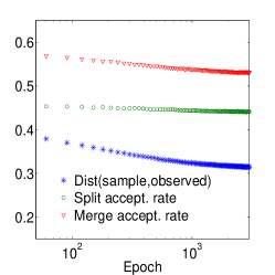
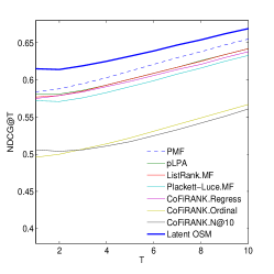
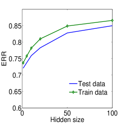
(a)	(b)	(c)

Figure 3: Results with MovieLens data. (a) Learning progress with time: Dist(sample,observed) is the portion of pairwise orders being incorrectly sampled by the split-and-merge Markov chains ($N=10$,$K=20$). (b) Rank completion, as measured in NDCG@T ($N=20,\,K=50$). (c) Rank reconstruction ($N=10$) - trained on $9,000$ users and tested on $1,000$ users.

We evaluate our proposed model and inference on large-scale collaborative filtering datasets: the MovieLens $10$M and the Netflix challenge. The MovieLens dataset consists of slightly over $10$ million half-integer ratings (from $0$ to $5$) applied to $10,681$ movies by $71,567$ users. The ratings are from $0.5$ to $5$ with $0.5$ increments. We divide the rating range into $5$ segments of equal length., and those ratings from the same segment will share the same rank. The Netflix dataset has slightly over $100$ million ratings applied to $17,770$ movies by $480,189$ users, where ratings are integers in a $5$-star ordinal scale.

Data likelihood estimation. Table 1 shows the log-likelihood of test data averaged over $100$ users with different numbers of movies per user. Results for the Latent OSM are estimated using the AIS procedure.

	$M=10$	$M=20$	$M=30$
Plackett-Luce.MF	-14.7	-41.3	-72.6
Latent OSM	-9.8	-37.9	-73.4

Table 1: Average log-likelihood over $100$ users of test data (Movie Lens $10$M dataset), after training on the $N=10$ movies per user ($K=10$). $M$ is the number of test movies per user. The Plackett-Luce.MF and the Latent OSM are comparable because they are both probabilistic in ranks and can capture latent aspects of the data. The main difference is that the Plackett-Luce.MF does not handle groupings or ties.

Rank reconstruction. Given the posterior vector, we ask whether we can reconstruct the original rank of movies for that data instance. For simplicity, we only wish to obtain a complete ranking, since it is very efficient (e.g. a typical cost would be $N\log N$ per user). Figure 3(c) indicates that high quality rank reconstruction (on both training and test data) is possible given enough hidden units. This suggests an interesting way to store and process rank data by using vectorial representation.

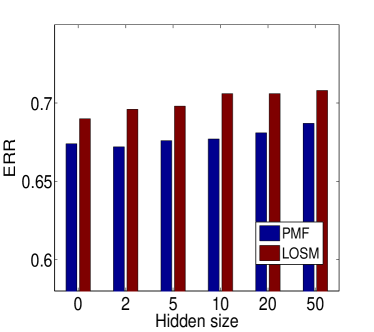
(a) MovieLens, $N=20$		(b) Netflix $N=10$

Figure 4: Rank completion quality vs. number of hidden units - note that since the PMF is not defined when hidden size is $0$, we substitute using the result for hidden size $1$.

Rank completion. In collaborative filtering settings, we are interested in ranking unseen movies for a given user. To highlight the disparity between user tastes, we remove movies whose qualities are inherently good or bad, that is when there is a general agreement among users. More specifically, we compute the movie entropy as $H_{i}=-\sum_{r=1}^{5}P_{i}(r)\log P_{i}(r)$ where $P_{i}(r)$ is estimated as the proportion of users who rate the movie $i$ by $r$ points. We then remove half of the movies with lowest entropy. For each dataset, we split the data into a training set and a test set as follows. For each user, we randomly choose $10$, $20$ and $50$ items for training, and the rest for testing. To ensure that each user has at least $10$ test items, we keep only those users with no less than $20$, $30$ and $60$ ratings, respectively.

Figs. 3(b), 4(a) and Table 2 report the results on the MovieLens $10$M dataset; Figs. 4(b) and Table 3 show the results for the Netflix dataset. It can be seen that the Latent OSM performs better than rivals when $N$ is moderate. For large $N$, the rating-based method (PMF) seems to work better, possibly because converting rating into ordering loses too much information in this case, and it is more difficult for the Latent OSM to explore the hyper-exponential state-space .

	$N=10$		$N=20$		$N=50$
	ERR	N@5	ERR	N@5	ERR	N@5
PMF	0.673	0.603	0.687	0.612	0.717	0.638
pLPA	0.674	0.596	0.684	0.601	0.683	0.595
ListRank.MF	0.683	0.603	0.682	0.601	0.684	0.595
Plackett-Luce.MF	0.663	0.586	0.677	0.591	0.681	0.586
CoFiRANK.Regress	0.675	0.597	0.681	0.598	0.667	0.572
CoFiRANK.Ordinal	0.623	0.530	0.621	0.522	0.622	0.515
CoFiRANK.N@10	0.615	0.522	0.623	0.517	0.602	0.491
Latent OSM	0.690	0.619	0.708	0.632	0.710	0.629

Table 2: Model comparison on the MovieLens data for rank completion ($K=50$). N@$T$ is a shorthand for NDCG@$T$.

	$N=10$				$N=20$
	ERR	N@1	N@5	N@10	ERR	N@1	N@5	N@10
PMF	0.678	0.586	0.607	0.649	0.691	0.601	0.624	0.661
ListRank.MF	0.656	0.553	0.579	0.623	0.658	0.553	0.577	0.617
Latent OSM	0.694	0.611	0.628	0.666	0.714	0.638	0.648	0.680

Table 3: Model comparison on the Netflix data for rank completion ($K=50$).

5 Related Work

This work is closely related to the emerging concept of preferences over sets in AI [3, 22] and in social choice and utility theories [1]. However, most existing work has focused on representing preferences and computing the optimal set under preference constraints [2]. These differ from our goals to model a distribution over all possible set orderings and to learn from example orderings. Learning from expressed preferences has been studied intensively in AI and machine learning, but they are often limited to pairwise preferences or complete ordering [5, 23].

On the other hand, there has been very little work on learning from ordered sets [26, 22]. The most recent and closest to our is the PMOP which models ordered sets as a locally normalised high-order Markov chain [19]. This contrasts with our setting which involves a globally normalised log-linear solution. Note that since the high-order Markov chain involves all previously ranked subsets, while our OSM involves pairwise comparisons, the former is not a special case of ours. Our additional contribution is that we model the space of partitioning and ordering directly and offer sampling tools to explore the space. This ease of inference is not readily available for the PMOP. Finally, our solution easily leads to the introduction of latent variables, while their approach lacks that capacity.

Our split-and-merge sampling procedure bears some similarity to the one proposed in [8] for mixture assignment. The main difference is that we need to handle the extra orderings between partitions, while it is assumed to be exchangeable in [8]. This causes a subtle difference in generating proposal moves. Likewise, a similar method is employed in [14] for mapping a set of observations into a set of landmarks, but again, ranking is not considered.

With respect to collaborative ranking, there has been work focusing on producing a set of items instead of just ranking individual ones [13]. These can be considered as a special case of OSM where there are only two subsets (those selected and the rest).

6 Conclusion and Future Work

We have introduced a latent variable approach to modelling ranked groups. Our main contribution is an efficient split-and-merge MCMC inference procedure that can effectively explore the hyper-exponential state-space. We demonstrate how the proposed model can be useful in collaborative filtering. The empirical results suggest that proposed model is competitive against state-of-the-art rivals on a number of large-scale collaborative filtering datasets.

References

- [1] S. Barberà, W. Bossert, and P.K. Pattanaik. Ranking sets of objects. Handbook of Utility Theory: Extensions, 2:893, 2004.
- [2] M. Binshtok, R.I. Brafman, S.E. Shimony, A. Martin, and C. Boutilier. Computing optimal subsets. In Proceedings of the National Conference on Artificial Intelligence, volume 22, page 1231. Menlo Park, CA; Cambridge, MA; London; AAAI Press; MIT Press; 1999, 2007.
- [3] R.I. Brafman, C. Domshlak, S.E. Shimony, and Y. Silver. Preferences over sets. In Proceedings of the National Conference on Artificial Intelligence, volume 21, page 1101. Menlo Park, CA; Cambridge, MA; London; AAAI Press; MIT Press; 1999, 2006.
- [4] O. Chapelle, D. Metlzer, Y. Zhang, and P. Grinspan. Expected reciprocal rank for graded relevance. In CIKM, pages 621–630. ACM, 2009.
- [5] W.W. Cohen, R.E. Schapire, and Y. Singer. Learning to order things. J Artif Intell Res, 10:243–270, 1999.
- [6] R.R. Davidson. On extending the Bradley-Terry model to accommodate ties in paired comparison experiments. Journal of the American Statistical Association, 65(329):317–328, 1970.
- [7] O. Dekel, C. Manning, and Y. Singer. Log-linear models for label ranking. Advances in Neural Information Processing Systems, 16, 2003.
- [8] S. Jain and R.M. Neal. A split-merge Markov chain Monte Carlo procedure for the Dirichlet process mixture model. Journal of Computational and Graphical Statistics, 13(1):158–182, 2004.
- [9] K. Järvelin and J. Kekäläinen. Cumulated gain-based evaluation of IR techniques. ACM Transactions on Information Systems (TOIS), 20(4):446, 2002.
- [10] N.N. Liu, M. Zhao, and Q. Yang. Probabilistic latent preference analysis for collaborative filtering. In CIKM, pages 759–766. ACM, 2009.
- [11] M. Mureşan. A concrete approach to classical analysis. Springer Verlag, 2008.
- [12] R.M. Neal. Annealed importance sampling. Statistics and Computing, 11(2):125–139, 2001.
- [13] R. Price and P.R. Messinger. Optimal recommendation sets: Covering uncertainty over user preferences. In Proceedings of the National Conference on Artificial Intelligence, volume 20, page 541. Menlo Park, CA; Cambridge, MA; London; AAAI Press; MIT Press; 1999, 2005.
- [14] A. Ranganathan, E. Menegatti, and F. Dellaert. Bayesian inference in the space of topological maps. Robotics, IEEE Transactions on, 22(1):92–107, 2006.
- [15] R. Salakhutdinov and A. Mnih. Probabilistic matrix factorization. Advances in neural information processing systems, 20:1257–1264, 2008.
- [16] R. Salakhutdinov and I. Murray. On the quantitative analysis of deep belief networks. In Proceedings of the 25th international conference on Machine learning, pages 872–879. ACM, 2008.
- [17] Y. Shi, M. Larson, and A. Hanjalic. List-wise learning to rank with matrix factorization for collaborative filtering. In ACM RecSys, pages 269–272. ACM, 2010.
- [18] P. Smolensky. Information processing in dynamical systems: Foundations of harmony theory. Parallel distributed processing: Explorations in the microstructure of cognition, 1:194–281, 1986.
- [19] T. Truyen, D.Q Phung, and S. Venkatesh. Probabilistic models over ordered partitions with applications in document ranking and collaborative filtering. In Proc. of SIAM Conference on Data Mining (SDM), Mesa, Arizona, USA, 2011. SIAM.
- [20] J.H. van Lint and R.M. Wilson. A course in combinatorics. Cambridge Univ Pr, 1992.
- [21] S. Vembu and T. Gärtner. Label ranking algorithms: A survey. Preference Learning, page 45, 2010.
- [22] K.L. Wagstaff, Marie desJardins, and E. Eaton. Modelling and learning user preferences over sets. Journal of Experimental & Theoretical Artificial Intelligence, 22(3):237–268, 2010.
- [23] M. Weimer, A. Karatzoglou, Q. Le, and A. Smola. CoFiRANK-maximum margin matrix factorization for collaborative ranking. Advances in neural information processing systems, 20:1593–1600, 2008.
- [24] M. Welling, M. Rosen-Zvi, and G. Hinton. Exponential family harmoniums with an application to information retrieval. In Advances in NIPS, volume 17, pages 1481–1488. 2005.
- [25] L. Younes. Parametric inference for imperfectly observed Gibbsian fields. Probability Theory and Related Fields, 82(4):625–645, 1989.
- [26] Y. Yue and T. Joachims. Predicting diverse subsets using structural SVMs. In Proceedings of the 25th international conference on Machine learning, pages 1224–1231. ACM, 2008.