Passive mode-locking under higher order effects

Abstract

The response of a passive mode-locking mechanism, where gain and spectral filtering are saturated with the energy and loss saturated with the power, is examined under the presence of higher order effects. These include third order dispersion, self-steepening and Raman gain. The locking mechanism is maintained even with these terms; mode-locking occurs for both the anomalous and normal regimes. In the anomalous regime, these perturbations are found to affect the speed but not the structure of the (locked) pulses. In fact, these pulses behave like solitons of a classical nonlinear Schrödinger equation and as such a soliton perturbation theory is used to verify the numerical observations. In the normal regime, the effect of the perturbations is small, in line with recent experimental observations. The results in the normal regime are verified mathematically using a WKB type asymptotic theory. Finally, bi-solitons are found to behave as dark solitons on top of a stable background and are significantly affected by these perturbations.

I Introduction

Ultrashort pulses are used frequently in modern applications ranging from femtochemistry and medical imaging to micro-machining and optical communications. Consequently the study and modeling of such pulses is an important area of research. Kerr-lens mode locking (KLM) is a common technique used to generate these pulses. In fact, following the discovery of KLM mode-locked (ML) lasers have revolutionized the field of ultrafast science and their performance has led to their widespread use.

Mode-locked lasers operate under the requirement that sufficient amounts of gain and loss are present, otherwise, they are subject to radiation-mode instability. In addition, passive mode-locking generally utilizes fast saturable absorbers which are effectively simulated by KLM. Saturable absorbers are commonly modeled by a transfer function and as such loss is placed periodically during the evolution and not as part of a distributed model, i.e., an evolution equation. However, the qualitative features are the same in both cases horikis2 thus indicating that distributive models are very good descriptions of modes in mode-locked lasers.

Modeling these lasers must take into account their physical properties. For this, the distributive power-energy saturation (PES) model was recently introduced horikis5 . This system is a variant of the well known nonlinear Schrödinger (NLS) equation with additional terms to account for gain and spectral filtering, saturated with energy, and loss, saturated with power. It is a generalization of the commonly used master-equation master1 ; master3 which is obtained as a limiting case. Mode-locking is much more robust in the PES model than in the master-equation. Indeed, while in the master-equation mode-locking is achieved only for a narrow range of parameters kutz ; kutz2 , the PES equation has only one key requirement for mode-locking: sufficient gain. Another important feature of the PES equation is that it leads to physically relevant results for both the anomalous and normal dispersive regimes.

Solitons in ML lasers are fundamentally different in the two dispersive regimes. Pulse formation, in the anomalous regime, is typically dominated by the interplay between dispersion and nonlinearity. Suitable gain media and an effective saturable absorber are required for initiation of pulsed operation. In contrast, pulses found in the normal regime are positively chirped throughout the cavity ilday . They are comprised of an approximately parabolic temporal amplitude profile near the peak of the pulse with a transition to steep decay ilday . Pulses in the normal regime have a much larger temporal width than those in the anomalous regime.

Here we study the response of a ML laser under higher order effects using the PES equation. These effects include third-order dispersion (TOD), self-steepening and Raman gain. Previous studies, in the anomalous dispersion regime, include variants of the master-equation haus ; lin and generalized Ginzburg-Landau type equations kalashnikov ; song ; sorokin . In the normal regime recent experiments oktem indicate that similariton (self-similar) evolution in these fiber lasers results in localized modes, i.e. solitons, which are broad in the time domain; they are robust against perturbations. The effect of TOD on self-similar evolution and parabolic pulses was studied in Refs. dudley ; bale ; zhang .

Here we focus on the equation

$$i\frac{{\partial u}}{{\partial z}}+\frac{{{d_{0}}}}{2}\frac{{{\partial^{2}}u}}{{\partial{t^{2}}}}+|u{|^{2}}u =\frac{{igu}}{{1+\epsilon E}}+\frac{{i\tau}}{{1+\epsilon E}}\frac{{{\partial^{2}}u}}{{\partial{t^{2}}}}-\frac{{ilu}}{{1+\delta P}}$$

$$+i\beta\frac{{{\partial^{3}}u}}{{\partial{t^{3}}}}-i\gamma\frac{\partial(|u|^{2}u)}{\partial t}+Ru\frac{{\partial(|u|^{2})}}{{\partial t}}$$ (1)

where $g$ represents gain saturated with the energy $E=\int_{-\infty}^{\infty}|u|^{2}\;dt$, $\tau$ is spectral filtering, $l$ is the gain saturated with power $P=|u|^{2}$, $\beta$ represents TOD, $\gamma$ self-steepening and $R$ the Raman gain. The parameters $\epsilon>0$ and $\delta>0$ correspond to a measure of the saturation energy and power of the system, respectively. Unless otherwise stated all parameters, except $d_{0}$, are positive. When $\beta=\gamma=R=0$ this equation is the PES model. Finally, other linear and higher order nonlinear dissipative terms, such as terms proportional to $iu$ and $i|u|^{2}u$ are included in Eq. (1) as limiting cases in the expansion for the saturable terms and will not be considered here.

II The anomalous dispersion regime

Here we consider Eq. (1) with $d_{0}>1$ and we start our analysis by analyzing the effect of TOD. To do so, we fix the parameters such that $\tau=l=0.1$, $d_{0}=\epsilon=\delta=1$ and $\beta=0.01$ while $\gamma=R=0$ and vary the gain parameter $g$. A unit gaussian is evolved under Eq. (1) with the resulting evolution shown in Fig. 1.

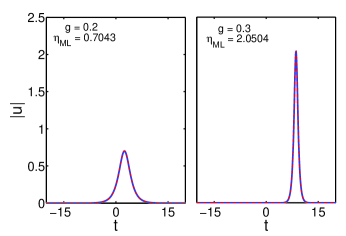
Figure 1: (Color online) Mode-locking under TOD with (a) $g=0.2$ and (b) $g=0.3$. The bottom figures show the pulse at a distance $z=150$ (a sufficient distance of propagation after mode-locking has occurred). The dashed lines correspond to the relative classical NLS solitons.

As seen here, the initial gaussian undergoes a locking procedure and subsequently locks to a pulse of constant height/shape. After that happens the effect of TOD shifts the soliton with constant velocity (seen as a straight line for the soliton center in the top of Fig. 1). Interestingly the resulting mode is a solution of the unperturbed NLS equation. Furthermore, when the gain is increased the angle of the displacement becomes more acute. This is reminiscent of the response of a single soliton of the classical NLS equation to TOD. Indeed, recall that under TOD the NLS soliton is slowed down and as a result the soliton peak is shifted by an amount that increases linearly with distance book2 ; book1 .

Similarly, we repeat the analysis for $\beta=R=0$ and $\gamma=0.01$ so as to study the response to self-steepening. The resulting evolution is depicted in Fig. 2.

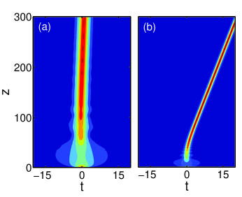
Figure 2: (Color online) Mode-locking under self-steepening with (a) $g=0.2$ and (b) $g=0.3$. Profiles of mode-locked pulses resemble those of Fig. 1 (bottom).

The similarities between Figs. 1 and 2 are remarkable. Indeed, after mode-locking occurs the pulse is shifted linearly in a way that is similar to the way a classical NLS soliton propagates under this effect.

Finally, we repeat the analysis for $\beta=\gamma=0$ and $R=0.01$ so as to study the response to the Raman gain. The resulting evolution is depicted in Fig. 3.

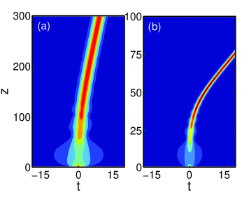
Figure 3: (Color online) Mode-locking under Raman gain with (a) $g=0.2$ and (b) $g=0.3$. Profiles of mode-locked pulses resemble those of Fig. 1 (bottom).

The phenomenon is repeated only now the displacement is sharper. Again, recall that Raman gain on solitons of the classical NLS equation gives rise to the so-called self-frequency shift book2 ; book1 . Note the size of the pulse amplitude is largely unaffected.

It is also important to stress that this locking behavior strongly depends on the saturation terms. If these terms/effects are absent more complicated dynamics can occur sorokin .

II.1 Perturbation theory

Now we shall explain the above features using soliton perturbation theory valid for small $\beta$, $\gamma$, $R$. This approach leads to very good qualitative results since when $\beta=\gamma=R=0$ general initial conditions, such as unit gaussians, will evolve to solitons of the unperturbed classical NLS equation horikis7 . To do this, we consider a solution ansatz for Eq. (1) of the form

$$u(z,t)=\eta(z)\mathrm{sech}[\eta(z)(t-t_{0}(z))]e^{i\phi(z)-i\sigma(z)t}$$

Under the effect of the perturbed PES the soliton parameters evolve according to horikis1 ; book1 ; book2

$$\frac{{d\eta}}{{dz}} =\frac{{2g\eta}}{{1+2\epsilon\eta}}-\frac{{2\tau({\eta^{2}}+3{\sigma^{2}})}}{{3(1+2\epsilon\eta)}}\eta-\frac{{2l{{\tanh}^{-1}}\left({\frac{{\sqrt{\delta}\eta}}{{\sqrt{1+\delta{\eta^{2}}}}}}\right)}}{{\sqrt{\delta+{\delta^{2}}{\eta^{2}}}}}$$ (2a)

$$\frac{{d\sigma}}{{dz}} =-\frac{{4\tau{\eta^{2}}\sigma}}{{3(1+2\epsilon\eta)}}-\frac{8}{{15}}R{\eta^{4}}$$ (2b)

$$\frac{{d{t_{0}}}}{{dz}} =-\sigma+\beta(\eta^{2}+3\sigma^{2})+\gamma\eta^{2}$$ (2c)

$$\frac{{d\phi}}{{dz}} =\beta\sigma(3{\eta^{2}}+{\sigma^{2}})+\gamma\eta^{2}+\frac{1}{2}({\eta^{2}}-{\sigma^{2}})+{t_{0}}\frac{{d\sigma}}{{dz}}$$ (2d)

When the pulse has mode-locked, the zeroes of the right hand side of Eq. (2a)-(2b) give the stationary solutions for $\eta$ and $\sigma$. We denote the mode locked value of $\eta$ and $\sigma$ as $\eta_{ML}$ and $\sigma_{ML}$, respectively. As such when the equilibrium has been reached

$$\sigma\equiv\sigma_{ML}=-\frac{2R(1+2\epsilon\eta)\eta^{2}}{5\tau}$$

this results in the following equation for $\eta$

$$\frac{d\eta}{dz}=\frac{{2g\eta}}{{1+2\epsilon\eta}} -\frac{2\left[25\tau^{2}\eta^{2}+12(2\epsilon R\eta+R)^{2}\eta^{4}\right]}{75(\tau+2\epsilon\tau\eta)}$$

$$-\frac{{2l{{\tanh}^{-1}}\left({\frac{{\sqrt{\delta}\eta}}{{\sqrt{1+\delta{\eta^{2}}}}}}\right)}}{{\sqrt{\delta+{\delta^{2}}{\eta^{2}}}}}$$

Clearly, $\eta$ has at least one equilibrium at $\eta=0$. To understand its stability consider the first derivative of $\eta_{z}$ with respect to $\eta$ evaluated at $\eta=0$,

$$\left.\frac{d}{d\eta}\left(\frac{d\eta}{dz}\right)\right|_{\eta=0}=2(g-l)$$

When $g>l,\eta=0$ is an unstable equilibrium while for $g<l,\eta=0$ is stable. The phase portrait for various values of $g<l$ indicates that $\eta_{z}$ is a monotonic decreasing function in $\eta$ and so $\eta\rightarrow 0$ as $z\rightarrow\infty$ for any initial condition $\eta>0$. Physically this corresponds to loss overtaking gain and the pulse decays. For $g>l$, $\eta_{z}$ is initially positive and as $\eta$ increases the filtering term becomes dominant and $\eta_{z}$ takes on negative values. Thus, there must exist another equilibrium. Plotting the phase portrait for various values of $g$ for $g>l$ shows there is a single stable equilibrium for $\eta>0$, as shown in Fig. 4.

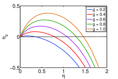
Figure 4: Phase portrait of the amplitude equation for several values of $g$ illustrating the single stable equilibrium. Here $l=0.1$.

As $\eta$ approaches its stable equilibrium, $\eta_{ML}\neq 0$, and $\sigma$ approaches its stable equilibrium, $\sigma_{ML}$, the system of equations (2) tend to

$$\left.\frac{d\eta}{dz}\right|_{\eta=\eta_{ML}}=\left.\frac{d\sigma}{dz}\right|_{\sigma=\sigma_{ML}}=0$$

which means the solition tends to a particular NLS soliton of speed zero and height/width determined by $\eta_{ML}$, thus suggesting the mode-locking capabilities of Eq. (1). In fact, $\eta_{ML}$ is an attractor that any arbitrary initial condition will eventually converge to, even when it is far way from its soliton solution horikis5 ; horikis7 .

After $\eta=\eta_{ML}$ and mode-locking has been completed, we consider Eq. (2c)-(2d), which, interestingly, are independent of $g,\tau,l$. This now explains the above dynamics. Indeed, when $\eta=\eta_{ML}$ (and the mode-locking mechanism has been completed) we get by direct integration of Eq. (2c)

$$t_{0}(z) =t_{0}(0)+\left\{\left(\beta+\gamma+\frac{2R}{5\tau}\right)\eta_{ML}^{2}\right.$$

$$\left.+\frac{4R\left[3\beta R(2\epsilon\eta_{ML}+1)^{2}\eta_{ML}+5\epsilon\tau\right]\eta_{ML}^{3}}{25\tau^{2}}\right\}z$$ (3)

The equations for the equilibria give now more insight as to the way each term affects the propagation. For instance, in the absence of spectral filtering there still exists a stable (nonzero) equilibrium for $\eta$ but not for $\sigma$. While the amplitude is affected only in its magnitude the other quantities change in a more prominent way. Indeed, by direct integration of Eqs. (2b) and (2c) we obtain at $\eta=\eta_{ML}$

$$\sigma(z) =-\frac{8}{{15}}R{\eta_{ML}^{4}}z+\sigma(0)$$

$$t_{0}(z) =\frac{64}{225}R^{2}\beta\eta_{ML}^{8}z^{3}-\frac{4}{15}R\eta_{ML}^{4}[6\beta\sigma(0)-1]z^{2}$$

$$+[(\beta+\gamma)\eta_{ML}^{2}+3\beta\sigma^{2}(0)-3\sigma(0)]z+t_{0}(0)$$

which suggests that the trajectory the soliton follows is no longer linear. Similarly when the Raman gain is not considered the only equilibrium is found for $\sigma\equiv 0$. Clearly when $\tau=R=0$ the soliton moves with constant velocity equal to $(\beta+\gamma)\eta_{ML}^{2}$ ($\sigma\equiv 0$). Also, note that as supported by the numerical computations the final amplitude of the pulse is not affected by the parameters $\beta,\gamma$.

The increase of $\eta$ with $g$ also explains the pronounced difference in the speed of the pulse when $g$ is increased. In Fig. 5 we depict the dependance of the amplitude to the gain parameter, which attests to that.

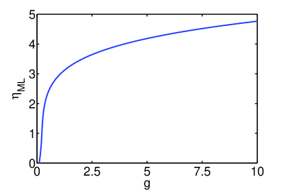
Figure 5: (Color online) The amplitude dependance on gain based on Eq. (2a).

In fact, Eq. (3) clearly suggests that the trajectories are highly dependent on powers of $\eta_{ML}$. Hence, any increase on this amplitude is enhanced (when $\eta_{ML}>1$ or $g>0.22$) making the response to the perturbations more pronounced. This analysis also suggests that nonlinear phase shifts cannot compensate for TOD (or self-steepening) in this regime, unlike in the normal regime zhou .

Thus, the mode-locking mechanism can now be summarized as follows: (i) solve Eqs. (2a)-(2b), to determine $\eta_{ML}$ and $\sigma_{ML}$; (ii) assume the mode-locking mechanism has been completed; (iii) treat the pulses as classical NLS solitons; and (iv) use Eq. (3) and (2d) to determine the adiabatic change of the rest of the soliton parameters.

III The normal dispersion regime

We turn our attention to the normal regime ($d_{0}=-1$). The main difference these pulses exhibit from their anomalous regime counterparts is that they are highly chirped, very wide (almost parabolic) pulses in the time domain; the modes depend critically on the values of $g,\tau,l$.

Recent experiments indicate that localized modes– solitons in the normal regime are robust. They are not affected by perturbations oktem such as TOD and self steepening; this is also in agreement with the observation that nonlinear phase shifts (in terms of Raman gain here) can compensate for TOD or self-steepening zhou . To demonstrate this phenomena, we evolve a unit gaussian under Eq. (1), with all parameters as before ($\tau=l=0.1$, $\beta=\gamma=R=0.01$) only now with $g=1.5$. The reason for this increase in gain is the nature/size of these pulses (cf. Fig. 6).

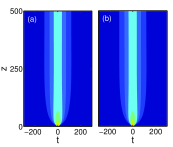
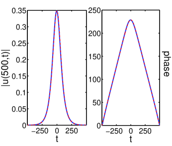
Figure 6: (Color online) Mode-locking in the normal regime (a) under the unperturbed PES equation with $\beta=\gamma=R=0$ and (b) under the PES with the higher order effects included. The bottom figure depicts the final pulse. The dashed line is the soliton of the unperturbed PES equation.

Since these pulses are much wider one expects that more energy (gain) is required for pulses to lock to noticeable amplitudes. Furthermore, in Fig. 6 (bottom) we depict the resulting pulse and its corresponding phase. The dashed line indicates the soliton of the unperturbed (i.e. $\beta=\gamma=R=0$) PES equation. Indeed the experimental observations ilday on the shape and phase of the pulses are met. We also confirm subsequent observations that unlike the solitons of the anomalous regime these wide localized pulses are resistant to perturbations even when allowed to propagate for greater distances.

III.1 Asymptotic theory

Following the theory developed in Ref. horikis4 we write the solution of Eq. (1) in the form $\psi(z,t)=A\exp(i\mu z+i\theta)$, where $A=A(t)$ and $\theta=\theta(t)$ are the pulse amplitude and phase respectively. Since these pulses are slowly varying in $t$, with large phase, we can introduce a slow time scale in the equation and using perturbation theory, the soliton system can be reduced to simpler ordinary differential equations for the amplitude and the phase of the pulse. Substituting into the equation and equating real and imaginary parts we get

$$-\mu A-\frac{{{d_{0}}}}{2}({A_{tt}}-A\theta_{t}^{2})+{A^{3}}=-\frac{\tau}{{1+\epsilon E}}(2{A_{t}}{\theta_{t}}+A{\theta_{tt}})$$

$$+\beta(A{\theta_{tt}}-3{A_{tt}}{\theta_{t}}-3{A_{t}}{\theta_{tt}}-A{\theta_{ttt}})+\gamma{A^{3}}{\theta_{t}}+2R{A^{2}}{A_{t}}$$ (4a)

$$-\frac{{{d_{0}}}}{2}(2{A_{t}}{\theta_{t}}+A{\theta_{tt}})=\frac{g}{{1+\epsilon E}}A+\frac{\tau}{{1+\epsilon E}}({A_{tt}}+A\theta_{t}^{2})$$

$$-\frac{l}{{1+\delta{A^{2}}}}A+\beta(3{A_{t}}\theta_{t}^{2}-3A{\theta_{t}}{\theta_{tt}}+{A_{ttt}})-3\gamma{A^{2}}{A_{t}}$$ (4b)

where we have replaced $d_{0}\rightarrow-d_{0}<0$ since we are in the normal dispersion regime. We then take the characteristic time length of the pulse to be such that we can define a scaling in the independent variable of the form $\varepsilon=T/\varepsilon$ or $T=\varepsilon t$ so that $R=R(\varepsilon t)$, $\theta_{t}=O(1)$ (i.e. $\theta$ is large) and $\theta_{tt}=O(\varepsilon)$ where $\varepsilon\ll 1$. Furthermore in the above simulations $\beta$, $\gamma$ and $R$ are all $O(\varepsilon)$. Then Eq. (4a) becomes

$$-\mu A+\frac{d_{0}}{2}A\theta_{t}^{2}+A^{3}=\frac{d_{0}}{2}\varepsilon^{2}A_{TT}-\frac{\tau}{1+\epsilon E}(2\varepsilon A_{T}\theta_{t}+A\theta_{tt})$$

while the leading order equation is

$$\theta_{t}^{2}=\frac{2}{d_{0}}(\mu-A^{2})$$ (5)

Using the same argument and this newly derived Eq. (5) we then find that Eq. (4b) to leading order reads

$$A_{t}= -\mathrm{sgn}(t)\frac{\sqrt{2(\mu-A^{2})/d_{0}}}{3A^{2}-2\mu}$$

$$\times\left(\frac{g}{1+\epsilon E}-\frac{4\tau(\mu-A^{2})/d_{0}}{1+\epsilon E}-\frac{l}{1+\delta A^{2}}\right)$$ (6)

This is now a nonlocal first order differential equation for $A=A(t)$, since $E=\int_{-\infty}^{\infty}A^{2}\;dt$. We also note that imposing $\theta_{t}(t=0)=0\Rightarrow\mu\approx A^{2}(0)$.

To remove the nonlocality another condition is needed and it is based on the singular points of Eq. (6). Recall, $A(t)$ is a decaying function in $t\in[0,+\infty)$ and $\mu\approx A^{2}(0)\geq A(t)^{2}$. Thus there exists a point in $t$ such that the denominator in the equation becomes zero. To remove the singularity we require that the numerator of the equation is also zero at the same point which leads to

$$1+\epsilon E=\frac{1}{l}\left(g-\frac{2\tau}{3d_{0}}\mu\right)\left(1+\frac{2\delta}{3}\mu\right)$$

Thus Eq. (6) is now a first order equation which can be solved by standard numerical methods and analyzed by phase plane methods. The resulting solutions from the PES equation and the reduced equations are compared in Fig. 7.

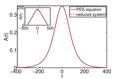
Figure 7: (Color online) Solutions of the complete PES equation and the reduced system.

III.2 Higher order states

Remarkably, in the normal regime the PES also exhibits higher-order solutions in term of bi-solitons chong . These are pairs of regular solitons whose peak amplitudes have a $\pi$ difference in phase and an appropriate separation. They, also, differ significantly from the higher-order solutions of the classical NLS and the dispersion managed solitons since they do not exhibit any oscillatory or breathing behavior as they propagate in the cavity. A typical such mode is given in Fig. 8. The dashed line corresponds to the relative “ground state”, i.e. the localized pulse of the unperturbed PES equation.

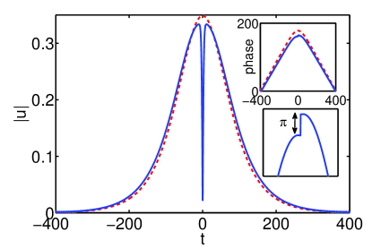
Figure 8: (Color online) A typical bisoliton of the PES. Dashed lines correspond to the soliton and phase of the localized pulse of the unperturbed PES equation.

Higher order states and interaction of these structures have been discussed in Ref. horikis6 . It is, however, interesting to see their response to TOD and Raman gain. In order to generate these modes we use an antisymmetric initial condition such as $u(0,t)=t\exp(-t^{2})$. The resulting evolution, under Eq. (1), is shown in Fig. 9.

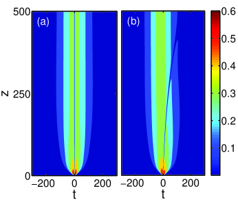
Figure 9: (Color online) Bisoliton evolution (a) under the PES equation; (b) under Eq. (1).

Under these higher order effects the dip characterizing the bi-soliton, which separates the two solitons, behaves as a dark soliton on a nearly constant background and starts moving until it disappears; see Fig. 9. This is reminiscent of the dark solitons generated in Bose-Einstein condensates dfrantz . We will further explore this elsewhere.

IV Conclusions

To conclude, we have studied the response of a PES model with additional higher order terms: third order dispersion, self-steepening and Raman gain. In the anomalous dispersion regime, it is found that the PES equation provides the mode-locking mechanism and after that the resulting pulses propagate in a manner similar to solitons of a perturbed classical NLS equation. Perturbative soliton theory confirms numerical observations. On the other hand, in the normal dispersion regime, ground state pulses are more robust and are largely unaffected by these perturbing influences as also observed in experiments. However, this is not the case with higher order modes which are unstable when perturbed.

- (1) M. J. Ablowitz and T. P. Horikis, “Solitons and spectral renormalization methods in nonlinear optics,” Eur. Phys. J. Special Topics 173, 147–166 (2009).
- (2) M. J. Ablowitz, T. P. Horikis, and B. Ilan, “Solitons in dispersion-managed mode-locked lasers,” Phys. Rev. A 77, 033814 (2008).
- (3) H. A. Haus, “Theory of mode locking with a fast saturable absorber,” J. Appl. Plys. 46, 3049–3058 (1975).
- (4) H. A. Haus, J. G. Fujimoto, and E. P. Ippen, “Analytic theory of additive pulse and kerr lens mode locking,” IEEE J. Quant. Elec. 28, 2086–2096 (1992).
- (5) J. N. Kutz, “Mode-locked soliton lasers,” SIAM Rev. 48, 629–678 (2006).
- (6) T. Kapitula, J. N. Kutz, and B. Sandstede, “Stability of pulses in the master mode-locking equation,” J. Opt. Soc. Am. B 19, 740–746 (2002).
- (7) F. O. Ilday, J. R. Buckley, W. G. Clark, and F. W. Wise, “Self-similar evolution of parabolic pulses in a laser,” Phys. Rev. Lett. 92, 213901 (2004).
- (8) H. A. Haus, J. D. Moores, and L. E. Nelson, “Effect of third-order dispersion on passive mode locking,” Opt. Lett. 18, 51–53 (1993).
- (9) Q. Lin and I. Sorokina, “High-order dispersion effects in solitary mode-locked lasers: side-band generation,” Opt. Commun. 153, 285–288 (1998).
- (10) V. L. Kalashnikov, A. Fernández, and A. Apolonski, “High-order dispersion in chirped-pulse oscillators,” Opt. Express 16, 4206–4216 (2008).
- (11) L. Song, L. Li, Z. Li, and G. Zhou, “Effect of third-order dispersion on pulsating, erupting and creeping solitons,” Opt. Commun. 249, 301–309 (2005).
- (12) E. Sorokin, N. Tolstik, V. L. Kalashnikov, and I. T. Sorokina, “Chaotic chirped-pulse oscillators,” Opt. Express 21, 29567–29577 (2013).
- (13) B. Oktem, C. Ülgüdür, and F. O. Ilday, “Soliton-similariton fibre laser,” Nature Photonics 4, 307–311 (2010).
- (14) J. M. Dudley, C. Finot, D. J. Richardson, and G. Millot, “Self-similarity in ultrafast nonlinear optics,” Nature Physics 3, 597–603 (2007).
- (15) B. G. Bale and S. Boscolo, “Impact of third-order fibre dispersion on the evolution of parabolic optical pulses,” J. Opt. 12, 015202 (2010).
- (16) S. Zhang, G. Zhao, A. Luo, and Z. Zhang, “Third-order dispersion role on parabolic pulse propagation in dispersion-decreasing fiber with normal group-velocity dispersion,” Appl. Phys. B 94, 227–232 (2009).
- (17) A. Hasegawa and Y. Kodama, Solitons in Optical Communications (Claredo Press, 1995).
- (18) Y. S. Kivshar and G. P. Agrawal, Optical Solitons (Academic Press, 2003).
- (19) M. J. Ablowitz and T. P. Horikis, “Pulse dynamics and solitons in mode-locked lasers,” Phys. Rev. A 78, 011802(R) (2008).
- (20) M. J. Ablowitz, T. P. Horikis, S. D. Nixon, and Y. Zhu, “Asymptotic analysis of pulse dynamics in mode-locked lasers,” Stud. Appl. Math 122, 411–425 (2009).
- (21) S. Zhou, L. Kuznetsova, A. Chong, and F. W. Wise, “Compensation of nonlinear phase shifts with third-order dispersion in short-pulse fiber amplifiers,” Opt. Express 13, 4869–4877 (2005).
- (22) M. J. Ablowitz and T. P. Horikis, “Solitons in normally dispersive mode-locked lasers,” Phys. Rev. A 79, 063845 (2009).
- (23) A. Chong, W. H. Renninger, and F. W. Wise, “Observation of antisymmetric dispersion-managed solitons in a mode-locked laser,” Opt. Lett. 33, 1717–1719 (2008).
- (24) M. J. Ablowitz, T. P. Horikis, and S. D. Nixon, “Soliton strings and interactions in mode-locked lasers,” Opt. Comm. 282, 4127–4135 (2009).
- (25) D. J. Frantzeskakis, “Dark solitons in atomic bose-einstein condensates: from theory to experiments,” J. Phys. A: Math. Theor. 43, 213001 (2010).