High-Throughput Computational Screening of thermal conductivity, Debye temperature and Grüneisen parameter
using a quasi-harmonic Debye Model

Abstract

The quasi-harmonic Debye approximation has been implemented within the AFLOW and Materials Project frameworks for high-throughput computational materials science (Automatic Gibbs Library, AGL), in order to calculate thermal properties such as the Debye temperature and the thermal conductivity of materials. We demonstrate that the AGL method, which is significantly cheaper computationally compared to the fully ab initio approach, can reliably predict the ordinal ranking of the thermal conductivity for several different classes of semiconductor materials. In particular, a high Pearson (i.e. linear) correlation is obtained between the experimental and AGL computed values of the lattice thermal conductivity for a set of 75 compounds including materials with cubic, hexagonal, rhombohedral and tetragonal symmetry.

I Introduction

Calculating the thermal properties of materials is important for predicting the thermodynamic stability of structural phases and assessing their importance for a variety of applications. The lattice thermal conductivity, $\kappa_{l}$, is a crucial design parameter in a wide range of important technologies, such us the development of new thermoelectric materials zebarjadi_perspectives_2012 ; curtarolo:art84 , heat sink materials for thermal management in electronic devices Yeh_2002 , and rewritable density scanning-probe phase-change memories Wright_tnano_2011 . High thermal conductivity materials, which typically have a zincblende or diamond-like structure, are essential in microelectronic and nanoelectronic devices to achieve efficient heat removal Watari_MRS_2001 , and have been intensively studied for the past few decades Slack_1987 . Low thermal conductivity materials constitute the basis of a new generation of thermoelectric materials and thermal barrier coatings Snyder_jmatchem_2011 .

The determination of the thermal conductivity of materials is computationally demanding since it requires calculation of multiple-phonon scattering processes, that are the origin of the lattice resistance to heat transport. The methods most commonly used currently to calculate the thermal conductivity are based on solving the Boltzmann Transport Equation (BTE). This solution involves the calculation of the phonon frequencies, group velocities, and the harmonic and anharmonic interatomic force constants (IFCs) Broido2007 ; Wu_PRB_2012 . In particular, the third-order anharmonic IFCs are required in order to incorporate the effects of three phonon scattering processes Broido2007 ; Wu_PRB_2012 . The standard method to calculate these anharmonic IFCs is based on density functional theory (DFT). Deinzer et al. Deinzer_PRB_2003 used Density Functional Perturbation Theory (DFPT) to obtain third-order IFCs to study the phonon linewidths. In the last decade, this method has been successfully used to solve the BTE and predict the thermal conductivity of different materials Broido2007 ; ward_ab_2009 ; ward_intrinsic_2010 ; Wu_PRB_2012 ; Zhang_JACS_2012 ; Li_PRB_2012 ; Lindsay_PRL_2013 ; Lindsay_PRB_2013 . Such evaluation of the higher-order IFCs requires electronic structure calculations for multiple large supercells, each of which has a different set of atomic displacements. These first principles solutions of the BTE are therefore computationally extremely expensive.

A variety of simple methods have been devised to evaluate the thermal properties of materials at reduced computational cost. Early approximate implementations to compute the lattice thermal conductivity were based on semi-empirical models to solve the BTE, in which some parameters are obtained from fitting to experimental data ziman_electrons_2001 ; callaway_model_1959 ; Allen_PHMB_1994 . This reduces the predictive power of the calculations.

An alternative approach to calculating thermal conductivity is based on the Green-Kubo formula, which employs molecular dynamics simulations to calculate thermal currents over long time periods after thermal equilibrium is reached Green_JCP_1954 ; Kubo_JPSJ_1957 . This technique takes into account high order scattering processes, but the usage of semi-empirical potentials leads to errors on the order of 50$\%$ zebarjadi_perspectives_2012 .

The methods described above are unsuitable for rapid generation and screening of large databases of materials properties in order to identify trends and simple descriptors for thermal properties curtarolo:art81 . To accomplish this, we chose to implement a much cheaper approach, the “GIBBS” quasi-harmonic Debye model Blanco_CPC_GIBBS_2004 . This approach does not require large supercell calculations since it relies merely on first-principles calculations of the energy as a function of unit cell volume. It is thus much more tractable computationally and is eminently suited to investigating the thermal properties of entire classes of materials in a highly-automated fashion, in order to identify promising candidates for more in-depth experimental and computational analysis. We incorporate this model in a new software library, the Automatic GIBBS Library (AGL), within the AFLOW curtarolo:art65 ; aflowlibPAPER ; curtarolo:art92 and Materials Project materialsproject.org ; APL_Mater_Jain2013 ; CMS_Ong2012b frameworks for high-throughput computational materials science, and use it to construct a database of computed compound thermal conductivities and Debye temperatures.

II The Automatic GIBBS Library (AGL)

The AGL software library implements the “GIBBS” method Blanco_CPC_GIBBS_2004 in the AFLOW curtarolo:art65 ; aflowlibPAPER ; curtarolo:art92 framework (C++ based framework) and the Materials Project materialsproject.org ; APL_Mater_Jain2013 ; CMS_Ong2012b (Python implementation). The library includes automatic error handling and correction to facilitate high-throughput computation of materials thermal properties. The principal ingredients of the calculation are described in the following sections.

II.1 The GIBBS quasi-harmonic Debye model

In thermodynamics, the equilibrium state of a system at a constant temperature and pressure minimizes its Gibbs free energy

$$G(\vec{x};p,T)=E(\vec{x})+pV(\vec{x})+A_{vib}(\vec{x};T),$$ (1)

where $\vec{x}$ is a configuration vector containing all the information about the system’s geometry, $E(\vec{x})$ is the total energy of the crystal (obtained, for example, from an electronic structure calculation), $A_{vib}$ is the vibrational Helmholtz free energy, and $p$ and $V(\vec{x})$ are the pressure and volume. It is assumed here that the electronic and intrinsic point defect contributions to the Helmholtz free energy is small, which is a good approximation for most materials at temperatures significantly below their melting point. In the quasi-harmonic approximation, the Helmholtz vibrational energy is

$$A_{vib}(\vec{x};T)\!=\!\!\int_{0}^{\infty}\!\!\left[\frac{\hbar\omega}{2}\!+\!k_{B}T\ \mathrm{log}\!\left(1\!-\!{\mathrm{e}}^{-\hbar\omega/k_{B}T}\right)\!\right]\!g(\vec{x};\omega)d\omega,$$ (2)

where $g(\vec{x};\omega)$ is the phonon density of states. As mentioned before, calculation of the full phonon density of states is computationally demanding, requiring electronic structure calculations for multiple supercell configurations. Instead, the “GIBBS” method uses a quasi-harmonic Debye model, where the Helmholtz free energy is expressed in terms of the Debye temperature $\theta_{\mathrm{D}}$

$$A_{vib}(\theta_{D};T)\!=\!nk_{B}T\!\left[\frac{9}{8}\frac{\theta_{\mathrm{D}}}{T}\!+\!3\ \mathrm{log}\!\left(1\!-\!{\mathrm{e}}^{-\theta_{\mathrm{D}}/T}\!\right)\!\!-\!\!D\left(\frac{\theta_{\mathrm{D}}}{T}\right)\!\!\right],$$ (3)

where $n$ is the number of atoms in the unit cell and $D(\theta_{\mathrm{D}}/T)$ is the Debye integral

$$D\left(\theta_{\mathrm{D}}/T\right)=3\left(\frac{T}{\theta_{\mathrm{D}}}\right)^{3}\int_{0}^{\theta_{\mathrm{D}}/T}\frac{x^{3}}{e^{x}-1}dx.$$ (4)

In isotropic solids, changes in the geometry can be treated as isotropic changes in the volume, such that the magnitude of the configurational vector $\vec{x}$ is equal to the cube root of the volume, i.e. $x=V^{\frac{1}{3}}$. The value of $\theta_{D}$ can thus be calculated asBlanco_CPC_GIBBS_2004 ; Blanco_jmolstrthch_1996 ; Poirier_Earth_Interior_2000

$$\theta_{D}=\frac{\hbar}{k_{B}}[6\pi^{2}V^{1/2}n]^{1/3}f(\sigma)\sqrt{\frac{B_{S}}{M}}.$$ (5)

Here, $M$ is the mass of the unit cell, $B_{S}$ is the adiabatic bulk modulus, and $f(\sigma)$ is given by

$$f(\sigma)=\left\{3\left[2\left(\frac{2}{3}\frac{1+\sigma}{1-2\sigma}\right)^{3/2}+\left(\frac{1}{3}\frac{1+\sigma}{1-\sigma}\right)^{3/2}\right]^{-1}\right\}^{\frac{1}{3}},$$ (6)

in the assumption that the Poisson ratio $\sigma$ is constant. The value of the Poisson ratio can be set as an input to AGL separately from the DFT calculations, e.g., to the experimentally measured value. For the calculations described in this paper this value is set at 0.25, which is the theoretical value for a Cauchy solid Blanco_CPC_GIBBS_2004 ; Poirier_Earth_Interior_2000 . The Poisson ratio $\sigma$ for crystalline materials is typically in the range of 0.2 to 0.3. Since the function $f(\sigma)$ behaves approximately linearly with values running from 0.9 to 0.7 when $\sigma$ is in the range from 0.2 to 0.3, this approximation has only a small effect on the results. We have checked this by performing the AGL calculations using the literature values of the Poisson ratio where they are available. The correlation between calculated and experimental values of the thermal conductivity is typically within a few percent of that obtained with the constant value of 0.25.

The adiabatic bulk modulus, B_S, can be approximated by the zero temperature limit of the isothermal compressibility (neglecting zero-point contributions), which we will refer to as B_static:

$$B_{S} \approx B_{\mathrm{static}}(\vec{x})\approx B_{\mathrm{static}}(\vec{x}_{opt}(V))=$$

$$= V\left(\frac{\partial^{2}E(\vec{x}_{opt}(V))}{\partial V^{2}}\right)=V\left(\frac{\partial^{2}E(V)}{\partial V^{2}}\right),$$

where $\vec{x}_{opt}$ is the configuration vector of the unit cell geometry. The Gibbs free energy of the system can be expressed as a function of the unit cell volume

$$G(V;p,T)=E(V)+pV+A_{\mathrm{vib}}(\theta_{\mathrm{D}}(V);T),$$ (8)

where $\theta_{D}$ as a function of volume is evaluated from Equations (5) and (II.1), and $E(V)$ is obtained from a set of DFT calculations for unit cells with different volumes. Minimizing the Gibbs free energy with respect to volume, the equilibrium configuration at $(p,T)$ is determined, and additional properties, including the equilibrium $\theta_{\mathrm{D}}$, bulk modulus, heat capacity, thermal coefficient of expansion, etc. can be evaluated.

II.2 Thermal calculation procedure

In order to calculate the thermal properties for a particular material with a particular structure, first a set of DFT (e.g. VASP kresse_vasp ) calculations which only differ by isotropic variations in the unit cell volume are set up and run using the AFLOW or Materials Project framework. The resulting $E(V)$ is fitted by a polynomial, to calculate the adiabatic bulk modulus, $B_{S}$, as a function of volume from Equation (II.1). The $B_{S}$ values are then used to calculate the Debye temperature $\theta_{\mathrm{D}}$ for each unit cell volume from Equation (5). Next, the vibrational Helmholtz free energy $A_{vib}(\theta_{\mathrm{D}}(V);T)$ as a function of volume, is calculated using Equation (3) for a given value of the temperature, $T$. The zero-pressure GIBBS free energy as a function of volume is then obtained by

$$G(\vec{x};0,T)=E(V)+A_{\mathrm{(}vib)}(\theta_{\mathrm{D}}(V),T).$$ (9)

This Gibbs free energy is fitted by a polynomial which is minimized with respect to volume to find the equilibrium volume for any given value of $T$, at zero pressure. The polynomial is an expansion in $x=\sqrt[3]{V}$. Therefore, finite pressure can be added simply to the coefficient of the $x^{3}$ term. The volume which minimizes this modified polynomial for $G(p,V,T)$ is the equilibrium volume that gives the Gibbs free energy for each requested $(p,T)$. This equilibrium volume is used to calculate the bulk modulus and Debye temperature of the material as a function of $p$ and $T$, from Equations (II.1) and (5), respectively.

II.3 DFT calculation details

The DFT calculations to obtain $E(V)$ were performed using the VASP software kresse_vasp with projector- augmented-wave pseudopotentials PAW and the PBE parameterization of the generalized gradient approximation to the exchange-correlation functional PBE . The energies were calculated at zero temperature and pressure, with spin polarization and without zero-point motion or lattice vibrations. The initial crystal structures were fully relaxed (cell volume and shape and the basis atom coordinates inside the cell). An additional 100 different volume cells were calculated for each structure by increasing or decreasing the relaxed lattice parameter in fractional increments of 0.005. Numerical convergence to about 1 meV/atom was ensured by a high-energy cut-off (30% higher than the maximum cutoff of each of the potentials) and a 8000 k-point Monkhorst-Pack monkhorst or $\Gamma$-centred (in the case of hexagonal unit cells) mesh.

II.4 The Grüneisen Parameter

The Grüneisen parameter describes how the thermal properties of a material vary with the unit cell size. It is defined by the phonon frequencies dependence on the unit cell volume

$$\gamma_{i}=-\frac{V}{\omega_{i}}\frac{\partial\omega_{i}}{\partial V}.$$ (10)

Debye’s theory assumes that all mode frequencies vary with the volume in the same ratio as the cut-off frequency (Debye frequency), so the Grüneisen parameter can be expressed in terms of $\theta_{\mathrm{D}}$

$$\gamma=-\frac{\partial\ \mathrm{log}(\theta_{D}(V))}{\partial\ \mathrm{log}V},$$ (11)

and calculated using the Mie-Grüneisen equation Poirier_Earth_Interior_2000

$$p-p_{T=0}=\gamma\frac{U_{vib}}{V},$$ (12)

where $U_{vib}$ is the vibrational internal energy

$$U_{vib}=nk_{B}T\left[\frac{9}{8}\frac{\theta_{D}}{T}+3D\left(\frac{\theta_{D}}{T}\right)\right].$$ (13)

The expression in Eq. (10) can also be related to the macroscopic definition via a weighted average with the heat capacities for each branch of the phonon spectrum

$$\gamma=\frac{\sum_{i}\gamma_{i}C_{V,i}}{\sum_{i}C_{V,i}}.$$ (14)

that leads to the thermodynamic relations

$$\gamma=V\left(\frac{\partial P}{\partial E}\right)_{V}=\frac{\alpha B_{S}}{C_{P}\rho}=\frac{\alpha B_{T}}{C_{V}\rho},$$ (15)

where $\rho$ is the density of the material.

An alternative expression for the Grüneisen parameter was derived by Slater under the assumption of a constant Poisson ratio Slater_Chemical_Physics_1939

$$\gamma=-\frac{2}{3}-\frac{V}{2}\frac{d^{2}p/dV^{2}}{dp/dV}.$$ (16)

Equations (11), (12), and (16) have all been implemented within the AGL. Unless otherwise specified, the values of the Grüneisen parameter listed in the results and used to calculate the thermal conductivity are obtained using Equation (12), as this is generally considered more accurate than Equation (11) Blanco_CPC_GIBBS_2004 .

II.5 Thermal conductivity

In the AGL, the thermal conductivity is calculated by the method proposed by Slack slack ; Morelli_Slack_2006 using the Debye temperature and the Grüneisen parameter

$$\kappa_{l}(\theta_{\mathrm{a}}) = \frac{0.849\times 3\sqrt[3]{4}}{20\pi^{3}(1-0.514\gamma^{-1}+0.228\gamma^{-2})}\times$$

$$\times\left(\frac{k_{B}\theta_{\mathrm{a}}}{\hbar}\right)^{2}\frac{k_{B}mV^{\frac{1}{3}}}{\hbar\gamma^{2}}.$$

where $V$ is the volume of the unit cell and $m$ is the average atomic mass. It should be noted that the Debye temperature in this formula, $\theta_{\mathrm{a}}$, is slightly different than the traditional Debye temperature, $\theta_{\mathrm{D}}$, calculated in Equation (5). Instead, $\theta_{\mathrm{a}}$ is obtained by only considering the acoustic modes, based on the assumption that the optical phonon modes in crystals do not contribute to heat transport slack . This $\theta_{\mathrm{a}}$ is referred to as the “acoustic” Debye temperature slack ; Morelli_Slack_2006 . It can be derived directly from the phonon DOS by integrating only over the acoustic modes slack ; Wee_Fornari_TiNiSn_JEM_2012 . Alternatively, it can be calculated from the traditional Debye temperature $\theta_{\mathrm{D}}$ slack ; Morelli_Slack_2006

$$\theta_{\mathrm{a}}=\theta_{\mathrm{D}}n^{-\frac{1}{3}}.$$ (18)

To demonstrate the distinction between these two quantities, we include the values of both $\theta_{\mathrm{D}}$ and $\theta_{\mathrm{a}}$, as calculated using AGL, in the tables of results in the following sections.

The thermal conductivity at temperatures other than $\theta_{\mathrm{a}}$ is estimated by slack ; Morelli_Slack_2006 ; Madsen_PRB_2014 :

$$\kappa_{l}(T)=\kappa_{l}(\theta_{\mathrm{a}})\frac{\theta_{\mathrm{a}}}{T}.$$ (19)

In principle, the Grüneisen parameter in Equation (II.5) should also be derived only from the acoustic phonon modes slack . However, unlike the case of $\theta_{\mathrm{D}}$ and $\theta_{\mathrm{a}}$, there is no simple way to extract it from the traditional Grüneisen parameter. Instead, it must be calculated from Equation (10) for each phonon branch separately and summed over the acoustic branches. This requires calculating the full phonon spectrum for different volumes, and is therefore too computationally demanding to be used for high-throughput screening. The dependence of the expression (II.5) on $\gamma$ is weak Morelli_Slack_2006 , thus the evaluation of $\kappa_{l}$ using the traditional Grüneisen parameter introduces just a small systematic error which is insignificant for screening purposes.

II.6 Pearson and Spearman Correlations

Pearson and Spearman correlations have been implemented separately from AGL, in order to analyze the results for entire sets of materials. The Pearson correlation coefficient $r$ is a measure of the linear correlation between two variables, $X$ and $Y$. It is calculated by

$$r=\frac{\sum_{i=1}^{n}\left(X_{i}-\overline{X}\right)\left(Y_{i}-\overline{Y}\right)}{\sqrt{\sum_{i=1}^{n}\left(X_{i}-\overline{X}\right)^{2}}\sqrt{\sum_{i=1}^{n}\left(Y_{i}-\overline{Y}\right)^{2}}},$$ (20)

where $\overline{X}$ and $\overline{Y}$ are the mean values of $X$ and $Y$.

The Spearman rank correlation coefficient $\rho$ is a measure of the monotonicity of the relation between two variables. The raw values of the two variables $X_{i}$ and $Y_{i}$ are sorted in ascending order, and are assigned rank values $x_{i}$ and $y_{i}$ which are equal to their position in the sorted list. If there is more than one variable with the same value, the average of the position values are assigned to each. The correlation coefficient is then given by

$$\rho=\frac{\sum_{i=1}^{n}\left(x_{i}-\overline{x}\right)\left(y_{i}-\overline{y}\right)}{\sqrt{\sum_{i=1}^{n}\left(x_{i}-\overline{x}\right)^{2}}\sqrt{\sum_{i=1}^{n}\left(y_{i}-\overline{y}\right)^{2}}}.$$ (21)

It is useful for determining how well the ranking order of the values of one variable predict the ranking order of the values of the other variable.

III Results

We used the AGL to calculate the the Debye temperature, Grüneisen parameter and thermal conductivity for a set of 75 materials with the diamond, zincblende, rocksalt and wurzite structures, and 107 half-Heusler compounds. The results have been compared to first-principles calculations (and experimental values where available) of the half-Heusler compounds and to experimental values for the other structures.

III.1 Zincblende and Diamond structure materials

Experimental values of thermal properties for materials with the Zincblende (spacegroup: $F\overline{4}3m\ (\#216)$; Pearson symbol: $cF8$) and Diamond (spacegroup: $Fd\overline{3}m\ (\#227)$; Pearson symbol: $cF8$) structures were published in Table II of Ref. slack, and Table 2.2 of Ref. Morelli_Slack_2006, . They are shown with the calculated thermal conductivity at 300K, the Debye temperature and Grüneisen parameter for these materials in Table 1 and in Figure 1. As shown in the table, for a few of these materials there are discrepancies in experimental values quoted in the different sources. For each entry we used the value from the most recent source for plotting the following figures and calculating the correlations reported here.

Figure 1: (a) Lattice thermal conductivity at 300K, (b) acoustic Debye temperature and (c) Grüneisen parameter of Zincblende and Diamond structure semiconductors.

Table 1: Lattice thermal conductivity at 300K, Debye temperature and Grüneisen parameter of Zincblende and Diamond structure semiconductors. The values listed for $\theta^{\mathrm{exp}}$ are $\theta_{\mathrm{a}}$, except 141K for HgTe which is $\theta_{\mathrm{D}}$ Snyder_jmatchem_2011 . Units: $\theta$ in (K), $\kappa$ in (W/(m$\cdot$K)).

Comp.	$\theta^{\mathrm{exp}}$	$\theta_{\mathrm{a}}^{\small AGL}$	$\theta_{\mathrm{D}}^{\small AGL}$	$\gamma^{\mathrm{exp}}$	$\gamma^{\small AGL}$	$\kappa^{\mathrm{exp}}$	$\kappa^{\small AGL}$
C	1450 slack ; Morelli_Slack_2006	1219	1536	0.75 Morelli_Slack_2006	1.74	3000 Morelli_Slack_2006	169.1
				0.9 slack
SiC	740 slack	737	928	0.76 slack	1.84	360 Ioffe_Inst_DB	67.19
Si	395 slack ; Morelli_Slack_2006	451	568	1.06 Morelli_Slack_2006	2.09	166 Morelli_Slack_2006	20.58
				0.56 slack
Ge	235 slack ; Morelli_Slack_2006	235	296	1.06 Morelli_Slack_2006	2.3	65 Morelli_Slack_2006	6.44
				0.76 slack
BN	1200 Morelli_Slack_2006	1118	1409	0.7 Morelli_Slack_2006	1.73	760 Morelli_Slack_2006	138.38
BP	670 slack ; Morelli_Slack_2006	644	811	0.75 Morelli_Slack_2006	1.78	350 Morelli_Slack_2006	52.56
AlP	381 Morelli_Slack_2006	430	542	0.75 Morelli_Slack_2006	1.96	90 Landolt-Bornstein ; Spitzer_JPCS_1970	21.16
AlAs	270 slack ; Morelli_Slack_2006	300	378	0.66 slack ; Morelli_Slack_2006	2.04	98 Morelli_Slack_2006	12.03
AlSb	210 slack ; Morelli_Slack_2006	223	281	0.6 slack ; Morelli_Slack_2006	2.12	56 Morelli_Slack_2006	7.22
GaP	275 slack ; Morelli_Slack_2006	314	396	0.75 Morelli_Slack_2006	2.15	100 Morelli_Slack_2006	11.76
				0.76 slack
GaAs	220 slack ; Morelli_Slack_2006	240	302	0.75 slack ; Morelli_Slack_2006	2.23	45 Morelli_Slack_2006	7.2
GaSb	165 slack ; Morelli_Slack_2006	186	234	0.75 slack ; Morelli_Slack_2006	2.27	40 Morelli_Slack_2006	4.62
InP	220 slack ; Morelli_Slack_2006	241	304	0.6 slack ; Morelli_Slack_2006	2.22	93 Morelli_Slack_2006	7.78
InAs	165 slack ; Morelli_Slack_2006	195	246	0.57 slack ; Morelli_Slack_2006	2.26	30 Morelli_Slack_2006	5.36
InSb	135 slack ; Morelli_Slack_2006	158	199	0.56 slack ; Morelli_Slack_2006	2.3	20 Morelli_Slack_2006	3.64
						16.5 Snyder_jmatchem_2011
ZnS	230 slack ; Morelli_Slack_2006	301	379	0.75 slack ; Morelli_Slack_2006	2.01	27 Morelli_Slack_2006	11.33
ZnSe	190 slack ; Morelli_Slack_2006	230	290	0.75 slack ; Morelli_Slack_2006	2.07	19 Morelli_Slack_2006	7.46
						33 Snyder_jmatchem_2011
ZnTe	155 slack ; Morelli_Slack_2006	181	228	0.97 slack ; Morelli_Slack_2006	2.14	18 Morelli_Slack_2006	4.87
CdSe	130 Morelli_Slack_2006	186	234	0.6 Morelli_Slack_2006	2.19	4.4 Snyder_jmatchem_2011	4.99
CdTe	120 slack ; Morelli_Slack_2006	152	191	0.52 slack ; Morelli_Slack_2006	2.23	7.5 Morelli_Slack_2006	3.49
HgSe	110 slack	151	190	0.17 slack	2.4	3 Whitsett_PRB_1973	3.22
HgTe	141 Snyder_jmatchem_2011	129	162	1.9 Snyder_jmatchem_2011	2.46	2.5 Snyder_jmatchem_2011	2.36
	100 slack			0.46slack

Comparison of the calculated and experimental results of Table 1 shows that the absolute agreement between them is quite poor, with discrepancies of tens, or even hundreds, of percent quite common. Considerable disagreements also exist between different experimental reports of these properties, in almost all cases where they exist. Unfortunately, the scarcity of experimental data from different sources on the thermal properties of these materials prevents reaching definite conclusions regarding the true values of these properties. The available data can thus only be considered as a rough indication of their order of magnitude.

Nevertheless, the Pearson correlation between the AGL calculated thermal conductivity values and the experimental values is high, $0.878$. The Spearman correlation, $0.905$, is even higher. The Spearman correlation between the experimental values of the thermal conductivity and $\theta_{\mathrm{a}}$ as calculated with AGL is $0.925$. There is also a strong correlation between the experimental values of $\theta_{\mathrm{a}}$ and those calculated with AGL, with a Pearson correlation of $0.995$ and a Spearman correlation of $0.984$. The correlation for the Grüneisen parameter is much worse, with Pearson and Spearman correlations of $0.137$ and $-0.187$, respectively.

Table 2.2 of Ref. Morelli_Slack_2006, includes values of the thermal conductivity at 300K, calculated using the experimental values of $\theta_{\mathrm{a}}$ and $\gamma$. The Pearson correlation between these calculated thermal conductivity values and the experimental values is $0.932$, and the corresponding Spearman correlation is $0.941$. Both values are just slightly higher than the correlations we calculated using the AGL evaluations of $\theta_{\mathrm{a}}$ and $\gamma$. Thus, the unsatisfactory quantitative reproduction of these quantities by the Debye quasi-harmonic model has little impact on its effectiveness as a screening tool for high or low thermal conductivity materials. The model can be used when these experimental values are unavailable.

These results indicate that despite the quantitative disagreement between the calculated and experimental results for the thermal conductivity and $\theta_{\mathrm{a}}$, the AGL calculations are good indicators for the relative values of these quantities and for ranking materials in order of increasing conductivity. For the Diamond and Zincblende structure materials, the calculated $\theta_{\mathrm{a}}$ turns out to be a slightly better indicator of the ordinal order of the thermal conductivity than the calculated conductivity.

III.2 Rocksalt structure materials

Experimental values of the thermal properties of materials with the Rocksalt structure (spacegroup: $Fm\overline{3}m\ (\#225)$; Pearson symbol: $cF8$) were published in Table III of Ref. slack, and Table 2.1 of Ref. Morelli_Slack_2006, . They are compared to the values calculated by the AGL in Table 2 and Figure 2. As was the case for the zincblende structure materials, we have included the AGL results for both $\theta_{\mathrm{D}}$ and $\theta_{\mathrm{a}}$ in the table. The experimental values listed in the table are all for $\theta_{\mathrm{a}}$ Morelli_Slack_2006 , with the exception of the value of 155K for SnTe, which is for $\theta_{\mathrm{D}}$Snyder_jmatchem_2011 . The AGL $\theta_{\mathrm{a}}$ values were used for plotting and correlation calculations, with the exception of that for SnTe where $\theta_{\mathrm{D}}$ was used for plotting Figure 2b and for calculating the correlation between the Debye temperatures.

The Pearson correlation between the calculated and experimental values for the thermal conductivity is $0.910$. The Spearman correlation is $0.445$. The Spearman correlation between the experimental values of the thermal conductivity and the calculated values of $\theta_{\mathrm{a}}$ is $0.645$. The Pearson correlation between the calculated and experimental values for the Debye temperature is $0.982$ and the corresponding Spearman correlation is $0.948$. The correlation for the Grüneisen parameter is much worse, with Pearson and Spearman correlations of $0.118$ and $-0.064$, respectively.

Table 2: Lattice thermal conductivity, Debye temperature and Grüneisen parameter of Rocksalt structure semiconductors. The values listed for $\theta^{exp}$ are $\theta_{\mathrm{a}}$, except 155K for SnTe which is $\theta_{\mathrm{D}}$ Snyder_jmatchem_2011 . Units: $\theta$ in (K), $\kappa$ in (W/(m$\cdot$K)).

Comp.	$\theta^{\mathrm{exp}}$	$\theta_{\mathrm{a}}^{\small AGL}$	$\theta_{\mathrm{D}}^{\small AGL}$	$\gamma^{\mathrm{exp}}$	$\gamma^{\small AGL}$	$\kappa^{\mathrm{exp}}$	$\kappa^{\small AGL}$
LiH	615 slack ; Morelli_Slack_2006	590	743	1.28 slack ; Morelli_Slack_2006	1.62	15 Morelli_Slack_2006	8.58
LiF	500 slack ; Morelli_Slack_2006	469	591	1.5 slack ; Morelli_Slack_2006	2.02	17.6 Morelli_Slack_2006	8.71
NaF	395 slack ; Morelli_Slack_2006	326	411	1.5 slack ; Morelli_Slack_2006	2.2	18.4 Morelli_Slack_2006	4.52
NaCl	220 slack ; Morelli_Slack_2006	225	284	1.56 slack ; Morelli_Slack_2006	2.23	7.1 Morelli_Slack_2006	2.43
NaBr	150 slack ; Morelli_Slack_2006	161	203	1.5 slack ; Morelli_Slack_2006	2.22	2.8 Morelli_Slack_2006	1.66
NaI	100 slack ; Morelli_Slack_2006	124	156	1.56 slack ; Morelli_Slack_2006	2.23	1.8 Morelli_Slack_2006	1.17
KF	235 slack ; Morelli_Slack_2006	242	305	1.52 slack ; Morelli_Slack_2006	2.29		2.68
KCl	172 slack ; Morelli_Slack_2006	175	220	1.45 slack ; Morelli_Slack_2006	2.38	7.1 Morelli_Slack_2006	1.4
KBr	117 slack ; Morelli_Slack_2006	131	165	1.45 slack ; Morelli_Slack_2006	2.37	3.4 Morelli_Slack_2006	1.0
KI	87 slack ; Morelli_Slack_2006	102	129	1.45 slack ; Morelli_Slack_2006	2.35	2.6 Morelli_Slack_2006	0.72
RbCl	124 slack ; Morelli_Slack_2006	133	168	1.45 slack ; Morelli_Slack_2006	2.34	2.8 Morelli_Slack_2006	1.09
RbBr	105 slack ; Morelli_Slack_2006	106	134	1.45 slack ; Morelli_Slack_2006	2.40	3.8 Morelli_Slack_2006	0.76
RbI	84 slack ; Morelli_Slack_2006	87	109	1.41 slack ; Morelli_Slack_2006	2.47	2.3 Morelli_Slack_2006	0.52
AgCl	124 slack	187	235	1.9 slack	2.5	1.0 Landolt-Bornstein ; Maqsood_IJT_2003	2.58
MgO	600 slack ; Morelli_Slack_2006	602	758	1.44 slack ; Morelli_Slack_2006	1.95	60 Morelli_Slack_2006	31.86
CaO	450 slack ; Morelli_Slack_2006	459	578	1.57 slack ; Morelli_Slack_2006	2.07	27 Morelli_Slack_2006	19.54
SrO	270 slack ; Morelli_Slack_2006	317	399	1.52 slack ; Morelli_Slack_2006	2.09	12 Morelli_Slack_2006	12.47
BaO	183 slack ; Morelli_Slack_2006	242	305	1.5 slack ; Morelli_Slack_2006	2.09	2.3 Morelli_Slack_2006	8.88
PbS	115 slack ; Morelli_Slack_2006	179	226	2.0 slack ; Morelli_Slack_2006	2.02	2.9 Morelli_Slack_2006	6.48
PbSe	100 Morelli_Slack_2006	156	197	1.5 Morelli_Slack_2006	2.1	2.0 Morelli_Slack_2006	4.88
PbTe	105 slack ; Morelli_Slack_2006	135	170	1.45 slack ; Morelli_Slack_2006	2.04	2.5 Morelli_Slack_2006	4.15
SnTe	155 Snyder_jmatchem_2011	160	202	2.1 Snyder_jmatchem_2011	2.15	1.5 Snyder_jmatchem_2011	4.46

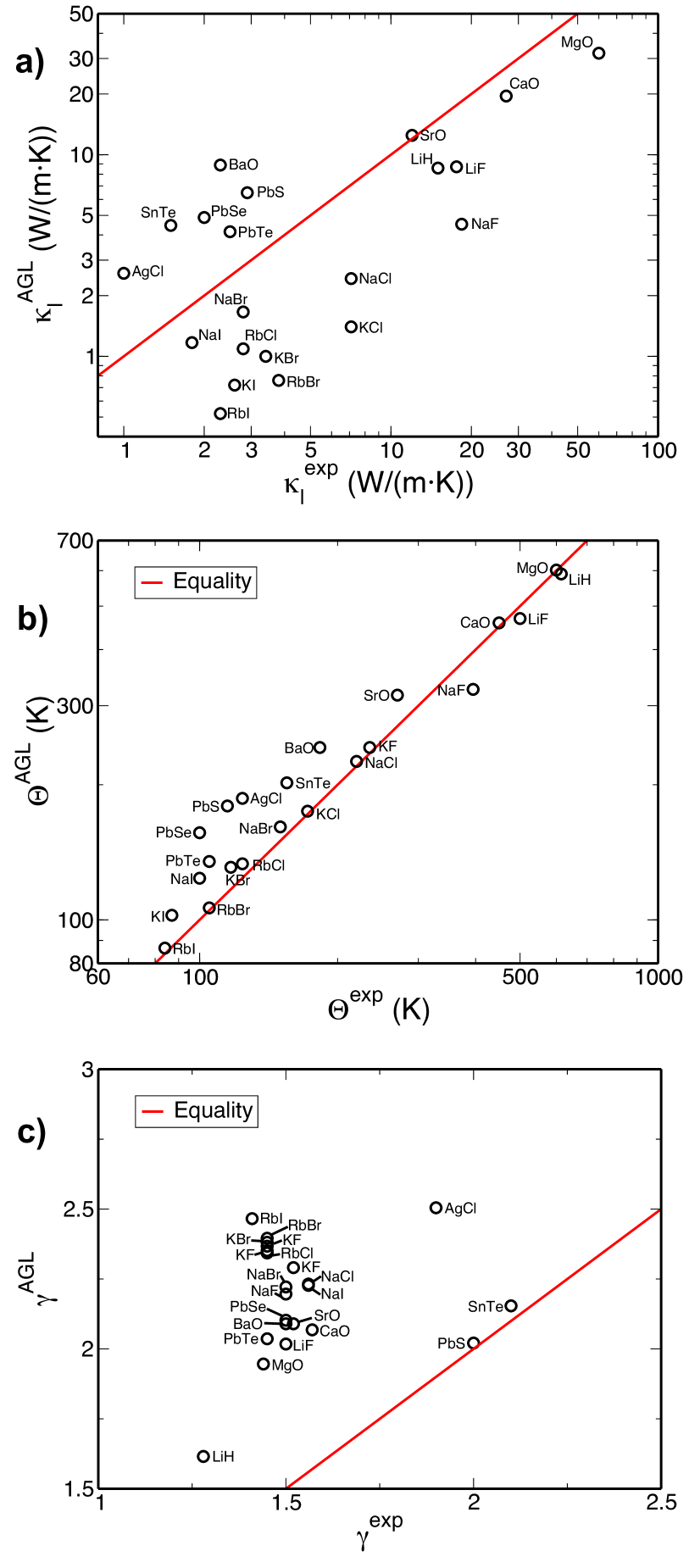
Figure 2: (a) Lattice thermal conductivity at 300K, (b) Debye temperature and (c) Grüneisen parameter of Rocksalt structure semiconductors. The Debye temperatures plotted in (b) are $\theta_{\mathrm{a}}$, except for SnTe where $\theta_{\mathrm{D}}$ is quoted in Ref. Snyder_jmatchem_2011, .

Table 2.1 of Ref. Morelli_Slack_2006, includes values of the thermal conductivity at 300K, calculated using the experimental values of $\theta_{\mathrm{a}}$ and $\gamma$. The Pearson correlation between these calculated thermal conductivities and their experimental values is $0.986$, and the corresponding Spearman correlation is $0.761$. Comparing these values with the correlations obtained using the AGL calculated quantities, we find that the latter are more significantly degraded than for the Diamond and Zincblende structures. This is despite the similar correlations obtained for $\theta_{\mathrm{a}}$ and $\gamma$ in these two cases. Nevertheless, the Pearson correlation between the calculated and experimental conductivities is high in both calculations, indicating that the AGL approach may be used as a screening tool for high conductivity compounds in cases where gaps exist in the experimental data for these materials.

III.3 Wurzite structure materials

Table 3: Lattice thermal conductivity at 300K, Debye temperature and Grüneisen parameter of Wurzite structure semiconductors. The experimental Debye temperature values listed are $\theta_{\mathrm{a}}$, except 190K for InSe Snyder_jmatchem_2011 and 660K for InN Ioffe_Inst_DB ; Krukowski_jphyschemsolids_1998 which are $\theta_{\mathrm{D}}$. Units: $\theta$ in (K), $\kappa$ in (W/(m$\cdot$K)).

Comp.	$\theta^{\mathrm{exp}}$	$\theta_{\mathrm{a}}^{\small AGL}$	$\theta_{\mathrm{D}}^{\small AGL}$	$\gamma^{\mathrm{exp}}$	$\gamma^{\small AGL}$	$\kappa^{\mathrm{exp}}$	$\kappa^{\small AGL}$
SiC	740 Morelli_Slack_2006	750	1191	0.75 Morelli_Slack_2006	1.86	490 Morelli_Slack_2006	52.63
AlN	620 Morelli_Slack_2006	485	770	0.7 Morelli_Slack_2006	1.85	350 Morelli_Slack_2006	32.58
GaN	390 Morelli_Slack_2006	291	462	0.7 Morelli_Slack_2006	2.07	210 Morelli_Slack_2006	14.55
ZnO	303 Morelli_Slack_2006	519	824	0.75 Morelli_Slack_2006	1.97	60 Morelli_Slack_2006	20.98
BeO	809 Morelli_Slack_2006	784	1244	1.38 Slack_JAP_1975 ; Cline_JAP_1967 ; Morelli_Slack_2006	1.76	370 Morelli_Slack_2006	44.6
				0.75 Morelli_Slack_2006
CdS	135 Morelli_Slack_2006	146	231	0.75 Morelli_Slack_2006	2.14	16 Morelli_Slack_2006	3.59
InSe	190 Snyder_jmatchem_2011	106	212	1.2 Snyder_jmatchem_2011	2.24	6.9 Snyder_jmatchem_2011	1.72
InN	660 Ioffe_Inst_DB ; Krukowski_jphyschemsolids_1998	202	321	0.97 Krukowski_jphyschemsolids_1998	2.17	45 Ioffe_Inst_DB ; Krukowski_jphyschemsolids_1998	8.04

Experimental results for Wurzite structure materials (spacegroup: $P6_{3}mc\ (\#186)$; Pearson symbol: $hP4$) appear in Table 2.3 of Ref. Morelli_Slack_2006, . Their comparison with our calculation results is shown in Table 3 and Figure 3. As was the case for the zincblende and wurzite structure materials, we have included the AGL results for both $\theta_{\mathrm{D}}$ and $\theta_{\mathrm{a}}$ in the table, while the AGL $\theta_{\mathrm{a}}$ was used for plotting Figure 3 and calculating the correlations. The experimental values listed in the table are all for $\theta_{\mathrm{a}}$ Morelli_Slack_2006 , with the exceptions of the values of 190K for InSe Snyder_jmatchem_2011 and 660K for InN Ioffe_Inst_DB ; Krukowski_jphyschemsolids_1998 , which are for $\theta_{\mathrm{D}}$. The AGL $\theta_{\mathrm{a}}$ values were used for plotting and correlation calculations, with the exception of that those for InSe and InN where $\theta_{\mathrm{D}}$ was used for plotting Figure 3b and for calculating the correlation between the Debye temperatures.

The Pearson correlation between the AGL thermal conductivity values and the experimental values is $0.943$. The corresponding Spearman correlation is $0.976$. The Spearman correlation between the experimental values of the thermal conductivity and the calculated values of $\theta_{\mathrm{a}}$ is $0.905$. The Pearson correlation between the experimental and calculated values of the Debye temperature is $0.8$, and the corresponding Spearman correlation is $0.833$. The correlations for the Grüneisen parameter are both poor, with Pearson and Spearman values of $-0.039$ and $0.160$, respectively.

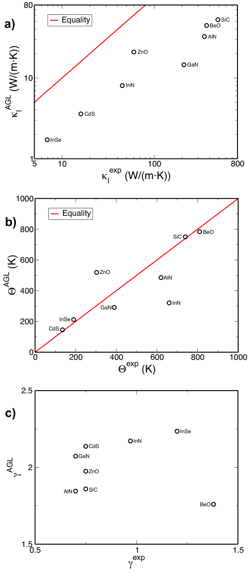
Figure 3: (a) Lattice thermal conductivity at 300K, (b) Debye temperature and (c) Grüneisen parameter of Wurzite structure semiconductors. The Debye temperatures plotted in (b) are $\theta_{\mathrm{a}}$, except for InSe and InN where $\theta_{\mathrm{D}}$ values are quoted in Refs. Snyder_jmatchem_2011, ; Ioffe_Inst_DB, ; Krukowski_jphyschemsolids_1998, .

Table 2.3 of Ref. Morelli_Slack_2006, includes values of the thermal conductivity at 300K, calculated using the experimental values of the Debye temperature and Grüneisen parameter. The Pearson correlation between these calculated thermal conductivity values and the experimental values is $0.996$, and the corresponding Spearman correlation is $1.0$. These values are again higher than the correlations obtained using the AGL calculated quantities, however, all of these correlations are very high so either of the calculation methods could serve as a reliable screening tool of the thermal conductivity. It should be noted that the high correlations calculated with the experimental $\theta_{\mathrm{a}}$ and $\gamma$ were obtained using $\gamma=0.75$ for BeO. Table 2.3 of Ref. Morelli_Slack_2006, also cites an alternative value of $\gamma=1.38$ for BeO (Table 3). Using this outlier value would severely degrade the results down to $0.7$, for the Pearson correlation, and $0.829$, for the Spearman correlation. These values are too low for a reliable screening tool. This demonstrates the ability of the AGL calculations to compensate for anomalies in the experimental data when they exist and still provide a reliable screening method for the thermal conductivity.

III.4 Rhombohedral materials

Experimental results for rhombohedral materials (spacegroups: $R\overline{3}mR\ (\#166)$, $R\overline{3}mH\ (\#166)$ and $R\overline{3}cH\ (\#167)$; Pearson symbols: $hR5$, $hR10$) are compared to the results of our calculations in Table 4 and Figure 4. The experimental Debye temperatures are for $\theta_{\mathrm{D}}$ in the case of Bi₂Te₃ and Sb₂Te₃, and for $\theta_{\mathrm{a}}$ in the case of Al₂O₃. The Pearson correlation between the experimental and calculated thermal conductivity values is $0.892$. The corresponding Spearman correlation is $0.600$. The Spearman correlation between the experimental values of the thermal conductivity and the values of $\theta_{\mathrm{a}}$ calculated with AGL is $0.943$.

Table 4: Lattice thermal conductivity at 300K, Debye temperature and Grüneisen parameter of rhombohedral semiconductors. The experimental Debye temperatures are $\theta_{\mathrm{D}}$ for Bi₂Te₃ and Sb₂Te₃, and $\theta_{\mathrm{a}}$ for Al₂O₃. Units: $\theta$ in (K), $\kappa$ in (W/(m$\cdot$K)).

Comp.	$\theta^{\mathrm{exp}}$	$\theta_{\mathrm{a}}^{\small AGL}$	$\theta_{\mathrm{D}}^{\small AGL}$	$\gamma^{\mathrm{exp}}$	$\gamma^{\small AGL}$	$\kappa^{\mathrm{exp}}$	$\kappa^{\small AGL}$
Bi2Te3	155 Snyder_jmatchem_2011	98	167	1.49 Snyder_jmatchem_2011	2.13	1.6 Snyder_jmatchem_2011	2.43
Sb2Te3	160 Snyder_jmatchem_2011	129	220	1.49 Snyder_jmatchem_2011	2.2	2.4 Snyder_jmatchem_2011	2.94
Al2O3	390 slack	376	810	1.32 slack	1.91	30 Slack_PR_1962	17.97
Cr2O3		262	565		2.26	16 Landolt-Bornstein ; Bruce_PRB_1977	8.59
Fe2O3		182	388		5.32	11.3 Landolt-Bornstein ; Horai_jgpr_1971	0.51
Bi2Se3		104	177		2.08	1.34 Landolt-Bornstein	2.88

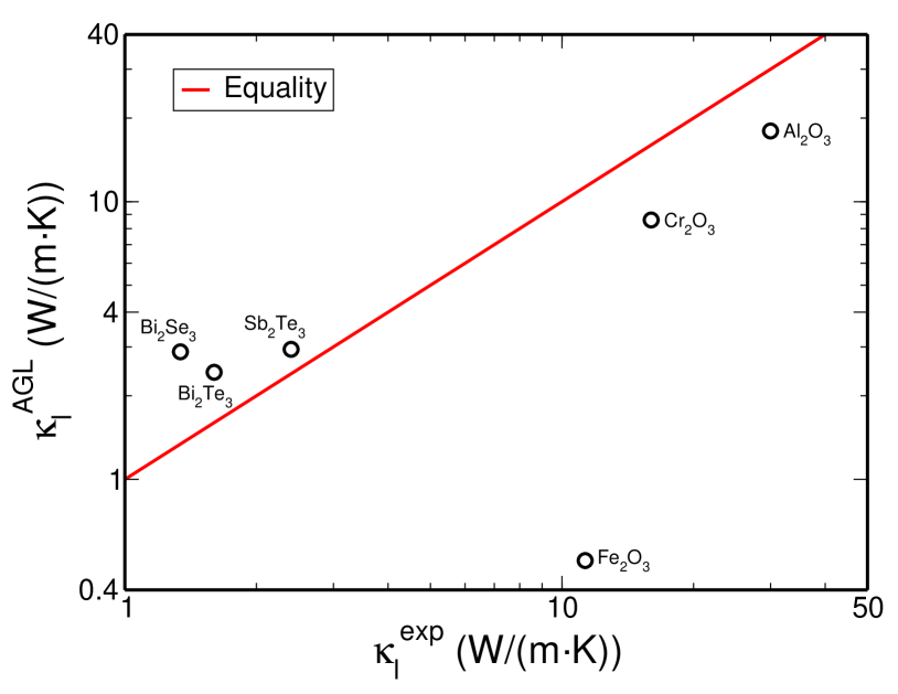
Figure 4: Lattice thermal conductivity of rhombohedral semiconductors at 300K.

The thermal conductivity of Fe₂O₃ is a clear outlier in this data set (see fig. 4). Its Grüneisen parameter, calculated with Equation (12), is $5.32$. It is abnormally high. Equation (11) gives a similar value of $5.36$, whereas Equation (16) gives a lower, but still very high, value of $4.06$. Ignoring Fe₂O₃ in the comparison increases the Pearson correlation of the calculated and experimental values of the thermal conductivity to $0.992$, while the Spearman correlation increases to $0.9$.

III.5 Body-centred tetragonal materials

Results for a set of body-centred tetragonal materials (spacegroup: $I\overline{4}2d\ (\#122)$; Pearson symbol: $tI16$) are shown in Table 5 and in Figure 5. For the materials ZnGeP₂ and AgGaS₂ there are three and two experimental values listed for $\kappa^{\mathrm{exp}}$. This is due to the materials having different thermal conductivities in different crystalline directionsBeasley_AO_1994 . The following results were obtained for the direction parallel to the optic axis, 36 W/(m$\cdot$K) and 1.4 W/(m$\cdot$K) for ZnGeP₂ and AgGaS₂, respectively. All of the experimental Debye temperatures listed in the table are the traditional Debye temperatures, $\theta_{\mathrm{D}}$.

Table 5: Lattice thermal conductivity at 300K, Debye temperature and Grüneisen parameter of body-centred tetragonal semiconductors. Units: $\theta$ in (K), $\kappa$ in (W/(m$\cdot$K)).

Comp.	$\theta_{\mathrm{D}}^{\mathrm{exp}}$	$\theta_{\mathrm{a}}^{\small AGL}$	$\theta_{\mathrm{D}}^{\small AGL}$	$\gamma^{\mathrm{exp}}$	$\gamma^{\small AGL}$	$\kappa^{\mathrm{exp}}$	$\kappa^{\small AGL}$
CuGaTe2	226 Snyder_jmatchem_2011	141	281	1.46 Snyder_jmatchem_2011	2.32	2.2 Snyder_jmatchem_2011	2.08
ZnGeP2	500 Landolt-Bornstein	176	351		2.13	35 Landolt-Bornstein ; Beasley_AO_1994	4.05
						36 Landolt-Bornstein ; Beasley_AO_1994
						18 Landolt-Bornstein ; Shay_1975 ; Masumoto_JPCS_1966
ZnSiAs2	347 Landolt-Bornstein ; Bohnhammel_PSSa_1981	155	309		2.15	14Landolt-Bornstein ; Shay_1975 ; Masumoto_JPCS_1966	3.37
CuInTe2	185 Landolt-Bornstein ; Rincon_PSSa_1995	119	237	0.93 Rincon_PSSa_1995	2.33	10Landolt-Bornstein ; Rincon_PSSa_1995	1.71
	195 Landolt-Bornstein ; Bohnhammel_PSSa_1982
AgGaS2	255 Landolt-Bornstein ; Abrahams_JCP_1975	135	269		2.20	1.4Landolt-Bornstein ; Beasley_AO_1994	2.52
						1.5Landolt-Bornstein ; Beasley_AO_1994
CdGeP2	340 Landolt-Bornstein ; Abrahams_JCP_1975	138	275		2.20	11 Landolt-Bornstein ; Shay_1975 ; Masumoto_JPCS_1966	2.84
CdGeAs2		140	280		2.20	42 Landolt-Bornstein ; Shay_1975	2.53
CuGaS2	356 Landolt-Bornstein ; Abrahams_JCP_1975	167	334		2.24	5.09 Landolt-Bornstein	3.3
CuGaSe2	262 Landolt-Bornstein ; Bohnhammel_PSSa_1982	154	307		2.27	12.9 Landolt-Bornstein ; Rincon_PSSa_1995	2.64
ZnGeAs2		147	294		2.16	11Landolt-Bornstein ; Shay_1975	2.93

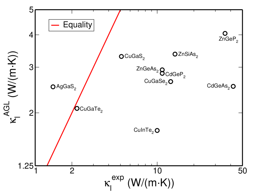
Figure 5: Lattice thermal conductivity of body-centred tetragonal semiconductors at 300K.

The Pearson correlation between the AGL thermal conductivity values and the experimental values is $0.383$. The corresponding Spearman correlation is $0.498$. The Spearman correlation between the experimental values of the thermal conductivity and the calculated values of $\theta_{\mathrm{a}}$ is $0.401$. The low correlations for this set of materials are due to their anisotropic structure, where the materials display different thermal conductivities along different lattice directions. This demonstrates the limits of the isotropic approximation made in the GIBBS method.

III.6 Miscellaneous materials

The results for materials with various other structures are shown in Table 6. The materials are CoSb₃ and IrSb₃ (spacegroup: $Im\overline{3}\ (\#204)$; Pearson symbol: $cI32$), ZnSb (spacegroup: $Pbca\ (\#61)$; Pearson symbol: $oP16$), Sb₂O₃ (spacegroup: $Pccn\ (\#56)$; Pearson symbol: $oP20$), InTe (spacegroup: $Pm\overline{3}m\ (\#221)$; Pearson symbol: $cP2$), Bi₂O₃ (spacegroup: $P121/c1\ (\#14)$; Pearson symbol: $mP20$), and SnO₂ (spacegroup: $P42/mnm\ (\#136)$; Pearson symbol: $tP6$). The experimental Debye temperatures listed in the table are the traditional Debye temperatures, $\theta_{\mathrm{D}}$, with the exception of ZnSb for which it is $\theta_{\mathrm{a}}$.

Table 6: Lattice thermal conductivity at 300K, Debye temperature and Grüneisen parameter of materials with various structures at 300K. The experimental Debye temperatures are $\theta_{\mathrm{D}}$, except ZnSb for which it is $\theta_{\mathrm{a}}$. Units: $\theta$ in (K), $\kappa$ in (W/(m$\cdot$K)).

Comp.	Pearson	$\theta^{\mathrm{exp}}$	$\theta_{\mathrm{a}}^{\small AGL}$	$\theta_{\mathrm{D}}^{\small AGL}$	$\gamma^{\mathrm{exp}}$	$\gamma^{\small AGL}$	$\kappa^{\mathrm{exp}}$	$\kappa^{\small AGL}$
CoSb3	$cI32$	307 Snyder_jmatchem_2011	150	378	0.95 Snyder_jmatchem_2011	2.63	10 Snyder_jmatchem_2011	2.02
IrSb3	$cI32$	308 Snyder_jmatchem_2011	96	241	1.42 Snyder_jmatchem_2011	2.34	16 Snyder_jmatchem_2011	2.25
ZnSb	$oP16$	92 Madsen_PRB_2014	85	214	0.76 Madsen_PRB_2014	2.24	3.5 Madsen_PRB_2014 ; Bottger_JEM_2010	1.09
Sb2O3	$oP20$		288	782		2.13	0.4 Landolt-Bornstein	6.07
InTe	$cP2$	186 Snyder_jmatchem_2011	152	191	1.0 Snyder_jmatchem_2011	2.28	1.7 Snyder_jmatchem_2011	3.12
Bi2O3	$mP20$		85	232		2.1	0.8 Landolt-Bornstein	2.09
SnO2	$tP6$		515	935		2.48	98Turkes_jpcss_1980	15.0
							55 Turkes_jpcss_1980

For these materials, the Pearson correlation between the calculated and experimental values of the thermal conductivity is $0.914$. The corresponding Spearman correlation is $0.071$. The Spearman correlation between the experimental values of the thermal conductivity and the calculated values of $\theta_{\mathrm{a}}$ is $0.143$.

The low correlation values, particularly for the Spearman correlation, for this set of materials demonstrates the importance of the information about the material structure as an input for the AGL method. This is partly due to the fact that the Grüneisen parameter tends not to vary significantly between materials with a particular structure, thus reducing its effect on the ordinal ranking of the thermal conductivity of materials with the same structure.

III.7 Half-Heusler materials

Carrete et al. curtarolo:art84 ; curtarolo:art85 studied the thermal conductivity of 107 half-Heusler (spacegroup: $F\overline{4}3m\ (\#216)$; Pearson symbol: $cF12$) compounds with ab initio and machine learning techniques. In this section we compare their results with our AGL calculations. We first consider a subset of these half-Heusler materials, taken from Table I of Ref. curtarolo:art84, , for which the thermal conductivity values were calculated using full anharmonic phonon parameterization solutions of the BTE. The thermal conductivities at 300K for this set of materials as calculated with Eq. (19) are shown in Table 7 and in Figure 6. The Pearson correlation between the AGL thermal conductivity values and the full anharmonic phonon calculations is $0.495$. The corresponding Spearman correlation is $0.810$. The Spearman correlation between the full anharmonic phonon calculation values of the thermal conductivity and the values of $\theta_{\mathrm{a}}$ as calculated with AGL is $0.730$. A major contributor to the low Pearson correlation is the outlier calculated value of the thermal conductivity of FeNbP and NiPbTi, 109.0 W/(m$\cdot$K) curtarolo:art84 . If these materials are removed from the dataset, the Pearson correlation increases to $0.629$.

Table 7: Thermal conductivities of half-Heusler semiconductors at 300K compared to full anharmonic phonon ab-initio parameterization from Ref. curtarolo:art84, . Units: $\theta$ in (K), $\kappa$ in (W/(m$\cdot$K)).

Comp.	$\theta_{\mathrm{a}}^{\small AGL}$	$\theta_{\mathrm{D}}^{\small AGL}$	$\gamma^{\small AGL}$	$\kappa^{\mathrm{anh}}$ [curtarolo:art84, ]	$\kappa^{\small AGL}$
AgKTe	105	152	2.26	0.508	1.0
BeNaP	302	436	2.05	4.08	5.3
BiBaK	95	137	1.94	2.19	1.59
BiKSr	99	143	1.96	1.96	1.45
BiLiSr	126	182	1.94	3.04	2.48
CoAsZr	306	442	2.14	24.0	17.51
CoBiHf	204	294	2.17	18.6	10.43
CoSbZr	231	333	3.00	25.0	4.69
CoScSe	230	331	2.09	15.0	6.64
CoSiTa	296	427	1.92	37.8	23.06
FeNbP	343	495	1.94	109.0	23.79
GeCaZn	197	284	2.05	2.75	4.53
GeNaY	189	273	2.04	8.06	4.28
LiBaSr	88	127	1.33	0.582	1.84
IrPTi	309	446	2.18	27.4	20.25
NiPbTi	205	296	2.20	109.0	7.35
NiSbSc	232	334	2.03	19.5	9.13
NiSnTi	249	359	2.06	17.9	10.7
NiSnZr	229	330	2.06	19.6	10.22
OsSbTa	227	328	2.14	29.6	16.62
PdAsY	230	332	2.17	5.48	9.43
PdSrTe	130	188	2.13	1.16	2.44
PtGaTa	242	349	2.19	32.9	16.78
PtGeTi	263	379	2.23	16.9	14.41
PtLaNb	140	202	2.69	16.5	2.2
RhHfSb	232	335	2.18	21.8	14.06
RhNbSi	345	497	2.09	15.3	26.15
RuAsV	334	482	2.19	23.5	21.37
SbCaK	141	203	1.92	2.70	2.47
SiCdSr	168	242	2.05	13.5	3.79
SnBaSr	114	165	1.71	2.01	3.19
TeAgLi	166	239	2.32	1.52	2.79

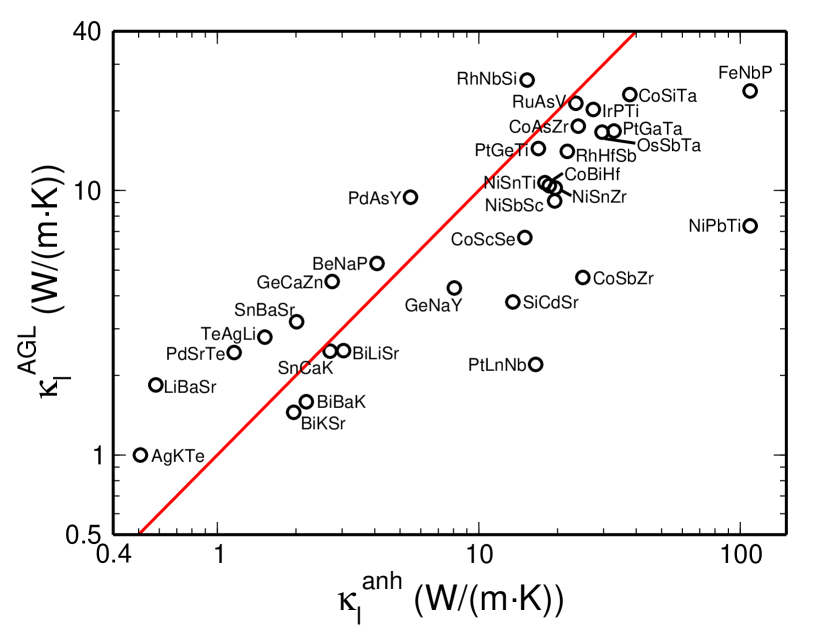
Figure 6: Thermal conductivities of half-Heusler semiconductors at 300K compared to full anharmonic phonon ab-initio parameterization from Ref. curtarolo:art84, .

The second subset of half-Heusler materials studied is taken from Table III of Ref. curtarolo:art84, , where the thermal conductivity was estimated using a machine learning algorithm. Comparison of these values with the thermal conductivity at 300K calculated with Eq. (19) is shown in Table 8 and Figure 7. The Pearson correlation between the AGL thermal conductivities and those produced by the machine learning algorithm is $0.578$. The corresponding Spearman correlation is $0.706$. The Spearman correlation between the machine learning thermal conductivities and the AGL values of $\theta_{\mathrm{a}}$ is $0.679$.

Table 8: Thermal conductivities of half-Heusler semiconductors at 300K compared to machine learning algorithm predictions from Ref. curtarolo:art84, . Units: $\theta$ in (K), $\kappa$ in (W/(m$\cdot$K)).

Comp.	$\theta_{\mathrm{a}}^{\small AGL}$	$\theta_{\mathrm{D}}^{\small AGL}$	$\gamma^{\small AGL}$	$\kappa^{\mathrm{ML}}$ [curtarolo:art84, ]	$\kappa^{\small AGL}$	Comp.	$\theta_{\mathrm{a}}^{\small AGL}$	$\theta_{\mathrm{D}}^{\small AGL}$	$\gamma^{\small AGL}$	$\kappa^{\mathrm{ML}}$ [curtarolo:art84, ]	$\kappa^{\small AGL}$
AuAlHf	217	313	2.12	16.7	12.14	NiBiSc	207	299	2.17	14.3	7.8
BLiSi	433	624	2.07	62.1	9.39	NiBiY	187	269	2.16	10.6	6.8
BiBaK	95	137	1.94	1.24	1.59	NiGaNb	289	417	2.11	22.9	14.79
CoAsHf	266	383	2.13	20.0	15.76	NiGeHf	238	343	2.02	19.6	13.05
CoAsTi	345	497	2.15	37.1	18.96	NiGeTi	330	476	2.10	25.3	17.56
CoAsZr	306	442	2.14	27.7	17.51	NiGeZr	295	426	2.07	21.1	16.78
CoBiHf	204	294	2.17	22.5	10.43	NiHfSn	230	332	2.08	19.5	12.97
CoBiTi	236	341	2.19	27.1	11.02	NiPbZr	195	281	2.19	15.2	7.5
CoBiZr	223	322	2.17	17.8	11.14	NiSnTi	249	359	2.06	16.8	10.7
CoGeNb	295	425	2.39	36.2	12.12	NiSnZr	229	330	2.06	17.5	10.22
CoGeTa	266	383	2.24	27.2	14.19	OsNbSb	254	367	2.12	24.8	19.38
CoGeV	334	482	2.01	29.1	20.26	OsSbTa	227	328	2.14	28.8	16.62
CoHfSb	190	274	1.69	21.9	12.18	PCdBa	198	285	2.24	6.05	3.45
CoNbSi	323	466	2.18	30.1	15.65	PdBiSc	194	280	2.23	9.95	7.22
CoNbSn	238	343	2.56	20.7	7.08	PdGeZr	267	385	2.18	18.2	14.04
CoSbTi	263	379	2.10	23.3	12.13	PdHfSn	218	314	2.21	15.1	11.35
CoSbZr	231	333	3.0	24.4	4.69	PdPbZr	203	293	2.29	10.3	8.72
CoSiTa	296	427	1.92	36.9	23.06	PtGaTa	242	349	2.19	32.3	16.78
CoSnTa	217	313	2.32	22.7	8.77	PtGeTi	263	379	2.23	26.7	14.41
CoSnV	266	383	2.49	19.8	8.47	PtGeZr	245	354	2.19	15.9	14.39
FeAsNb	339	489	2.13	47.6	23.09	PtLaSb	168	243	2.11	1.72	7.05
FeAsTa	295	425	2.13	32.9	21.08	RhAsTi	311	449	2.18	33.1	17.74
FeGeW	245	354	1.40	32.8	31.46	RhAsZr	284	409	2.17	27.1	16.73
FeNbSb	216	311	1.79	29.1	11.63	RhBiHf	182	263	2.25	12.8	8.01
FeSbTa	196	282	1.65	31.2	13.59	RhBiTi	228	329	2.25	13.0	11.1
FeSbV	305	440	1.50	24.1	39.0	RhBiZr	218	314	2.22	13.0	11.43
FeTeTi	266	384	2.24	26.2	11.02	RhLaTe	195	281	2.24	2.84	7.69
GeAlLi	270	390	2.06	16.5	6.36	RhNbSn	275	396	2.19	15.7	17.67
IrAsTi	277	399	2.22	30.1	16.92	RhSnTa	227	327	2.18	20.3	12.98
IrAsZr	255	368	2.19	17.4	16.04	RuAsNb	306	442	2.17	43.7	20.59
IrBiZr	206	297	2.24	12.8	11.67	RuAsTa	279	402	2.19	33.4	20.21
IrGeNb	279	402	2.17	33.0	20.88	RuNbSb	284	409	2.17	22.7	19.91
IrGeTa	256	369	2.15	37.2	20.43	RuSbTa	239	344	2.15	20.9	15.58
IrGeV	288	416	2.19	30.0	19.34	RuTeZr	241	348	2.26	21.3	11.76
IrHfSb	221	319	2.20	24.7	14.66	SbNaSr	139	200	1.90	3.49	2.83
IrNbSn	232	334	2.18	19.8	13.93	SiAlLi	363	523	2.02	20.9	9.26
IrSnTa	218	314	2.23	22.1	13.42	ZnLiSb	176	254	2.12	6.44	3.09
NiAsSc	300	432	2.11	17.5	13.32

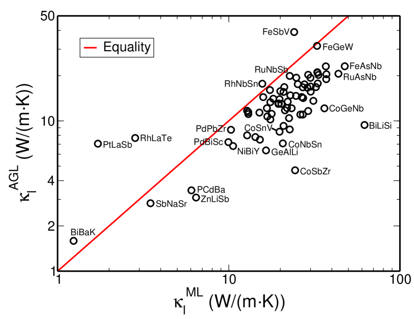
Figure 7: Thermal conductivities of half-Heusler semiconductors at 300K compared to machine learning algorithm predictions from Ref. curtarolo:art84, .

Table 9: Thermal conductivities of half-Heusler semiconductors at 300K compared to experimental values. Units: $\theta$ in (K), $\kappa$ in (W/(m$\cdot$K)).

Comp.	$\theta_{\mathrm{a}}^{\small AGL}$	$\theta_{\mathrm{D}}^{\small AGL}$	$\gamma^{\small AGL}$	$\kappa^{\mathrm{ML}}$ [curtarolo:art84, ]	$\kappa^{\small AGL}$	$\kappa^{\mathrm{exp}}$
CoHfSb	190	274	1.69	21.9	12.18	17Sekimoto2005
CoSbTi	263	379	2.10	23.3	12.13	12Kawaharada2004
						25Xia2000
CoSbZr	231	333	3.0	24.4	4.69	15Xia2000
FeSbV	305	440	1.50	24.1	39.0	13Young2000
NiHfSn	230	332	2.08	19.5	12.97	6.7Hohl1999
NiSnTi	249	359	2.06	16.8	10.7	9.3Hohl1999
NiSnZr	229	330	2.06	17.5	10.22	8.8Hohl1999
						17.2uher1999

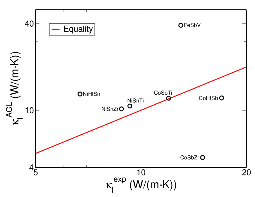
Figure 8: Thermal conductivities of half-Heusler semiconductors at 300K compared to experimental measurements.

Experimental results for the thermal conductivity of 7 of these half-Heusler materials were available in the literature, and these values are shown in Table 9 and Figure 8. The Pearson correlation between the AGL thermal conductivities and the experimental values is $0.064$, while the corresponding Spearman correlation is $-0.036$. The Spearman correlation between the experimental thermal conductivities and the AGL values of $\theta_{\mathrm{a}}$ is $0.0$. However, this is a small sample set, and these low correlation values appear to be primarily due to the outlier material CoSbZr, for which AGL predicts a relatively high value of $3.0$ for the Grüneisen parameter. Ignoring this material in the comparison increases the Pearson correlation between the thermal conductivities to $0.262$ and the Spearman correlation to $0.314$.

III.8 AGL predictions for zincblende materials

In order to demonstrate the potential utility of the AGL method for high-throughput screening of the thermal properties of materials we have calculated the Debye temperature, Grüneisen parameter and thermal conductivity for 45 zincblende structure (spacegroup: $F\overline{4}3m\ (\#216)$; Pearson symbol: $cF8$) materials which were not included in Table 1, and for which experimental values of the thermal conductivity do not seem to be available in the literature. The results for these materials are shown in Table 10 and in figure 9.

From these results, it is noticeable that BeO is predicted to have the highest thermal conductivity, with a value similar to that of SiC. This high thermal conductivity is in agreement with recent first principles calculations Li_JAP_BeO_2013 . Another set of materials predicted to have high thermal conductivity includes the nitrides PrN, ReN, NbN and MoN. Although BAs was previously predicted to have an extremely high thermal conductivity Lindsay_PRL_2013 , the AGL value is only slightly higher than that of Si or AlP, and less than that of BP, BN or SiC. The materials with the lowest thermal conductivity in this set are AgI and CuI. AgI, in particular, is predicted by AGL to have a thermal conductivity lower than that of any of the materials in Table 1.

Table 10: Lattice thermal conductivity at 300K, Debye temperature and Grüneisen parameter of Zincblende structure materials for which the experimental thermal conductivity is not available in the literature. Units: $\theta$ in (K), $\kappa$ in (W/(m$\cdot$K)).

Comp.	$\theta_{\mathrm{a}}^{\small AGL}$	$\theta_{\mathrm{D}}^{\small AGL}$	$\gamma^{\small AGL}$	$\kappa^{\small AGL}$	Comp.	$\theta_{\mathrm{a}}^{\small AGL}$	$\theta_{\mathrm{D}}^{\small AGL}$	$\gamma^{\small AGL}$	$\kappa^{\small AGL}$
AgI	123	155	2.45	1.51	MgSe	250	315	1.91	8.51
AgO	247	311	2.06	7.19	MgTe	187	236	1.94	5.57
AgSe	179	225	2.52	3.09	MoN	447	563	1.82	45.92
AuN	259	326	2.49	9.03	NbN	493	621	1.97	50.62
BAs	420	529	1.95	25.75	NiN	416	524	1.58	30.30
BeO	845	1065	1.74	62.77	PdN	387	487	2.37	18.2
BeS	506	637	1.76	27.54	PrN	309	389	1.27	58.21
BeSe	324	408	1.80	15.6	ReN	385	485	1.83	51.39
BeTe	237	299	1.85	9.77	RhN	450	567	2.27	29.91
CaSe	208	262	1.84	6.78	RuN	487	614	2.18	40.49
CdS	228	287	2.15	6.91	SbSn	143	180	1.70	5.52
CoO	427	538	2.41	14.46	ScSi	298	375	1.78	12.41
CuBr	190	239	2.44	2.94	ScSn	177	223	1.85	5.85
CuCl	234	295	2.40	3.76	SiP	357	450	2.97	4.90
CuF	272	343	2.34	4.66	TaN	379	477	1.97	41.64
CuI	161	203	2.48	2.45	TcB	371	468	1.59	35.46
GaBi	140	177	2.18	3.32	TcN	469	591	2.43	28.08
GdO	275	346	1.92	16.84	TiB	448	565	1.69	31.06
GeP	239	301	1.54	11.5	WN	344	433	2.44	19.76
GeSc	231	291	1.88	8.41	YN	373	470	1.80	28.51
HfN	348	439	1.89	36.14	ZnO	417	525	1.95	22.38
HgS	176	222	2.34	4.35	ZrN	450	567	1.92	41.65
IrN	371	467	2.19	31.79

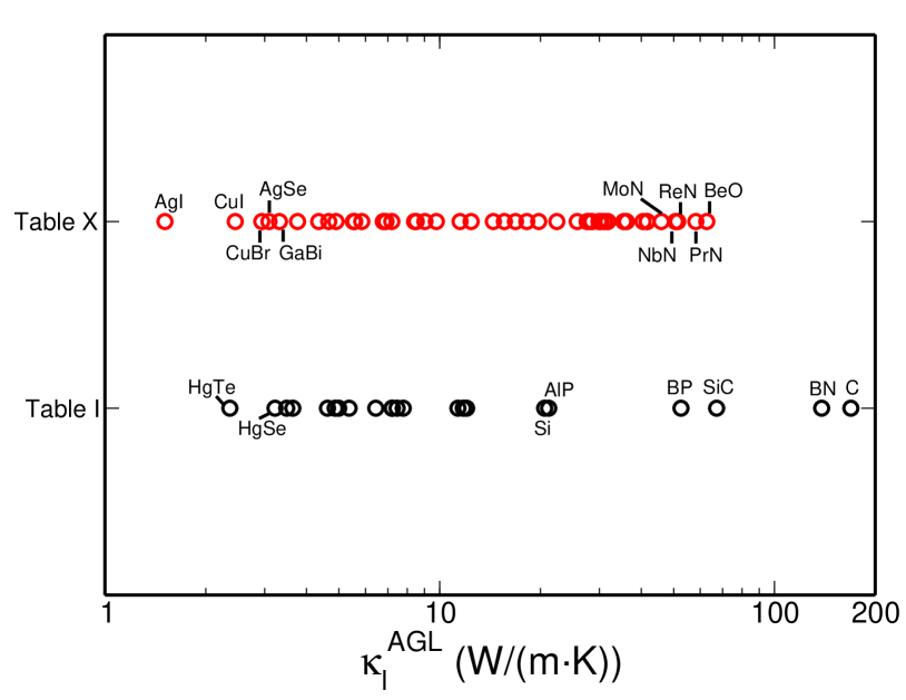
Figure 9: Predicted thermal conductivities of zincblende structure materials at 300K. The AGL values for the materials with experimental data listed in Table 1 are shown in black (see also figure 1). AGL predictions for materials with no experimental data are in red.

Table 11: Summary of correlations between experimental and AGL lattice thermal conductivity values. The total value is for the set containing all of the non-half Heusler materials.

Comp. set	Pearson	Spearman	Spearman
	$\kappa^{\mathrm{exp}}\!\!\leftrightarrow\!\kappa^{\small AGL}$	$\kappa^{\mathrm{exp}}\!\!\leftrightarrow\!\kappa^{\small AGL}$	$\kappa^{\mathrm{exp}}\!\!\leftrightarrow\!\theta_{\mathrm{a}}^{\small AGL}$
Zincblende	0.878	0.905	0.925
Rocksalt	0.910	0.445	0.645
Wurzite	0.943	0.976	0.905
Rhombohedral	0.892	0.600	0.943
Tetragonal	0.383	0.498	0.401
Misc.	0.914	0.071	0.143
Total	0.879	0.730	0.736

Table 12: Summary of correlations between ab initio and AGL lattice thermal conductivity values for the half Heusler materials.

Comp. set	Pearson	Spearman	Spearman
	$\kappa^{\mathrm{anh}}\!\!\leftrightarrow\!\kappa^{\small AGL}$	$\kappa^{\mathrm{anh}}\!\!\leftrightarrow\!\kappa^{\small AGL}$	$\kappa^{\mathrm{anh}}\!\!\leftrightarrow\!\theta_{\mathrm{a}}^{\small AGL}$
Full anharmonic	0.495	0.810	0.730
Machine learning	0.578	0.706	0.679

IV Conclusions

We implemented the “GIBBS” quasi-harmonic Debye model in the AGL  software package within the AFLOW and Materials Project high-throughput computational materials science frameworks. We used it to automatically calculate the thermal conductivity, Debye temperature and Grüneisen coefficient of materials with various structures and compared them with experimental results.

A major aim of high-throughput calculations is to identify useful markers (descriptors) for screening large datasets of structures for desirable properties curtarolo:art81 . In this study we examined whether the inexpensive-to-calculate Debye model thermal properties may be useful as such markers for high thermal conductivity materials, despite the well known deficiencies of this model in their quantitative evaluation. We therefore concentrated on correlations between the calculated quantities and the corresponding experimental data.

The correlations between the experimental values of the thermal conductivity and those calculated with AGL are summarized in Table 11. For the entire set of materials examined we find a high Pearson correlation of $0.879$ between $\kappa^{\mathrm{exp}}$ and $\kappa^{\small AGL}$. It is particularly high, above $0.9$, for materials with high symmetry (cubic or rhombohedral) structures, but significantly lower for anisotropic materials. We also compared these results with similar calculations of the thermal conductivity, using the experimental values of the Debye temperature and Grüneisen coefficient. The two methods gave similar Pearson correlations for the thermal conductivities, demonstrating that the AGL approach can rectify the lack of this experimental data in screening large data sets of materials.

The Spearman correlation between $\kappa^{\mathrm{exp}}$ and $\theta^{\small AGL}$ for the entire set of materials is almost as high as the Pearson correlation between the calculated and experimental conductivities. It is, however, less consistent for the high symmetry structures, with a relatively low value of $0.645$ for the Rocksalt structures. The Spearman correlation between $\kappa^{\mathrm{exp}}$ and $\kappa^{\small AGL}$ is found to be inferior to both previous measures as a descriptor of high conductivity materials. The correlations for the half-Heusler materials are summarized in Table 12.

Overall, despite the quantitative limitations of the method, the AGL approach can be useful for quickly screening large data sets of materials for favorable thermal properties.

V Acknowledgments

We thank Drs. Jesus Carrete, Natalio Mingo, Gus Hart, Anubhav Jain, Shyue Ping Ong, Kristin Persson, and Gerbrand Ceder for various technical discussions. We acknowledge support by the DOE (DE-AC02- 05CH11231), specifically the Basic Energy Sciences program under Grant # EDCBEE. The consortium AFLOWLIB.org acknowledges Duke University – Center for Materials Genomics — and the CRAY corporation for computational support.

References

- (1) M. Zebarjadi, K. Esfarjani, M. S. Dresselhaus, Z. F. Ren, and G. Chen, Perspectives on thermoelectrics: from fundamentals to device applications, Energy Environ. Sci. 5, 5147–5162 (2012).
- (2) J. Carrete, W. Li, N. Mingo, S. Wang, and S. Curtarolo, Finding unprecedentedly low-thermal-conductivity half-Heusler semiconductors via high-throughput materials modeling, Phys. Rev. X 4, 011019 (2014).
- (3) L.-T. Yeh and R. C. Chu, Thermal Management of Microloectronic Equipment: Heat Transfer Theory, Analysis Methods, and Design Practices (ASME Press, 2002).
- (4) C. D. Wright, L. Wang, P. Shah, M. M. Aziz, E. Varesi, R. Bez, M. Moroni, and F. Cazzaniga, The design of rewritable ultrahigh density scanning-probe phase-change memories, IEEE Trans. Nanotechnol. 10, 900–912 (2011).
- (5) K. Watari and S. L. Shinde, High thermal conductivity materials, MRS Bull. 26, 440–441 (2001).
- (6) G. A. Slack, R. A. Tanzilli, R. O. Pohl, and J. W. Vandersande, The intrinsic thermal conductivity of AlN, J. Phys. Chem. Solids 48, 641–647 (1987).
- (7) E. S. Toberer, A. Zevalkink, and G. J. Snyder, Phonon engineering through crystal chemistry, J. Mater. Chem. 21, 15843–15852 (2011).
- (8) D. A. Broido, M. Malorny, G. Birner, N. Mingo, and D. A. Stewart, Intrinsic lattice thermal conductivity of semiconductors from first principles, Appl. Phys. Lett. 91, 231922 (2007).
- (9) W. Li, N. Mingo, L. Lindsay, D. A. Broido, D. A. Stewart, and N. A. Katcho, Thermal conductivity of diamond nanowires from first principles, Phys. Rev. B 85, 195436 (2012).
- (10) G. Deinzer, G. Birner, and D. Strauch, Ab initio calculation of the linewidth of various phonon modes in germanium and silicon, Phys. Rev. B 67, 1443041–1443046 (2003).
- (11) A. Ward, D. A. Broido, D. A. Stewart, and G. Deinzer, Ab initio theory of the lattice thermal conductivity in diamond, Phys. Rev. B 80, 125203 (2009).
- (12) A. Ward and D. A. Broido, Intrinsic phonon relaxation times from first-principles studies of the thermal conductivities of Si and Ge, Phys. Rev. B 81, 085205 (2010).
- (13) Q. Zhang, F. Cao, K. Lukas, W. Liu, K. Esfarjani, C. Opeil, D. Broido, D. Parker, D. J. Singh, G. Chen, and Z. Ren, Study of the thermoelectric properties of lead selenide doped with Boron, gallium, indium, or thallium, J. Am. Chem. Soc. 134, 17731–17738 (2012).
- (14) W. Li, L. Lindsay, D. A. Broido, D. A. Stewart, and N. Mingo, Thermal conductivity of bulk and nanowire Mg2SixSn1-x alloys from first principles, Phys. Rev. B 86, 1743071–1743078 (2012).
- (15) L. Lindsay, D. A. Broido, and T. L. Reinecke, First-principles determination of ultrahigh thermal conductivity of boron arsenide: A competitor for diamond?, Phys. Rev. Lett. 111, 0259011–0259015 (2013).
- (16) L. Lindsay, D. A. Broido, and T. L. Reinecke, Ab initio thermal transport in compound semiconductors, Phys. Rev. B 87, 1652011–165220115 (2013).
- (17) J. M. Ziman, Electrons and Phonons: The Theory of Transport Phenomena in Solids (Oxford University Press, 2001).
- (18) J. Callaway, Model for Lattice Thermal Conductivity at Low Temperatures, Phys. Rev. 113, 1046–1051 (1959).
- (19) P. B. Allen, Zero-point and isotope shifts: Relation to thermal shifts, Phil. Mag. B 70, 527–534 (1994).
- (20) M. S. Green, Markoff random processes and the statistical mechanics of time-dependent phenomena. II. Irreversible processes in fluids, J. Chem. Phys. 22, 398–413 (1954).
- (21) R. Kubo, Statistical-mechanical theory of irreversible processes. I. General theory and simple applications to magnetic and conduction problems, J. Phys. Soc. Jpn. 12, 570–586 (1957).
- (22) S. Curtarolo, G. L. W. Hart, M. Buongiorno Nardelli, N. Mingo, S. Sanvito, and O. Levy, The high-throughput highway to computational materials design, Nat. Mater. 12, 191–201 (2013).
- (23) M. A. Blanco, E. Francisco, and V. Luaña, GIBBS: isothermal-isobaric thermodynamics of solids from energy curves using a quasi-harmonic Debye model, Comput. Phys. Commun. 158, 57–72 (2004).
- (24) S. Curtarolo, W. Setyawan, G. L. W. Hart, M. Jahnatek, R. V. Chepulskii, R. H. Taylor, S. Wang, J. Xue, K. Yang, O. Levy, M. Mehl, H. T. Stokes, D. O. Demchenko, and D. Morgan, AFLOW: an automatic framework for high-throughput materials discovery, Comp. Mat. Sci. 58, 218–226 (2012).
- (25) S. Curtarolo, W. Setyawan, S. Wang, J. Xue, K. Yang, R. H. Taylor, L. J. Nelson, G. L. W. Hart, S. Sanvito, M. Buongiorno Nardelli, N. Mingo, and O. Levy, AFLOWLIB.ORG: A distributed materials properties repository from high-throughput ab initio calculations, Comp. Mat. Sci. 58, 227–235 (2012).
- (26) R. H. Taylor, F. Rose, C. Toher, O. Levy, K. Yang, M. Buongiorno Nardelli, and S. Curtarolo, A RESTful API for exchanging Materials Data in the AFLOWLIB.org consortium, Comp. Mat. Sci. 93, 178–192 (2014).
- (27) A. Jain, G. Hautier, C. J. Moore, S. P. Ong, C. C. Fischer, T. Mueller, K. A. Persson, and G. Ceder, A high-throughput infrastructure for density functional theory calculations, Comp. Mat. Sci. 50, 2295–2310 (2011).
- (28) A. Jain, S. P. Ong, G. Hautier, W. Chen, W. D. Richards, S. Dacek, S. Cholia, D. Gunter, D. Skinner, G. Ceder, and K. A. Persson, Commentary: The Materials Project: A materials genome approach to accelerating materials innovation, APL Mater. 1, 011002 (2013).
- (29) S. P. Ong, W. D. Richards, A. Jain, G. Hautier, M. Kocher, S. Cholia, D. Gunter, V. L. Chevrier, K. A. Persson, and G. Ceder, Python Materials Genomics (pymatgen): A robust, open-source python library for materials analysis, Comp. Mat. Sci. 68, 314–319 (2013).
- (30) M. A. Blanco, A. M. Pendás, E. Francisco, J. M. Recio, and R. Franco, Thermodynamical properties of solids from microscopic theory: Applications to MgF2 and Al2O3, J. Mol. Struct., Theochem 368, 245–255 (1996).
- (31) J.-P. Poirier, Introduction to the Physics of the Earth’s Interior (Cambridge University Press, 2000), 2nd edn.
- (32) G. Kresse and J. Hafner, Ab initio molecular dynamics for liquid metals, Phys. Rev. B 47, 558–561 (1993).
- (33) P. E. Blöchl, Projector augmented-wave method, Phys. Rev. B 50, 17953–17979 (1994).
- (34) J. P. Perdew, K. Burke, and M. Ernzerhof, Generalized gradient approximation made simple, Phys. Rev. Lett. 77, 3865–3868 (1996).
- (35) H. J. Monkhorst and J. D. Pack, Special points for Brillouin-zone integrations, Phys. Rev. B 13, 5188–5192 (1976).
- (36) J. C. Slater, Introduction to Chemical Physics (McGraw-Hill, New York, 1939).
- (37) G. A. Slack, The thermal conductivity of nonmetallic crystals, in Solid State Physics, edited by H. Ehrenreich, F. Seitz, and D. Turnbull (Academic, New York, 1979), vol. 34, p. 1.
- (38) D. T. Morelli and G. A. Slack, High Lattice Thermal Conductivity Solids, in High Thermal Conductivity Materials, edited by S. L. Shindé and J. S. Goela (Springer, 2006).
- (39) D. Wee, B. Kozinsky, B. Pavan, and M. Fornari, Quasiharmonic Vibrational Properties of TiNiSn from Ab-Initio Phonons, J. Elec. Mat. 41, 977–983 (2012).
- (40) L. Bjerg, B. B. Iversen, and G. K. H. Madsen, Modeling the thermal conductivities of the zinc antimonides ZnSb and Zn4Sb3, Phys. Rev. B 89, 0243041–0243048 (2014).
- (41) Ioffe Physico - Technical Institute, http://www.ioffe.ru/SVA/NSM/Semicond/index.html.
- (42) Springer Materials: The Landolt-Börnstein Database, http://www.springermaterials.com/docs/index.html.
- (43) D. P. Spitzer, Lattice thermal conductivity of semiconductors: a chemical bond approach, J. Phys. Chem. Solids 31, 19–40 (1970).
- (44) C. R. Whitsett, D. A. Nelson, J. G. Broerman, and E. C. Paxhia, Lattice thermal conductivity of mercury selenide, Phys. Rev. B 7, 4625–4640 (1973).
- (45) M. A. ur Rehman and A. Maqsood, Measurement of Thermal Transport Properties with an Improved Transient Plane Source Technique, Int. J. Thermophys. 24, 867–883 (2003).
- (46) S. Krukowski, A. Witek, J. Adamczyk, J. Jun, M. Bockowski, I. Grzegory, B. Lucznik, G. Nowak, M. Wróblewski, A. Presz, S. Gierlotka, S. Stelmach, B. Palosz, S. Porowski, and P. Zinn, Thermal properties of indium nitride, J. Phys. Chem. Solids 59, 289–295 (1998).
- (47) G. A. Slack and S. F. Bartram, Thermal expansion of some diamond-like crystals, J. Appl. Phys. 46, 89–98 (1975).
- (48) C. F. Cline, H. L. Dunegan, and G. W. Henderson, Elastic Constants of Hexagonal BeO, ZnS, and CdSe, J. Appl. Phys. 38, 1944–1948 (1967).
- (49) G. A. Slack, Thermal conductivity of MgO, Al2O3, MgAl2O4, and Fe3O4 crystals from to K, Phys. Rev. 126, 427–441 (1962).
- (50) R. H. Bruce and D. S. Cannell, Specific heat of Cr2O3 near the Néel temperature, Phys. Rev. B 15, 4451–4459 (1977).
- (51) K. i. Horai, Thermal conductivity of rock-forming minerals, J. Geophys. Res. 76, 1278–1308 (1971).
- (52) J. D. Beasley, Thermal conductivities of some novel nonlinear optical materials, Applied Optics 33, 1000–1003 (1994).
- (53) J. L. Shay and J. H. Wernick, Ternary Chalcopyrite Semiconductors: Growth, Electronic Properties, and Applications (Pergamon, 1975), \doi10.1016/B978-0-08-017883-7.50002-0.
- (54) K. Masumoto, S. Isomura, and W. Goto, The preparation and properties of ZnSiAs2, ZnGeP2 and CdGeP2 semiconducting compounds, J. Phys. Chem. Solids 27, 1939–1947 (1966).
- (55) K. Bohmhammel, P. Deus, and H. A. Schneider, Specific heat, Debye temperature, and related properties of compound semiconductors AIIBIVC, Phys. Stat. Solidi A 65, 563–569 (1981).
- (56) C. Rincón, M. L. Valeri-Gil, and S. M. Wasim, Room-Temperature Thermal Conductivity and Grüneisen Parameter of the I–III–VI2 Chalcopyrite Compounds, Phys. Stat. Solidi A 147, 409–415 (1995).
- (57) K. Bohmhammel, P. Deus, G. Kühn, and W. Möller, Specific Heat, Debye Temperature, and Related Properties of Chalcopyrite Semiconducting Compounds CuGaSe2, CuGaTe2, CuInTe2, Phys. Stat. Solidi A 71, 505–510 (1982).
- (58) S. C. Abrahams and F. S. L. Hsu, Debye temperatures and cohesive properties, J. Chem. Phys. 63, 1162–1165 (1975).
- (59) P. H. M. Böttger, K. Valset, S. Deledda, and T. G. Finstad, Influence of Ball-Milling, Nanostructuring, and Ag Inclusions on Thermoelectric Properties of ZnSb, J. Elec. Mat. 39, 1583 (2010).
- (60) P. Türkes, C. Pluntke, and R. Helbig, Thermal conductivity of SnO2 single crystals, J. Phys. C: Solid State Phys. 13, 4941–4951 (1980).
- (61) J. Carrete, N. Mingo, S. Wang, and S. Curtarolo, Nanograined half-Heusler semiconductors as advanced thermoelectrics: an ab-initio high-throughput study, submitted (2014).
- (62) T. Sekimoto, K. Kurosaki, H. Muta, and S. Yamanaka, Thermoelectric poperties of (Ti,Zr,Hf)CoSb type half-Heusler compounds, Mater. Trans. 46, 1481–1484 (2005).
- (63) Y. Kawaharada, K. Kurosaki, H. Muta, M. Uno, and S. Yamanaka, High temperature thermoelectric properties of CoTiSb half-Heusler compounds, J. Alloys Compound. 384, 308–311 (2004).
- (64) Y. Xia, S. Bhattacharya, V. Ponnambalam, A. L. Pope, S. J. Poon, and T. M. Tritt, Thermoelectric properties of semimetallic (Zr, Hf)CoSb half-Heusler phases, J. Appl. Phys. 88, 1952–1955 (2000).
- (65) D. P. Young, P. Khalifah, R. J. Cava, and A. P. Ramirez, Thermoelectric properties of pure and doped FeMSb (M=V,Nb), J. Appl. Phys. 87, 317–321 (2000).
- (66) H. Hohl, A. P. Ramirez, C. Goldmann, G. Ernst, B. Wölfing, and E. Bucher, Efficient dopants for ZrNiSn-based thermoelectric materials, J. Phys.: Conden. Matt. 11, 1697–1709 (1999).
- (67) C. Uher, J. Yang, S. Hu, D. T. Morelli, and G. P. Meisner, Transport properties of pure and doped MNiSn (M=Zr, Hf), Phys. Rev. B 59, 8615–8621 (1999).
- (68) W. Li and N. Mingo, Thermal conductivity of bulk and nanowire InAs, AlN, and BeO polymorphs from first principles, J. Appl. Phys. 114, 183505 (2013).