Spectral and Energy Spectral Efficiency Optimization of Joint Transmit and Receive Beamforming Based Multi-Relay MIMO-OFDMA Cellular Networks

Abstract

We first conceive a novel transmission protocol for a multi-relay multiple-input–multiple-output orthogonal frequency-division multiple-access (MIMO-OFDMA) cellular network based on joint transmit and receive beamforming. We then address the associated network-wide spectral efficiency (SE) and energy spectral efficiency (ESE) optimization problems. More specifically, the network’s MIMO channels are mathematically decomposed into several effective multiple-input–single-output (MISO) channels, which are essentially spatially multiplexed for transmission. Hence, these effective MISO channels are referred to as spatial multiplexing components (SMCs). For the sake of improving the SE/ESE performance attained, the SMCs are grouped using a pair of proposed grouping algorithms. The first is optimal in the sense that it exhaustively evaluates all the possible combinations of SMCs satisfying both the semi-orthogonality criterion and other relevant system constraints, whereas the second is a lower-complexity alternative. Corresponding to each of the two grouping algorithms, the pair of SE and ESE maximization problems are formulated, thus the optimal SMC groups and optimal power control variables can be obtained for each subcarrier block. These optimization problems are proven to be concave, and the dual decomposition approach is employed for obtaining their solutions. Relying on these optimization solutions, the impact of various system parameters on both the attainable SE and ESE is characterized. In particular, we demonstrate that under certain conditions the lower-complexity SMC grouping algorithm achieves $90\%$ of the SE/ESE attained by the exhaustive-search based optimal grouping algorithm, while imposing as little as $3.5\%$ of the latter scheme’s computational complexity.

I Introduction

Recent wireless mobile broadband standards optionally employ relay nodes (RNs) and multiple-input–multiple-output orthogonal frequency-division multiple-access (MIMO-OFDMA) systems [1, 2] for supporting the ever-growing wireless capacity demands. These systems benefit from a capacity gain increasing roughly linearly both with the number of available OFDMA subcarriers (each having the same bandwidth) as well as with the minimum of the number of transmit antennas (TAs) and receive antennas (RAs). However, this capacity-oriented approach conflicts with the increasing need to reduce the system’s carbon footprint [3] as increasing the number of radio frequency (RF) chains and subcarriers will incur additional energy costs. In light of these discussions, the goal of this paper is to formally optimize the spectral efficiency (SE) or energy spectral efficiency (ESE) of the downlink (DL) in a multi-relay MIMO-OFDMA cellular system by intelligently allocating the available power and frequency resources and employing joint transmit and receive beamforming (BF).

It is widely acknowledged that under the idealized simplifying condition of having perfect channel state information (CSI) at the transmitter, the DL or broadcast channel (BC) capacity [4, 5] may be approached with the aid of dirty paper coding (DPC) [6]. However, the practical implementation of DPC is hampered by its excessive algorithmic complexity upon increasing the number of users. On the other hand, BF is an attractive suboptimal strategy for allowing multiple users to share the BC while resulting in reduced multi-user interference (MUI). A low-complexity transmit-BF technique is the zero-forcing based BF (ZFBF), which can asymptotically achieve the BC capacity as the number of users tends to infinity [7]. Furthermore, ZFBF may be readily applied to a system with multiple-antenna receivers through the use of the singular value decomposition (SVD). As a result, the associated MIMO channels may be mathematically decomposed into several effective multiple-input–single-output (MISO) channels, which are termed spatial multiplexing components (SMCs) in this work. Furthermore, in [8], these SMCs are specifically grouped so that the optimal grouping as well as the optimal allocation of the power may be found on each subcarrier block using convex optimization. In contrast to the channel-diagonalization methods of [9, 10, 11], the ZFBF approach does not enforce any specific relationship between the total numbers of TAs and RAs. Therefore, ZFBF is more suitable for practical systems, since the number of TAs at the BS is typically much lower than the total number of RAs of all the active user equipments (UEs). Compared to the random beamforming methods, such as that of [12], ZFBF is capable of completely avoiding the interference, allowing us to formulate our SE/ESE maximization (SEM/ESEM) problems as convex optimization problems. Due to its desirable performance versus complexity trade-off, in this paper we employ ZFBF in the context of multi-relay aided MIMO-OFDMA systems, where the direct link between the base station (BS) and the UE may be exploited in conjunction with the relaying link for further improving the system’s performance.

We formally define the ESE as a counterpart of the area spectral efficiency (ASE) [13], where the latter has the units of $\left[\mbox{bits/sec/Hz/m}^{2}\right]$, while the former is measured in $\left[\mbox{bits/sec/Hz/Joule}\right]$. The ESE metric has been justified, for example, in [14, 15, 16, 17]. However, these contributions did not consider resource allocation in the context of a MIMO system, and only [17] incorporated relaying. On the other hand, although there are numerous contributions on optimal resource allocation in MIMO systems, they typically only focused on either the SEM (equivalently, the sum-rate maximization) or the power minimization [8, 18, 19, 20, 21]. For example, the authors of [8] applied BF to a DL cellular system and aimed for minimizing the resultant total transmission power, while simultaneously satisfying the per-user rate requirements. The authors of [19] instead choose to minimize the per-antenna transmission powers, while satisfying both the maximum per-antenna power constraints as well as the per-user signal-to-noise-plus-interference (SINR) requirements. Although there exists some literature studying the ESE of relay-aided MIMO systems [22, 23], these contributions typically focus their attention on a simple three-node network consisting of the source, the destination and a single RN.

To summarize, there is a paucity of literature on the convex optimization approach to the ESEM problem associated with both resource allocation and joint transmit/receive beamforming in the context of multi-user multi-relay MIMO-OFDMA systems. Additionally, the Charnes-Cooper transformation [24] is employed in this paper for solving the associated ESEM problem, in contrast to the scalarization approach [25] that requires the weighting of multiple objectives. On the other hand, the Dinkelbach’s method [26, 14, 27, 17] is avoided as it would require solving a series of parametric convex problems, rather than the resultant single convex problem of the Charnes-Cooper transformation. Although the latter approach does impose an additional linear constraint on the problem, in our experience, this only marginally increases the complexity of the solution algorithm. The authors of [28] employed the Charnes-Cooper variable transformation for the ESEM of a simple point-to-point link. However, as far as we are aware, the Charnes-Cooper transformation has rarely been used in other contexts for solving the ESEM problem.

Let us now summarize the above discussions and provide a concise list of the novel contributions of this paper:

• We consider a generalized multi-user multi-relay assisted MIMO-OFDMA cellular system model for the SEM/ESEM problems. To provide some justification, this system model accounts for both the direct links between the BS and the UEs, as well as the relaying links employing the decode-and-forward (DF) relaying protocol [29]. This system model is unlike that of [7, 8], which did not consider relaying, and it is also distinct from that of [22, 23], which only consider a single RN and a single UE. Additionally, we dispense with the constraint that the number of antennas at the BS needs to be greater or equal to the sum of the number of antennas at the UEs, which was assumed in [9, 10, 11]. Furthermore, this system model is built upon our previous work [17] as the network elements may now be equipped with an arbitrary number of antennas for improving the system’s SE or ESE performance.

• A sophisticated novel transmission protocol is proposed for improving the system’s SE/ESE performance. Since the multi-relay MIMO-OFDMA system model considered has not been studied in the context of the SEM/ESEM problems before, we develop a novel transmission protocol that exploits spatial multiplexing in both transmission phases while allowing both the direct and relaying links to be simultaneously active. Although this protocol does not benefit from a higher spatial degree of freedom than that of the conventional half-duplex relay based cooperative system, we glean more flexibility in choosing the best group of channels for each transmission phase, which leads to additional selection diversity. As a result, the achievable SE/ESE performance may be improved. Again, this protocol is distinct from that presented in [7, 8], since relaying is not considered in those works. Another benefit is that since spatial multiplexing is employed in conjunction with OFDMA, multiple data streams may be served using the same subcarrier block, while the transmit ZFBF is employed for avoiding the interference. Furthermore, the receive-BF matrices are designed with the aim of generating a number of SMCs that may be grouped for the purpose of increasing the attainable spatial multiplexing gain.

• Two SMC grouping algorithms are proposed. To elaborate, we present a pair of novel algorithms for grouping the SMCs transmissions. The possibility of relayed transmissions means that we have to partition each transmission period into two halves, one consisting of BS-to-UE and BS-to-RN links, and the other consisting of additional BS-to-UE as well as RN-to-UE links. As a result, the SMC-pairs of the two-hop relaying links are incomparable to the SMCs of the direct links in either the first or the second transmission phases. This is because, firstly the RNs are subject to their individual maximum transmission power constraints, and secondly they employ the DF protocol, which means that the information conveyed on the RN-to-UE link cannot be more than that conveyed on the BS-to-RN link. These challenging issues are resolved by the proposed grouping algorithms. The first grouping algorithm is optimal in the sense that it is based on exhaustive search over all the SMC groupings that satisfy the semi-orthogonality criterion, while the second algorithm constitutes a lower-complexity alternative. This complexity-reduction is achieved by a multi-stage SMC group construction process. In each stage, we firstly compute the orthogonal components with respect to the vectors contained in the tentative SMC group to be constructed using all the residual legitimate SMC vectors, and then insert the particular SMC vector that results in the orthogonal component having the highest norm into the SMC group to be constructed. In principle, this method is similar to that of [7, 8], but it has been appropriately adapted for the multi-relay cellular network considered under the above-mentioned particular constraints.

• The problems of choosing the SE- or ESE-optimal SMC groupings and their associated power control values are formulated and solved using convex optimization. In contrast to [8, 18, 19, 20, 21], the crucial objective of maximizing the ESE metric is employed, as motivated above. On the other hand, in contrast to [14, 15, 16], we consider a system that allows for simultaneous direct and relayed transmissions for the sake of increasing the attainable spatial multiplexing gain. Although there exist other methods of solving this ESEM problem [25, 14, 27, 17], we employ the Charnes-Cooper transformation [24] for obtaining the maximum ESE solution, as it exhibits a reduced complexity from having to solve only a single convex optimization problem.

The rest of this paper is organized as follows. Section II describes the multi-relay MIMO-OFDMA cellular network considered, while Section III characterizes our novel transmission protocol that allows for both direct and relaying links to be simultaneously and continuously activated. In Section IV, we elaborate on the aforementioned SMC grouping algorithms conceived for forming the sets of possible SMC transmission groups. The issue of finding the optimal SMC transmission groups and the optimal power control variables is then formulated as an optimization problem in Section V, which is then solved by using a number of variable transformations and relaxations. The performance of both our SMC grouping algorithms and of the SEM/ESEM solvers are characterized in Section VI. Finally, we present our conclusions and future research ideas in Section VII.

II System model

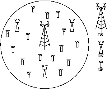
Figure 1: An example of a multi-relay MIMO-OFDMA cellular network, consisting of a single BS at the cell-center, 3 RNs and 15 UEs.

We focus our attention on the DL of a multi-relay MIMO-OFDMA cellular network, as shown in Fig. 1. The BS, $M$ DF-assisted RNs and $K$ UEs are each equipped with $N_{B}$, $N_{R}$ and $N_{U}$ antennas, respectively. The cellular system has access to $N$ subcarrier blocks, each encompassing $W$ Hertz of wireless bandwidth. The subcarrier blocks considered here are similar to the resource blocks in the LTE-nomenclature [30]. The BS is located at the cell-center, while the RNs are each located at a fixed distance from the BS and are evenly spaced around it. The ratio of the distance between the BS and RNs to the cell radius is denoted by $D_{r}$. On the other hand, the UEs are uniformly distributed in the cell. The BS coordinates and synchronizes its own transmissions with that of the RNs, which employ the DF protocol and thus avoids the problem of noise amplification. As it will be shown in Section V-C1, this strategy results in a simple algorithm for finding the optimal power control variables.

For the subcarrier block $n\in\left\{1,\cdots,N\right\}$, let us define the complex-valued wireless channel matrices between the BS and UE $k\in\left\{1,\cdots,K\right\}$, between the BS and RN $m\in\left\{1,\cdots,M\right\}$, and between RN $m$ and UE $k$ as $\mathbf{H}_{n,k}^{BU}\in\mathbb{C}^{N_{U}\times N_{B}}$, $\mathbf{H}_{n,m}^{BR}\in\mathbb{C}^{N_{R}\times N_{B}}$ and $\mathbf{H}_{n,m,k}^{RU}\in\mathbb{C}^{N_{U}\times N_{R}}$, respectively. These complex-valued channel matrices account for both the frequency-flat Rayleigh fading and the path-loss between the corresponding transceivers. The coherence bandwidth of each wireless link is assumed to be sufficiently high, so that each individual subcarrier block experiences frequency flat fading, although the level of fading may vary from one subcarrier block to another in each transmission period. Additionally, the transceivers are stationary or moving slowly enough so that the level of fading may be assumed to be fixed for the duration of a scheduled transmission period. Furthermore, the RAs are spaced sufficiently far apart, so that each TA/RA pair experiences independent and identically distributed (i.i.d.) fading. Since these channels are slowly varying, the system is capable of exploiting the benefits of channel reciprocity associated with time-division duplexing (TDD), so that the CSI becomes available at each BS- and RN-transmitter and at each possible RN- and UE-receiver. To elaborate, $\mathbf{H}_{n,k}^{BU}$ and $\mathbf{H}_{n,m}^{BR}$ are known at the BS, $\mathbf{H}_{n,m}^{BR}$ and $\mathbf{H}_{n,m,k}^{RU}$ are known at the RN $m$, while $\mathbf{H}_{n,k}^{BU}$ and $\mathbf{H}_{n,m,k}^{RU}$ are also known at UE $k$. Additionally, through the use of dedicated low-rate error-free feedback channels, $\mathbf{H}_{n,m,k}^{RU}$ is also assumed to be known at the BS so that the BS may perform network-wide scheduling. These channel matrices are assumed to have full row rank, which may be achieved with a high probability for typical DL wireless channel matrices.

Furthermore, each receiver suffers from additive white Gaussian noise (AWGN) having a power spectral density of $N_{0}$. The maximum instantaneous transmission power available to the BS and to each RN due to regulatory and health-constraints is $P_{max}^{B}$ and $P_{max}^{R}$, respectively. Since OFDMA modulation constitutes a linear operation, we focus our attention on a single subcarrier block and as usual, we employ the commonly-used equivalent baseband signal model.

III Transmission protocol design

The system can simultaneously use two transmission modes to convey information to the UEs, namely the BS-to-UE mode, and the relaying-based BS-to-RN and RN-to-UE mode. Note that although in classic OFDMA each data stream is orthogonal in frequency, for the sake of further improving the system’s attainable SE or ESE performance, our system employs spatial multiplexing in conjunction with ZFBF so that multiple data streams may be served using the same subcarrier block, without suffering from interference. Additionally, since the relaying-based transmission can be split into two phases, the design philosophy of the BF matrices in each phase are described separately, although for simplicity we have assumed that the respective channel matrices remain unchanged in both phases. Firstly, the definition of the semi-orthogonality criterion is given as follows [7].

Definition 1.

A pair of MISO channels, represented by the complex-valued column vectors $\mathbf{v}_{1}$ and $\mathbf{v}_{2}$, are said to be semi-orthogonal to each other with parameter $\alpha\in\left[0,1\right]$, when

$$\frac{\left|\Re\left(\mathbf{v}_{1}^{\mathrm{H}}\mathbf{v}_{2}\right)\right|}{\|\mathbf{v}_{1}\|\|\mathbf{v}_{2}\|}\leq\alpha.$$ (1)

To be more specific, a measure of the grade of orthogonality between $\mathbf{v}_{1}$ and $\mathbf{v}_{2}$ is given by the left-hand side of inequality (1), which ranges from $0$ for orthogonal vectors to $1$ for linearly dependent vectors.

The authors of [7] demonstrated that employing the ZFBF strategy for MISO channels that satisfy $\alpha\to 0$, while the number of users obeys $K\to\infty$, asymptotically achieves the DPC capacity, and it is therefore optimal for the BC channel. Similar principles are followed when maximizing the SE or ESE of the system considered in this paper.

III-A BF design for the first transmission phase

In the first transmission phase, only the BS is transmitting, while both the RNs and the UEs act as receivers. This is similar to the classic DL multi-user MIMO model. As described above, our aim is 1) to design a ZFBF matrix for the BS to avoid interference between data streams, and 2) to design receive BF matrices for the UEs and RNs so that the resultant effective DL channel matrices contain as many semi-orthogonal rows as possible that satisfy (1) for a given $\alpha$. Ideally, all receivers (UEs and RNs) should jointly compute their receive BF matrices to accomplish the second goal. However, this is generally impossible, since we cannot realistically assume that the channel matrices associated with each UE and RN are shared among them, due to the geographically-distributed nature of the UEs and RNs. As a compromise, we opt for guaranteeing that each individual effective DL channel matrix contains locally orthogonal rows by employing the SVD [7, 8]. Although these locally orthogonal rows may not remain orthogonal globally, they can be characterized using the semi-orthogonality metric of (1).

Bearing this in mind, the channel matrices of all DL transmissions originating from the BS are decomposed at the BS, UEs and RNs using the SVD [32] as $\mathbf{H}_{n,k}^{BU}=\mathbf{U}_{n,k}^{BU}\mathbf{S}_{n,k}^{BU}\left(\mathbf{V}_{n,k}^{BU}\right)^{\mathrm{H}}$ and $\mathbf{H}_{n,m}^{BR}=\mathbf{U}_{n,m}^{BR}\mathbf{S}_{n,m}^{BR}\left(\mathbf{V}_{n,m}^{BR}\right)^{\mathrm{H}}$, respectively. Thus, the receive-BF matrices for UE $k$ and RN $m$ are given by $\mathbf{R}_{n,k}^{BU,T_{1}}=\left(\mathbf{U}_{n,k}^{BU}\right)^{\mathrm{H}}\in\mathbb{C}^{N_{U}\times N_{U}}$ and $\mathbf{R}_{n,m}^{BR,T_{1}}=\left(\mathbf{U}_{n,m}^{BR}\right)^{\mathrm{H}}\in\mathbb{C}^{N_{R}\times N_{R}}$, and the effective DL channel matrices are then given by $\underline{\mathbf{H}}_{n,k}^{BU,T_{1}}=\mathbf{R}_{n,k}^{BU,T_{1}}\mathbf{H}_{n,k}^{BU}=\mathbf{S}_{n,k}^{BU}\left(\mathbf{V}_{n,k}^{BU}\right)^{\mathrm{H}}\in\mathbb{C}^{N_{U}\times N_{B}}$ and $\underline{\mathbf{H}}_{n,m}^{BR,T_{1}}=\mathbf{R}_{n,m}^{BR,T_{1}}\mathbf{H}_{n,m}^{BR}=\mathbf{S}_{n,m}^{BR}\left(\mathbf{V}_{n,m}^{BR}\right)^{\mathrm{H}}\in\mathbb{C}^{N_{R}\times N_{B}}$, respectively. Since $\mathbf{V}_{n,k}^{BU}$ and $\mathbf{V}_{n,m}^{BR}$ are both unitary, while $\mathbf{S}_{n,k}^{BU}$ and $\mathbf{S}_{n,m}^{BR}$ are both real and diagonal, these effective DL channel matrices respectively consist of $\min\left(N_{B},N_{U}\right)$ and $\min\left(N_{B},N_{R}\right)$ orthogonal non-zero rows with norms equal to their corresponding singular values. We refer to these non-zero orthogonal rows as the SMCs of their associated MIMO channel matrix . The $K$ BS-to-UE MIMO channel matrices and $M$ BS-to-RN channel matrices generate a total of $\left[K\cdot\min\left(N_{B},N_{U}\right)+M\cdot\min\left(N_{B},N_{R}\right)\right]$ SMCs. Since these SMCs are generated from independent MIMO channel matrices associated with geographically distributed UEs and RNs, they are not all guaranteed to be orthogonal to each other. Furthermore, since each UE or RN has multiple antennas and $N_{B}$ might not be sufficiently large to simultaneously support all UEs and RNs, we have to determine which specific SMCs should be served. As a result, for each two-phase transmission period, we opt for selecting a SMC group accounting for both phases from the set of available SMC groups. This selection process is achieved by jointly using the SMC grouping algorithm and solving the optimization problem detailed below. For the sake of clarity, the concepts of the SMC, of the SMC group and of the set of SMC groups are illustrated in Fig. 2.

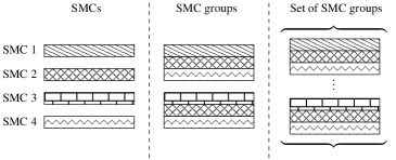
Figure 2: A conceptual illustration of the differences between SMCs, SMC groups and a set of SMC groups.

To elaborate a little further, a set of SMC groups, $\mathcal{G}_{n}$, which is associated with subcarrier block $n$, may be obtained using one of the grouping algorithms presented in Section IV. The BS selects a single group, $j\in\mathcal{G}_{n}$, containing (but not limited to $Q_{j}^{T_{1}}$ SMCs out of the $\left[K\cdot\min\left(N_{B},N_{U}\right)+M\cdot\min\left(N_{B},N_{R}\right)\right]$ available SMCs to be supported by using ZFBF. Thus, we have $Q_{j}^{T_{1}}\leq\min\left[N_{B},K\cdot\min\left(N_{B},N_{U}\right)+M\cdot\min\left(N_{B},N_{R}\right)\right]$ and a multiplexing gain of $Q_{j}^{T_{1}}$ is achieved. Let us denote the refined effective DL channel matrix with rows being the $Q_{j}^{T_{1}}$ selected SMCs as $\underline{\mathbf{H}}_{n,j}^{T_{1}}\in\mathbb{C}^{Q_{j}^{T_{1}}\times N_{B}}$. The ZFBF transmit matrix applied at the BS to subcarrier block $n$ is then given by the following right inverse $\mathbf{T}_{n,j}^{T_{1}}=\left(\underline{\mathbf{H}}_{n,j}^{T_{1}}\right)^{\mathrm{H}}\cdot\left[\underline{\mathbf{H}}_{n,j}^{T_{1}}\left(\underline{\mathbf{H}}_{n,j}^{T_{1}}\right)^{\mathrm{H}}\right]^{-1}\in\mathbb{C}^{N_{B}\times Q_{j}^{T_{1}}}$. Since $\underline{\mathbf{H}}_{n,j}^{T_{1}}\mathbf{T}_{n,j}^{T_{1}}=\mathbf{I}_{N_{B}}$, the potential interference between the $Q_{j}^{T_{1}}$ selected SMCs is completely avoided. Furthermore, the columns of $\mathbf{T}_{n,j}^{T_{1}}$ are normalized by multiplying the diagonal matrix $\mathbf{W}_{n,j}^{T_{1}}$ on the right-hand side of $\mathbf{T}_{n,j}^{T_{1}}$ to ensure that each SMC transmission is initially set to unit power.

Then, $\mathbf{T}_{n,j}^{T_{1}}\mathbf{W}_{n,j}^{T_{1}}$ is used as the DL transmit-BF matrix for the BS in the first phase. Thus, the effective channel-to-noise ratios (CNRs) in the first transmission phase can be written as $G_{n,j,e_{1}}^{BU,T_{1}}=\left|w_{n,j,e_{1}}^{BU,T_{1}}\right|^{2}/\Delta\gamma N_{0}W$ and $G_{n,j,e}^{BR,T_{1}}=\left|w_{n,j,e}^{BR,T_{1}}\right|^{2}/\Delta\gamma N_{0}W$, respectively, where $w_{n,j,e_{1}}^{BU,T_{1}}$ and $w_{n,j,e}^{BR,T_{1}}$ are the diagonal elements in $\mathbf{W}_{n,j}^{T_{1}}$. More specifically, these diagonal elements correspond to SMC group $j$ and subcarrier block $n$, and they are associated with either a direct BS-to-UE SMC or a BS-to-RN SMC. The additional subscripts $e_{1}\in\{0,\cdots,\min[N_{B},K\cdot\min(N_{B},N_{U})]\}$ and $e\in\{0,\cdots,\min[N_{B},M\cdot\min(N_{B},N_{R}),K\cdot\min(N_{R},N_{U})]\}$ are used for distinguishing the multiple selected SMCs of the direct links (i.e. those related to UEs), from the multiple selected SMC-pairs that may be associated with a particular RN $\mathcal{M}(e)$, respectively. Note that $\mathcal{M}\left(e\right)$ is a function of $e$, representing the RN index (similar to $m$ used before) associated with the SMC-pair $e$, as further detailed in Section IV.

At a given bit-error rate (BER) requirement, $\Delta\gamma$ is the signal-to-noise ratio (SNR) gap between the lower-bound SNR required for achieving the discrete-input–continuous-output memoryless channel (DCMC) capacity and the actual higher SNR required by the modulation/coding schemes of the practical physical layer transceivers employed. For example, making the simplifying assumption that idealized transceivers capable of achieving exactly the DCMC capacity are employed, then $\Delta\gamma=0\mbox{ dB}$. Although, strictly speaking, so far it is not possible to operate exactly at the DCMC channel capacity, there does exist several physical layer transceiver designs that operate very close to it [33]. Furthermore, the noise power received on each subcarrier block is given by $N_{0}W$.

III-B BF design in the second transmission phase

The second transmission phase may be characterized by the MIMO interference channel. A similar methodology is employed in the second transmission phase, except that now both the BS and the RNs are transmitters, while a number of UEs are receiving. In this phase, our aim is 1) to design ZFBF matrices for the BS and RNs to avoid interference between data streams, 2) and to design a receive-BF matrix for each UE so that the effective channel matrices associated with each of its transmitters contain rows which satisfy the semi-orthogonal condition (1) for a given $\alpha$. This means that more data streams may be served simultaneously, thus improving the attainable SE or ESE performance. Since there are multiple distributed transmitters/MIMO channel matrices associated with each UE, the SVD method described in Section III-A, which is performed in a centralized fashion, cannot be readily applied at the transmitter side. Instead, we aim for minimizing the resultant correlation between the generated SMCs, thus increasing the number of SMCs which satisfy (1) for a given $\alpha$. To accomplish this goal, we begin by introducing the shorthand of $\underline{\mathbf{H}}_{n,k}^{BU,T_{2}}=\mathbf{R}_{n,k}^{U,T_{2}}\mathbf{H}_{n,k}^{BU}\in\mathbb{C}^{N_{U}\times N_{B}}$ and $\underline{\mathbf{H}}_{n,m,k}^{RU,T_{2}}=\mathbf{R}_{n,k}^{U,T_{2}}\mathbf{H}_{n,m,k}^{RU}\in\mathbb{C}^{N_{U}\times N_{R}}$ as the effective channel matrices between the BS and UE $k$, and between RN $m$ and UE $k$, respectively, on subcarrier block $n$ in the second transmission phase, where $\mathbf{R}_{n,k}^{U,T_{2}}\in\mathbb{C}^{N_{U}\times N_{U}}$ is the yet-to-be-determined UE $k$’s receive-BF matrix. In light of the preceding discussions, one of our aims is to design $\mathbf{R}_{n,k}^{U,T_{2}}$ so that the off-diagonal values of the matrices given by $\mathbf{A}_{0}=\underline{\mathbf{H}}_{n,k}^{BU,T_{2}}\left(\underline{\mathbf{H}}_{n,k}^{BU,T_{2}}\right)^{\mathrm{H}}=\mathbf{R}_{n,k}^{U,T_{2}}\mathbf{H}_{n,k}^{BU}\left(\mathbf{H}_{n,k}^{BU}\right)^{\mathrm{H}}\left(\mathbf{R}_{n,k}^{U,T_{2}}\right)^{\mathrm{H}}$ and $\mathbf{A}_{m}=\underline{\mathbf{H}}_{n,m,k}^{RU,T_{2}}\left(\underline{\mathbf{H}}_{n,m,k}^{RU,T_{2}}\right)^{\mathrm{H}}=\mathbf{R}_{n,k}^{U,T_{2}}\mathbf{H}_{n,m,k}^{RU}\left(\mathbf{H}_{n,m,k}^{RU}\right)^{\mathrm{H}}\left(\mathbf{R}_{n,k}^{U,T_{2}}\right)^{\mathrm{H}}\mbox{, }\forall m$ are as small as possible. This design goal may be formalized as

$$\underset{\mathbf{R}_{n,k}^{U,T_{2}}}{\mbox{min. }} \left|\left|\mathbf{H}_{n,k}^{BU}\left(\mathbf{H}_{n,k}^{BU}\right)^{\mathrm{H}}-\left(\mathbf{R}_{n,k}^{U,T_{2}}\right)^{-1}\boldsymbol{\Lambda}_{0}\left(\mathbf{R}_{n,k}^{U,T_{2}}\right)^{\mathrm{-H}}\right|\right|_{\mathrm{F}}^{2}$$ (2)

$$+\sum_{m=1}^{M}\left|\left|\mathbf{H}_{n,m,k}^{RU}\left(\mathbf{H}_{n,m,k}^{RU}\right)^{\mathrm{H}}\right.\right.$$

$$\left.\left.-\left(\mathbf{R}_{n,k}^{U,T_{2}}\right)^{-1}\boldsymbol{\Lambda}_{m}\left(\mathbf{R}_{n,k}^{U,T_{2}}\right)^{\mathrm{-H}}\right|\right|_{\mathrm{F}}^{2},$$

where $\boldsymbol{\Lambda}_{0}$ and $\boldsymbol{\Lambda}_{m}$ are diagonal matrices containing the diagonal elements of $\mathbf{A}_{0}$ and $\mathbf{A}_{m}$, respectively. Therefore, $\left(\mathbf{R}_{n,k}^{U,T_{2}}\right)^{-1}$ is the jointly diagonalizing matrix [34], while $\mathbf{H}_{n,k}^{BU}\left(\mathbf{H}_{n,k}^{BU}\right)^{\mathrm{H}}$ and $\mathbf{H}_{n,m,k}^{RU}\left(\mathbf{H}_{n,m,k}^{RU}\right)^{\mathrm{H}}$, $\forall m$ are the matrices to be diagonalized. Thus, the algorithm presented in [34] for solving (2) may be invoked at UE $k$ for obtaining $\mathbf{R}_{n,k}^{U,T_{2}}$, which may be further fed back to the BS and RNs. Hence, the BS and RNs do not have to share ${\bf H}_{n,k}^{BU}$ or ${\bf H}_{n,k}^{RU}$ via the wireless channel and do not have to solve (2) again. As a result, we accomplish the goal of creating effective channel matrices that contain rows aiming to satisfy (1). Additionally, the columns of $\mathbf{R}_{n,k}^{U,T_{2}}$ have been normalized so that the power assigned for each SMC remains unaffected.

After obtaining the receive-BF matrix, the SMCs of the transmissions to UE $k$ on subcarrier block $n$ are given by the non-zero rows of the effective channel matrices $\underline{\mathbf{H}}_{n,k}^{BU,T_{2}}$ and $\underline{\mathbf{H}}_{n,m,k}^{RU,T_{2}}$, $\forall m$. Since the BS and the RNs act as distributed broadcasters in the second phase, they are only capable of employing separate ZFBF transmit matrices to ensure that none of them imposes interference on the SMCs it does not explicitly intend to serve. By employing one of the grouping algorithms described in Section IV, the BS schedules $Q_{j}^{T_{2}}\leq\min\left[\min\left(N_{B},N_{R}\right),\sum_{i=1}^{K}L_{i}^{B}+L_{i}^{R}\right]$ SMCs to serve simultaneously in the second phase, where $L_{i}^{B}$ and $L_{i}^{R}$ represent the number of SMCs of UE $i$ served by the BS and by RNs in this phase, respectively, where we have $L_{i}^{B}+L_{i}^{R}\leq N_{U}$, $L_{i}^{B}\leq\min(N_{B},N_{U})$, and $L_{i}^{R}\leq\min(N_{R},N_{U})$. Note that since UE $i$ may be simultaneously served both by the BS and by a RN (each of them serves a fraction of UE $i$’s SMCs), it is possible that the summation of the respective number of UEs served by the BS and by RNs may be higher than $K$. Let us denote the refined effective DL channel matrices, from the perspectives of the BS and RN $m$, consisting of the $Q_{j}^{T_{2}}$ selected SMCs as $\underline{\mathbf{H}}_{n,j}^{B,T_{2}}\in\mathbb{C}^{Q_{j}^{T_{2}}\times N_{B}}$ and $\underline{\mathbf{H}}_{n,j,m}^{R,T_{2}}\in\mathbb{C}^{Q_{j}^{T_{2}}\times N_{R}}$, respectively. Since these are known to each transmitter, they may employ ZFBF transmit matrices in the second phase, given by the right inverses $\mathbf{T}_{n,j}^{B,T_{2}}=\left(\underline{\mathbf{H}}_{n,j}^{B,T_{2}}\right)^{\mathrm{H}}\cdot\left[\underline{\mathbf{H}}_{n,j}^{B,T_{2}}\left(\underline{\mathbf{H}}_{n,j}^{B,T_{2}}\right)^{\mathrm{H}}\right]^{-1}\in\mathbb{C}^{N_{B}\times Q_{j}^{T_{2}}}$ for the BS, and $\mathbf{T}_{n,j,m}^{R,T_{2}}=\left(\underline{\mathbf{H}}_{n,j,m}^{R,T_{2}}\right)^{\mathrm{H}}\cdot\left[\underline{\mathbf{H}}_{n,j,m}^{R,T_{2}}\left(\underline{\mathbf{H}}_{n,j,m}^{R,T_{2}}\right)^{\mathrm{H}}\right]^{-1}\in\mathbb{C}^{N_{R}\times Q_{j}^{T_{2}}}$ for RN $m$. Similar to the first transmission phase, these ZFBF transmit matrices are normalized by $\mathbf{W}_{n,j}^{BU,T_{2}}$ and $\mathbf{W}_{n,j,m}^{RU,T_{2}}$, respectively, to ensure that each SMC transmission is initially set to unit power. Upon obtaining the selected SMCs, we denote the effective CNRs in the second transmission phase as $G_{n,j,e_{2}}^{BU,T_{2}}=\left|w_{n,j,e_{2}}^{BU,T_{2}}\right|^{2}/\Delta\gamma N_{0}W$ and $G_{n,j,e}^{RU,T_{2}}=\left|w_{n,j,e}^{RU,T_{2}}\right|^{2}/\Delta\gamma N_{0}W$, where $w_{n,j,e_{2}}^{BU,T_{2}}$ and $w_{n,j,e}^{RU,T_{2}}$ are the diagonal elements in $\mathbf{W}_{n,j}^{BU,T_{2}}$ and $\mathbf{W}_{n,j,\mathcal{M}(e)}^{RU,T_{2}}$, respectively, and the subscript $\mathcal{M}(e)$ has been defined in Section III-A. To elaborate, for a second-phase BS-to-UE link, $w_{n,j,e_{2}}^{BU,T_{2}}$ corresponds to SMC group $j$ and subcarrier block $n$, while the subscript $e_{2}\in\{0,\cdots,\min[N_{B},K\cdot\min(N_{B},N_{U})]\}$ is employed for further distinguishing the multiple selected SMCs associated with UEs from the BS. Similarly, $w_{n,j,e}^{RU,T_{2}}$, which also corresponds to SMC group $j$ and subcarrier block $n$, is associated with the second-phase RN-to-UE link between RN $\mathcal{M}\left(e\right)$ and the particular UE determined by the SMC-pair $e$.

Figure 3: A conceptual schematic of the transmit- and receive-BF matrices employed in the first and second transmission phases. In the first phase, the BS applies the ZFBF transmit matrix $\mathbf{T}_{n,j}^{T_{1}}$ in order to serve multiple data streams without imposing interference between them. In the second phase, the BS and RNs employ separate ZFBF matrices to distributively avoid interference between the data streams being served.

For more explicit clarity, a schematic of the transmit and receive beamforming matrices in the first and second transmission phases is presented in Fig. 3.

III-C Achievable spectral efficiency and energy spectral efficiency

$$C_{T}\left(\mathcal{P},\mathcal{S}\right)=\sum_{n=1}^{N}\sum_{j\in\mathcal{G}_{n}}s_{n,j}\left[\sum_{e_{1}\in\mathcal{E}_{n,j}}C_{n,j,e_{1}}^{BU,T_{1}}\left(\mathcal{P}\right)+\sum_{e_{2}\in\mathcal{E}_{n,j}}C_{n,j,e_{2}}^{BU,T_{2}}\left(\mathcal{P}\right)+\sum_{e\in\mathcal{E}_{n,j}}C_{n,j,e}^{BRU}\left(\mathcal{P}\right)\right].$$ (3)

$$P_{T}\left(\mathcal{P},\mathcal{S}\right) = \left(P_{C}^{B}+M\cdot P_{C}^{R}\right)+\frac{1}{2}\sum_{n=1}^{N}\sum_{j\in\mathcal{G}_{n}}s_{n,j}\Bigg{[}\xi^{B}\left(\sum_{e_{1}\in\mathcal{E}_{n,j}}P_{n,j,e_{1}}^{BU,T_{1}}+\sum_{e_{2}\in\mathcal{E}_{n,j}}P_{n,j,e_{2}}^{BU,T_{2}}\right)$$ (4)

$$+\sum_{e\in\mathcal{E}_{n,j}}\left(\xi^{B}P_{n,j,e}^{BR,T_{1}}+\xi^{R}P_{n,j,e}^{RU,T_{2}}\right)\Bigg{]}.$$

For the sake of convenience, let us first denote the transmit power allocation policy as $\mathcal{P}$, which is a set composed by all transmit power control variables invoked at the BS and/or RNs in both transmission phases. Since receive-BF is employed in conjunction with ZFBF, each SMC transmission may be viewed as a single-input–single-output (SISO) link. Therefore, on the direct links, the receiver’s SNR at UE $k$ corresponding to SMCs $e_{1}$ and $e_{2}$ may be expressed as $\Gamma_{n,j,e_{1}}^{BU,T_{1}}\left(\mathcal{P}\right)=G_{n,j,e_{1}}^{BU,T_{1}}P_{n,j,e_{1}}^{BU,T_{1}}$ and $\Gamma_{n,j,e_{2}}^{BU,T_{2}}\left(\mathcal{P}\right)=G_{n,j,e_{2}}^{BU,T_{2}}P_{n,j,e_{2}}^{BU,T_{2}}$ for the first and second transmission phases, respectively. The scalar variables $P_{n,j,e_{1}}^{BU,T_{1}}$ and $P_{n,j,e_{2}}^{BU,T_{2}}$, which are elements of $\mathcal{P}$, determine the transmit power values for SMCs $e_{1}$ and $e_{2}$ on the direct links. As a result, the achievable instantaneous SE of the direct links is given by $C_{n,j,e_{1}}^{BU,T_{1}}\left(\mathcal{P}\right)=\frac{1}{2}\log_{2}\left(1+\Gamma_{n,j,e_{1}}^{BU,T_{1}}\left(\mathcal{P}\right)\right)$ and $C_{n,j,e_{2}}^{BU,T_{2}}\left(\mathcal{P}\right)=\frac{1}{2}\log_{2}\left(1+\Gamma_{n,j,e_{2}}^{BU,T_{2}}\left(\mathcal{P}\right)\right)$, which are normalized both by time and by frequency to give units of $\left[\mbox{bits/sec/Hz}\right]$. The factor of $\frac{1}{2}$ accounts for the fact that the transmission period is split into two phases.

Similarly, for the SMC-pair $e$ of the DF relaying links, the SNR at RN $\mathcal{M}(e)$ in the first transmission phase is given by $\Gamma_{n,j,e}^{BR,T_{1}}\left(\mathcal{P}\right)=G_{n,j,e}^{BR,T_{1}}P_{n,j,e}^{BR,T_{1}}$ and the SNR at UE $k$ in the second transmission phase is formulated as $\Gamma_{n,j,e}^{RU,T_{2}}\left(\mathcal{P}\right)=G_{n,j,e}^{RU,T_{2}}P_{n,j,e}^{RU,T_{2}}$. Additionally, $P_{n,j,e}^{BR,T_{1}}$ and $P_{n,j,e}^{RU,T_{2}}$ are also elements of $\mathcal{P}$. Since the RNs employ the DF protocol, the achievable SE is limited by the weaker of the two RN-related links [29] and is given by $C_{n,j,e}^{BRU}\left(\mathcal{P}\right)=\min\left[\frac{1}{2}\log_{2}\left(1+\Gamma_{n,j,e}^{BR,T_{1}}\left(\mathcal{P}\right)\right),\frac{1}{2}\log_{2}\left(1+\Gamma_{n,j,e}^{RU,T_{2}}\left(\mathcal{P}\right)\right)\right]$.

Let us now introduce the SMC group selection variable $s_{n,j}\in\left\{0,1\right\}$, which indicates that SMC group $j$, as introduced in Sections III-A and III-B, is selected for subcarrier block $n$, when $s_{n,j}=1$, and $s_{n,j}=0$ otherwise. All SMC group selection variables are scalars and are collected into a set denoted by $\mathcal{S}$. Once again, we emphasize that $\mathcal{G}_{n}$ denotes the set of possible SMC groups for subcarrier block $n$. Thus, the total achieved SE is given by (3), where $\mathcal{E}_{n,j}$ is the set comprising the SMCs in the selected group $j$ on subcarrier block $n$.

In this work, we adopt the energy dissipation model presented in [36], where the total energy dissipation of the system is assumed to be dependent on several factors, including the number of TAs, the energy dissipation of the RF and baseband circuits, and the efficiencies of the power amplifier, feeder cables, cooling system, mains power supply, and converters. For the sake of simplicity, the total energy dissipation as presented in [36] has been partitioned into a fixed term, and a term that varies with the transmission powers. Thus, the energy dissipation of the system may be characterized by (4), where $P_{C}^{B}$ and $P_{C}^{R}$ represent the fixed energy dissipation of each BS and each RN, respectively, while $\xi^{B}>1$ and $\xi^{R}>1$ are the energy dissipation multipliers of the transmit powers for the BS and the RNs, respectively. The effect of multiple transmit antennas on the total energy dissipation has been included in the terms $P_{C}^{B}$, $P_{C}^{R}$, $\xi^{B}$ and $\xi^{R}$.

Finally, the ESE of the system is expressed as

$$\eta_{E}\left(\mathcal{P},\mathcal{S}\right)=\frac{C_{T}\left(\mathcal{P},\mathcal{S}\right)}{P_{T}\left(\mathcal{P},\mathcal{S}\right)}.$$ (5)

The objective of this paper is to maximize (5) by appropriately optimizing $\mathcal{P}$ and $\mathcal{S}$.

IV Semi-orthogonal grouping algorithms

As described in Section II, the BS has to choose $Q_{j}^{T_{1}}$ and $Q_{j}^{T_{2}}$ SMCs for the first and second transmission phases, respectively. These selected SMCs collectively form the SMC group $j$. Since the system supports both direct and relaying links, the grouping algorithms described in [7, 8], which were designed for MIMO systems dispensing with relays, may not be directly applied. Instead, we propose a pair of viable grouping algorithms, namely the exhaustive search-based grouping algorithm (ESGA), and the orthogonal component-based grouping algorithm (OCGA).

Note that because there are multiple distributed transmitters in the second transmission phase, each UE designs its receive-BF matrix by jointly considering all the MIMO channel matrices associated with it, as described in Section III-B. However, before applying this method, we have to determine which particular transmitters (out of the BS and RNs) should actively transmit in the second transmission phase based on the results of SMC selection. Note that it is possible that the SMC candidates obtained may lead to higher effective CNRs when a subset of the transmitters are inactive. On the one hand, an additional effect of only activating a subset of transmitters is the reduced number of SMC candidates, which might in turn result in a reduced number of qualified SMCs that satisfy the semi-orthogonality criterion considered. As a result, the achievable spatial multiplexing gain and SE might be degraded. On the other hand, this SE-reduction effect may be counteracted by the improved CNRs gleaned from the fact that it is easier to generate SMCs that can satisfy a stricter semi-orthogonality criterion, specified by a smaller value of $\alpha$, when the number of transmitters is lower. For example, in the scenarios where only one or two active transmitters are selected, the UEs can employ receive-BF matrices that create effective DL channel matrices containing completely orthogonal rows by using the SVD or the exact diagonalization method (see Footnote 11), respectively. In order to account for this dilemma, for the second transmission phase, the proposed grouping algorithms evaluate a full list of SMCs, which consists of the SMCs obtained from the $2^{M+1}-1$ possible combinations of active transmitters (the BS and $M$ RNs, while ignoring the case when there are no active transmitters). Compared to using a smaller list of SMCs, using a full list of SMCs ensures that achieving a lower-bound SE is always guaranteed, while a higher SE can only be obtained upon increasing the number of transmitters in the system.

IV-A SMC checking algorithm

inputs : candidate SMC $e_{c}$, current SMC group $\mathcal{E}_{n,j}$,
semi-orthogonality parameter $\alpha$

outputs : true or false

1 bool SMCCheck $\left(e_{c},\mathcal{E}_{n,j},\alpha\right)$ begin

2       $\mathcal{T}^{BS,T_{1}}\leftarrow\{\}$;

3       $\mathcal{T}^{BS,T_{2}}\leftarrow\{\}$;

4       $\mathcal{T}^{RN,T_{2}}_{m}\leftarrow\{\}\text{, }\forall m\in\{1,\cdots,M\}$;

5       $\mathcal{R}^{UE,T_{2}}_{k}\leftarrow\{\}\text{, }\forall k\in\{1,\cdots,K\}$;

6       foreach SMC $e_{1}\in\mathcal{E}_{n,j}$ do

7             $\mathcal{T}^{BS,T_{1}}\leftarrow\mathcal{T}^{BS,T_{1}}\cup\{e_{1}\}$;

8            

9       end foreach

10      foreach SMC $e_{2}\in\mathcal{E}_{n,j}$ do

11             $\mathcal{T}^{BS,T_{2}}\leftarrow\mathcal{T}^{BS,T_{2}}\cup\{e_{2}\}$;

12             $\mathcal{R}_{k}^{UE,T_{2}}\leftarrow\mathcal{R}_{k}^{UE,T_{2}}\cup\{e_{2}\}$;

13            

14       end foreach

15      foreach SMC $e\in\mathcal{E}_{n,j}$ do

16             $\mathcal{T}^{BS,T_{2}}\leftarrow\mathcal{T}^{BS,T_{2}}\cup\{e\}$;

17             $\mathcal{T}_{\mathcal{M}(e)}^{RN,T_{2}}\leftarrow\mathcal{T}_{\mathcal{M}(e)}^{RN,T_{2}}\cup\{e\}$;

18            

19       end foreach

20       if $e_{c}$ is BS transmission in $T_{1}$ then

21             $\mathcal{T}^{BS,T_{1}}\leftarrow\mathcal{T}^{BS,T_{1}}\cup\{e_{c}\}$;

22             if $\mathcal{T}^{BS,T_{1}}$ is not $\alpha$-semi-orthogonal or $|\mathcal{T}^{BS,T_{1}}|>N_{B}$ then return false ;

23            

24       else if $e_{c}$ is BS transmission in $T_{2}$ then

25             $\mathcal{T}^{BS,T_{2}}\leftarrow\mathcal{T}^{BS,T_{2}}\cup\{e_{c}\}$;

26             $\mathcal{T}^{RN,T_{2}}_{m}\leftarrow\mathcal{T}^{RN,T_{2}}_{m}\cup\{e^{\varnothing}_{m}\}\text{, }\forall m\in\{1,\cdots,M\}$;

27            

28       else if $e_{c}$ is RN $m$ transmission in $T_{2}$ then

29             $\mathcal{T}^{RN,T_{2}}_{m}\leftarrow\mathcal{T}^{RN,T_{2}}_{m}\cup\{e_{c}\}$;

30             $\mathcal{T}^{BS,T_{2}}\leftarrow\mathcal{T}^{BS,T_{2}}\cup\{e^{\varnothing}\}$;

31             $\mathcal{T}^{RN,T_{2}}_{m^{\prime}}\leftarrow\mathcal{T}^{RN,T_{2}}_{m^{\prime}}\cup\{e^{\varnothing}_{m^{\prime}}\}\text{, }\forall m^{\prime}\in\{1,\cdots,M\}\setminus m$;

32            

33       end if

34       if $\mathcal{T}^{BS,T_{2}}$ is not $\alpha$-semi-orthogonal or $|\mathcal{T}^{BS,T_{2}}|>N_{B}$ then  return false ;

35       if $\mathcal{T}^{RN,T_{2}}_{m}$ is not $\alpha$-semi-orthogonal or $|\mathcal{T}^{RN,T_{2}}_{m}|>N_{R}\text{, }m\in\{1,\cdots,M\}$ then  return false ;

36       if $e_{c}$ is UE $k$ reception in $T_{2}$ then

37             $\mathcal{R}^{UE,T_{2}}_{k}\leftarrow\mathcal{R}^{UE,T_{2}}_{k}\cup\{e_{c}\}$;

38             if $|\mathcal{R}^{UE,T_{2}}_{k}|>N_{U}\text{, }k\in\{1,\cdots,K\}$ then  return false ;

39            

40       end if

41      if $|\mathcal{T}^{BS,T_{1}}|>\min\left(N_{B},KN_{U}+MN_{R}\right)$ then return false ;

42       if $\sum_{k=1}^{K}|\mathcal{R}^{UE,T_{2}}_{k}|>\min\left(N_{B},N_{R}\right)$ then return false ;

43       return true ;

44      

45 end

46

Algorithm 1 SMC checking algorithm

Both grouping algorithms must evaluate a particular SMC before it may be included into the SMC group to be generated. This evaluating and SMC-group updating process is depicted in Algorithm 1. More specifically, the algorithm identifies the transmitters associated with each SMC of the current SMC group, denoted by $\mathcal{E}_{n,j}$, in lines 1 to 1. The transmitter associated with the candidate SMC, $e_{c}$, is identified in lines 1 to 1. Additionally, as briefly pointed out in Footnote 12, for an active transmitter, if the candidate SMC is associated with a transmission in the second phase, then the auxiliary SMCs, $e^{\varnothing}$ and $e_{m}^{\varnothing}$, are included for the other active transmitters in lines 1, 1 and 1, in order to ensure that these potentially interfering transmitters do not impose interference on the candidate SMC. Note that $e^{\varnothing}$ and $e_{m}^{\varnothing}$ represent auxiliary SMCs invoked by the BS and RNs, respectively. Having determined the transmitters associated with the SMCs, the algorithm checks that the SMCs associated with the same transmitter satisfy the semi-orthogonality criterion of (1) having parameter $\alpha$ in lines 1, 1 and 1. Furthermore, the algorithm ensures that the inclusion of the candidate SMC does not force any of the transmitters to transmit over its maximum number of transmit dimensions, as depicted in lines 1 and 1. Meanwhile, each UE should not receive more than its maximum number of receive dimensions, which is accomplished in lines 1, 1 and 1. Finally, the maximum achievable spatial multiplexing gain should not be exceeded in either the first or second phase, which is ensured by lines 1 and 1. If all of these checks are successful, the algorithm exits with a true condition in line 1.

IV-B ESGA and OCGA

inputs : set of SMC groups associated with subcarrier block $n$ (initialized as empty set), $\mathcal{G}_{n}$
current SMC group (initialized as empty set), $\mathcal{E}_{n,j}$
SMCs associated with subcarrier block $n$, $\mathcal{E}_{n}$
semi-orthogonality parameter $\alpha$

outputs : none

1 void ESGA $\left(\mathcal{G}_{n},\mathcal{E}_{n,j},\mathcal{E}_{n},\alpha\right)$ begin

2       foreach $e_{c}\in\mathcal{E}_{n}$ do

3             if SMCCheck $\left(e_{c},\mathcal{E}_{n,j},\alpha\right)$  then

4                   $\mathcal{E}^{\prime}_{n,j^{\prime}}\leftarrow\mathcal{E}_{n,j}\cup\{e_{c}\}$;

5                   $\mathcal{G}_{n}\leftarrow\mathcal{G}_{n}\cup\{\mathcal{E^{\prime}}_{n,j^{\prime}}\}$;

6                   ESGA $\left(\mathcal{G}_{n},\mathcal{E}^{\prime}_{n,j^{\prime}},\mathcal{E}_{n}\setminus e_{c},\alpha\right)$;

7                  

8             end if

9            

10       end foreach

11       return ;

12      

13 end

14

Algorithm 2 Exhaustive search-based grouping algorithm (ESGA)

inputs : set of SMC groups associated with subcarrier block $n$ (initialized as empty set), $\mathcal{G}_{n}$
current SMC group (initialized as empty set), $\mathcal{E}_{n,j}$
SMCs associated with subcarrier block $n$, $\mathcal{E}_{n}$
semi-orthogonality parameter $\alpha$

outputs : none

1 void OCGA $\left(\mathcal{G}_{n},\mathcal{E}_{n,j},\mathcal{E}_{n},\alpha\right)$ begin

2       complete $\leftarrow$ true ;

3       $\mathcal{E}_{c}\leftarrow\{\}$;

4       foreach $e_{c}\in\mathcal{E}_{n}$ do

5             if SMCCheck $\left(e_{c},\mathcal{E}_{n,j},\alpha\right)$  then

6                   if $\left|\mathcal{E}_{n,j}\right|==0$ then

7                         $\mathcal{E}^{\prime}_{n,j^{\prime}}\leftarrow\mathcal{E}_{n,j}\cup\{e_{c}\}$;

8                         OCGA $\left(\mathcal{G}_{n},\mathcal{E}^{\prime}_{n,j^{\prime}},\mathcal{E}_{n}\setminus e_{c},\alpha\right)$;

9                         return ;

10                        

11                   else

12                         $\mathcal{E}_{c}\leftarrow\mathcal{E}_{c}\cup\{e_{c}\}$;

13                         complete $\leftarrow$ false ;

14                        

15                   end if

16                  

17             end if

18            

19       end foreach

20       if complete then

21             $\mathcal{G}_{n}\leftarrow\{\mathcal{E}_{n,j}\}$;

22            

23       else

24             $\mathcal{E}^{\prime}_{n,j^{\prime}}\leftarrow\mathcal{E}_{n,j}\cup\underset{e_{c}\in\mathcal{E}_{c}}{\arg\max}$ NOC $\left(e_{c},\mathcal{E}_{n,j}\right)$;

25             OCGA $\left(\mathcal{G}_{n},\mathcal{E}^{\prime}_{n,j^{\prime}},\mathcal{E}_{n}\setminus e_{c},\alpha\right)$;

26            

27       end if

28      return ;

29      

30 end

31

Algorithm 3 Orthogonal component-based grouping algorithm (OCGA)

We present our first grouping method in Algorithm 2. Simply put, the ESGA recursively creates new SMC groups by exhaustively searching through all the possible combinations of SMCs and including those that pass the SMC checking algorithm. To elaborate, in the loop ranging from line 2 to line 2, the algorithm searches through all the possible SMCs associated with subcarrier block $n$, which are collectively denoted by $\mathcal{E}_{n}$ and satisfy $e_{c}\in\mathcal{E}_{n}$. The specific SMCs that satisfy the checks performed in line 2 are appended to the current SMC group in line 2, and the resultant updated SMC group $\mathcal{E}^{\prime}_{n,j^{\prime}}$ is appended to the set of SMC groups obtained for subcarrier block $n$ in line 2. Additionally, $\mathcal{E}^{\prime}_{n,j^{\prime}}$ is used recursively in line 2 for filling this group and for forming new groups. The computational complexity of ESGA is dependent on the number of SMCs which are semi-orthogonal to each other. The worst-case complexity is obtained when every SMC satisfies the checks performed in line 2, leading to a time-complexity (in terms of the number of SMC groups generated) upper-bounded (not necessarily tight) by $\mathcal{O}\left(\sum_{n=1}^{N}\left|\mathcal{E}_{n}\right|^{\theta}\right)$, where

$$\theta = \min\left[N_{B},K\cdot\min\left(N_{B},N_{U}\right)+M\cdot\min\left(N_{B},N_{R}\right)\right]$$ (6)

$$+\min\left[\min\left(N_{B},N_{R}\right),\sum_{i=1}^{K}L_{i}^{B}+L_{i}^{R}\right].$$

In other words, each subcarrier block may be treated independently. For each subcarrier block, $\left|\mathcal{E}_{n}\right|$ SMCs must be checked until the maximum multiplexing gain in both the first and second phases has been attained.

The second algorithm, OCGA, is presented in Algorithm 3, which aims to be a lower complexity alternative to ESGA. The OCGA commences by creating a SMC candidate set $\mathcal{E}_{c}$, whose elements satisfy the checks performed in Algorithm 1, in lines 3 to 3. More specifically, if the current SMC group $\mathcal{E}_{n,j}$ is empty, the algorithm can simply create a new SMC group containing only the candidate SMC that has passed the SMC checks of Algorithm 1 in lines 3 to 3. If the SMC group is not empty, the algorithm adds to it the particular SMC candidate that results in the highest norm of the orthogonal component (NOC), via the Gram-Schmidt procedure [7, 8], in line 3. This process is repeated until the maximum multiplexing gain in both the first and second phases has been attained. When comparing the NOCs obtained for the relaying links, the minimum of the NOCs obtained from the BS-to-RN and RN-to-UE SMCs is used. This is because the information conveyed on the relaying link is limited by the weaker of the two transmissions, which is reflected in the effective channel gains quantified by these norms. If no SMCs satisfy the checks of line 3, the current SMC group is complete, and it is appended to the current set of SMC groups in line 3. Since new groups are only created when the current SMC group is empty, this algorithm results in much fewer groups than ESGA. The algorithmic time-complexity is given by $\mathcal{O}\left(\sum_{n=1}^{N}\left|\mathcal{E}_{n}\right|\right)$ as a single group is created for each initially-selected SMC.

Both grouping algorithms may be initialized with an empty SMC group, $\mathcal{E}_{n,j}\leftarrow\left\{\right\}$, and an empty set of SMC groups, $\mathcal{G}_{n}\leftarrow\left\{\right\}$ , so that they recursively create and fill SMC groups according to their criteria. Additionally, a final step is performed to remove the specific groups, which result in effective channel gains that are less than or equal to that of another group, while having the same transmitters. Therefore, this final step does not reduce the attainable SE or ESE, but reduces the number of possible groups, thus alleviating the computational complexity imposed by the optimization algorithms of Section V-C.

V SEM/ESEM Problem Formulation and Solution

Having obtained the set of SMC groups $\mathcal{G}_{n}$ for each subcarrier block $n$, in this section our aim is to find the optimum power variables contained in $\mathcal{P}$ and optimum SMC-group selection variables contained in $\mathcal{S}$, so that (5) is maximized. We commence by formulating the problem of maximizing the SE of the system as (7)–(13).

$$\underset{\mathcal{P},\mathcal{S}}{\mbox{maximize}} C_{T}\left(\mathcal{P},\mathcal{S}\right)$$ (7)

subject to $$\sum_{j\in\mathcal{G}_{n}}s_{n,j}\leq 1\mbox{, }\forall n,$$ (13)

$$\sum_{i=1}^{N}\sum_{j\in\mathcal{G}_{n}}s_{n,j}\left[\sum_{e_{1}\in\mathcal{E}_{n,j}}P_{n,j,e_{1}}^{BU,T_{1}}+\sum_{e\in\mathcal{E}_{n,j}}P_{n,j,e}^{BR,T_{1}}\right]\leq P_{max}^{B},$$

$$\sum_{i=1}^{N}\sum_{j\in\mathcal{G}_{n}}s_{n,j}\sum_{e_{2}\in\mathcal{E}_{n,j}}P_{n,j,e_{2}}^{BU,T_{2}}\leq P_{max}^{B},$$

$$\sum_{i=1}^{N}\sum_{j\in\mathcal{G}_{n}}s_{n,j}\sum_{\begin{subarray}{c}e\in\mathcal{E}_{n,j}\\ \mathcal{M}\left(e\right)=m\end{subarray}}P_{n,j,e}^{RU,T_{2}}\leq P_{max}^{R}\mbox{, }\forall m,$$

$$s_{n,j}\in\left\{0,1\right\}\mbox{, }\forall n,j,$$

$$P_{n,j,e_{1}}^{BU,T_{1}},P_{n,j,e}^{BR,T_{1}},P_{n,j,e_{2}}^{BU,T_{2}},P_{n,j,e}^{RU,T_{2}}\geq 0\mbox{, }\forall n,j,e_{1},e_{2},e.$$

To elaborate, (7) represents the sum SE of the system, which is formulated in more detail as (3). The constraints (13)–(13) ensure that the maximum instantaneous transmission power constraint is never exceeded in either of the two transmission phases for the BS and the RNs, while the constraints (13) and (13) ensure that only a single SMC group is selected for each subcarrier block. Finally, (13) restricts the power variables to be non-negative.

V-A Relaxed SEM problem

Although the constraint (13) is affine (hence convex) in the optimization variables contained in $\mathcal{P}$,  (13)–(13) are non-convex [32], because (13) imposes a binary constraint on the problem. Furthermore, the objective function given by (7) is not concave, since it is dependent on the binary variables given by $\mathcal{S}$. Thus, (7)–(13) may be classified as a mixed-integer nonlinear programming (MINLP) problem, which may be solved using branch-and-bound methods [37]. However, these methods typically incur a computational complexity that increases exponentially in the number of discrete variables, which is undesirable for practical implementations. To circumvent this initial setback, we introduce the following auxiliary variables

$$\widetilde{P}_{n,j,e_{1}}^{BU,T_{1}} = P_{n,j,e_{1}}^{BU,T_{1}}\widetilde{s}_{n,j}\mbox{, }\forall n,j,e_{1},$$ (14)

$$\widetilde{P}_{n,j,e}^{BR,T_{1}} = P_{n,j,e}^{BR,T_{1}}\widetilde{s}_{n,j}\mbox{, }\forall n,j,e,$$ (15)

$$\widetilde{P}_{n,j,e_{2}}^{BU,T_{2}} = P_{n,j,e_{2}}^{BU,T_{2}}\widetilde{s}_{n,j}\mbox{, }\forall n,j,e_{2},$$ (16)

$$\widetilde{P}_{n,j,e}^{RU,T_{2}} = P_{n,j,e}^{RU,T_{2}}\widetilde{s}_{n,j}\mbox{, }\forall n,j,e,$$ (17)

$$\widetilde{C}_{n,j,e_{1}}^{BU,T_{1}}\mbox{, }\widetilde{C}_{n,j,e_{2}}^{BU,T_{2}}\mbox{ and }\widetilde{C}_{n,j,e}^{BRU}\mbox{, }\forall n,j,e_{1},e_{2},e,$$ (18)

where we have relaxed the binary constraint of (13) to give

$$0\leq\widetilde{s}_{n,j}\leq 1\mbox{, }\forall n,j,$$ (19)

so that we may write (7)–(13) in the hypograph problem [32] form given by (20)–(30), where $\widetilde{\mathcal{C}}$, $\widetilde{\mathcal{P}}$ and $\widetilde{\mathcal{S}}$ indicate the variable-sets containing their associated auxiliary variables.

$$\underset{\widetilde{\mathcal{C}},\widetilde{\mathcal{P}},\widetilde{\mathcal{S}}}{\mbox{maximize}} \sum_{i=1}^{N}\sum_{j\in\mathcal{G}_{n}}\left[\sum_{e_{1}\in\mathcal{E}_{n,j}}\widetilde{C}_{n,j,e_{1}}^{BU,T_{1}}+\sum_{e_{2}\in\mathcal{E}_{n,j}}\widetilde{C}_{n,j,e_{2}}^{BU,T_{2}}\right]+\left[\sum_{e\in\mathcal{E}_{n,j}}\widetilde{C}_{n,j,e}^{BRU}\right]$$ (20)

subject to $$\frac{\widetilde{s}_{n,j}}{2}\log_{2}\left(1+\frac{G_{n,j,e_{1}}^{BU,T_{1}}\widetilde{P}_{n,j,e_{1}}^{BU,T_{1}}}{\widetilde{s}_{n,j}}\right)\geq\widetilde{C}_{n,j,e_{1}}^{BU,T_{1}}\mbox{, }\forall n,j,e_{1},$$ (30)

$$\frac{\widetilde{s}_{n,j}}{2}\log_{2}\left(1+\frac{G_{n,j,e_{2}}^{BU,T_{2}}\widetilde{P}_{n,j,e_{2}}^{BU,T_{2}}}{\widetilde{s}_{n,j}}\right)\geq\widetilde{C}_{n,j,e_{2}}^{BU,T_{2}}\mbox{, }\forall n,j,e_{2},$$

$$\frac{\widetilde{s}_{n,j}}{2}\log_{2}\left(1+\frac{G_{n,j,e}^{BR,T_{1}}\widetilde{P}_{n,j,e}^{BR,T_{1}}}{\widetilde{s}_{n,j}}\right)\geq\widetilde{C}_{n,j,e}^{BRU}\mbox{, }\forall n,j,e,$$

$$\frac{\widetilde{s}_{n,j}}{2}\log_{2}\left(1+\frac{G_{n,j,e}^{RU,T_{2}}\widetilde{P}_{n,j,e}^{RU,T_{2}}}{\widetilde{s}_{n,j}}\right)\geq\widetilde{C}_{n,j,e}^{BRU}\mbox{, }\forall n,j,e,$$

$$\sum_{j\in\mathcal{G}_{n}}\widetilde{s}_{n,j}\leq 1\mbox{, }\forall n,$$

$$\sum_{i=1}^{N}\sum_{j\in\mathcal{G}_{n}}\left[\sum_{e_{1}\in\mathcal{E}_{n,j}}\widetilde{P}_{n,j,e_{1}}^{BU,T_{1}}+\sum_{e\in\mathcal{E}_{n,j}}\widetilde{P}_{n,j,e}^{BR,T_{1}}\right]\leq P_{max}^{B},$$

$$\sum_{i=1}^{N}\sum_{j\in\mathcal{G}_{n}}\sum_{e_{2}\in\mathcal{E}_{n,j}}\widetilde{P}_{n,j,e_{2}}^{BU,T_{2}}\leq P_{max}^{B},$$

$$\sum_{i=1}^{N}\sum_{j\in\mathcal{G}_{n}}\sum_{\begin{subarray}{c}e\in\mathcal{E}_{n,j}\\ \mathcal{M}\left(e\right)=m\end{subarray}}\widetilde{P}_{n,j,e}^{RU,T_{2}}\leq P_{max}^{R}\mbox{, }\forall m,$$

$$0\leq\widetilde{s}_{n,j}\leq 1\mbox{, }\forall n,j,$$

$$\widetilde{P}_{n,j,e_{1}}^{BU,T_{1}},\widetilde{P}_{n,j,e}^{BR,T_{1}},\widetilde{P}_{n,j,e_{2}}^{BU,T_{2}},\widetilde{P}_{n,j,e}^{RU,T_{2}}\geq 0\mbox{, }\forall n,j,e_{1},e_{2},e.$$

It can be seen that the objective function of (7) has been replaced by (20) using the auxiliary rate variables given in (18), and by introducing the hypograph constraints (30)–(30). These additional constraints ensure that the feasible auxiliary rate variables do not exceed their counterparts calculated on each link before using relaxation. As a result, the sum rate given by (20) invoking the feasible auxiliary rate variables does not exceed the sum rate given by (3) either.

As our next step, we prove that the problem described by (20)–(30) is a concave programming problem. Clearly, (20) is affine, hence concave, while (30)–(30) are all affine, and hence convex. Therefore, what remains is to show that constraints (30)–(30) are convex as well. These remaining constraints may be written in the form of

$$C-\frac{s}{2}\log_{2}\left(1+\frac{GP}{s}\right)\leq 0,$$ (31)

where $s$, $P$ and $C$ are the decision variables. It may be readily verified that $\left(1+GP\right)$ is affine and hence concave. Thus, $\log_{2}\left(1+GP\right)$ is concave, since $\log_{2}\left(\cdot\right)$ is concave and non-decreasing as a function of its argument. The function $s\log_{2}\left(1+\frac{GP}{s}\right)$ is a perspective transformation [32] of $\log_{2}\left(1+GP\right)$, which preserves concavity. Finally, $C-\frac{s}{2}\log_{2}\left(1+\frac{GP}{s}\right)$ is convex, since it is the sum of two convex functions. Since (31) is convex, it is clear that constraints (30)–(30) are convex, and so (20)–(30) is a concave programming problem, whose solution algorithm is presented in Section V-C.

V-B ESEM problem

The ESE objective function, given by (32), is formed by dividing the objective function (20) by $P_{T}\left(\widetilde{\mathcal{P}},\widetilde{\mathcal{S}}\right)$, which is obtained by substituting (14)–(17) into (4) and introducing the relaxed variables $\widetilde{s}_{n,j}$.

$$\frac{\sum\limits_{i=1}^{N}\sum\limits_{j\in\mathcal{G}_{n}}\left[\sum\limits_{e_{1}\in\mathcal{E}_{n,j}}\widetilde{C}_{n,j,e_{1}}^{BU,T_{1}}+\sum\limits_{e_{2}\in\mathcal{E}_{n,j}}\widetilde{C}_{n,j,e_{2}}^{BU,T_{2}}\right]+\left[\sum\limits_{e\in\mathcal{E}_{n,j}}\widetilde{C}_{n,j,e}^{BRU}\right]}{\left(P_{C}^{B}+M\cdot P_{C}^{R}\right)+\frac{1}{2}\sum\limits_{n=1}^{N}\sum\limits_{j\in\mathcal{G}_{n}}\left[\xi^{B}\left(\sum\limits_{e_{1}\in\mathcal{E}_{n,j}}\widetilde{P}_{n,j,e_{1}}^{BU,T_{1}}+\sum\limits_{e_{2}\in\mathcal{E}_{n,j}}\widetilde{P}_{n,j,e_{2}}^{BU,T_{2}}\right)+\sum\limits_{e\in\mathcal{E}_{n,j}}\left(\xi^{B}\widetilde{P}_{n,j,e}^{BR,T_{1}}+\xi^{R}\widetilde{P}_{n,j,e}^{RU,T_{2}}\right)\right]}$$ (32)

The objective function (32) is a linear-fractional function, since it is a ratio of two affine functions. Thus the ESEM problem can be solved using the Charnes-Cooper transformation of [24], as given by

$$\widehat{C}_{n,j,e_{1}}^{BU,T_{1}} = \widetilde{C}_{n,j,e_{1}}^{BU,T_{1}}t\mbox{, }\forall n,j,e_{1},$$ (33)

$$\widehat{C}_{n,j,e_{2}}^{BU,T_{2}} = \widetilde{C}_{n,j,e_{2}}^{BU,T_{2}}t\mbox{, }\forall n,j,e_{2},$$ (34)

$$\widehat{C}_{n,j,,e}^{BRU} = \widetilde{C}_{n,j,e}^{BRU}t\mbox{, }\forall n,j,e,$$ (35)

$$\widehat{P}_{n,j,e_{1}}^{BU,T_{1}} = \widetilde{P}_{n,j,e_{1}}^{BU,T_{1}}t\mbox{, }\forall n,j,e_{1},$$ (36)

$$\widehat{P}_{n,j,e_{2}}^{BU,T_{2}} = \widetilde{P}_{n,j,e_{2}}^{BU,T_{2}}t\mbox{, }\forall n,j,e_{2},$$ (37)

$$\widehat{P}_{n,j,e}^{BR,T_{1}} = \widetilde{P}_{n,j,e}^{BR,T_{1}}t\mbox{, }\forall n,j,e,$$ (38)

$$\widehat{P}_{n,j,e}^{RU,T_{2}} = \widetilde{P}_{n,j,e}^{RU,T_{2}}t\mbox{, }\forall n,j,e,$$ (39)

$$\widehat{s}_{n,j} = \widetilde{s}_{n,j}t\mbox{, }\forall n,j,$$ (40)

where the auxiliary variable $t$ is given by

$$t=\frac{1}{P_{T}\left(\widetilde{\mathcal{P}},\widetilde{\mathcal{S}}\right)}.$$ (41)

Thus, the ESEM problem may be written as (42)–(LABEL:eq:varrho_eeff), where $\widehat{\mathcal{C}}$, $\widehat{\mathcal{P}}$ and $\widehat{\mathcal{S}}$ indicate the variable-sets containing their associated transformed variables. It is clear that the objective function (42) is affine, hence concave, while the constraints (V-B)–(LABEL:eq:varrho_eeff) are all affine, and hence convex. The constraints (V-B)–(V-B) are of the form (31) and are hence convex. Therefore, the problem described by (42)–(LABEL:eq:varrho_eeff) is a concave programming problem, which can be solved using the algorithm of Section V-C.

$$\underset{\widehat{\mathcal{C}},\widehat{\mathcal{P}},\widehat{\mathcal{S}},t}{\mbox{maximize}} \sum_{i=1}^{N}\sum_{j\in\mathcal{G}_{n}}\left[\sum_{e_{1}\in\mathcal{E}_{n,j}}\widehat{C}_{n,j,e_{1}}^{BU,T_{1}}+\sum_{e_{2}\in\mathcal{E}_{n,j}}\widehat{C}_{n,j,e_{2}}^{BU,T_{2}}\right]+\left[\sum_{e\in\mathcal{E}_{n,j}}\widehat{C}_{n,j,e}^{BRU}\right]$$ (42)

subject to $$\frac{\widehat{s}_{n,j}}{2}\log_{2}\left(1+\frac{G_{n,j,e_{1}}^{BU,T_{1}}\widehat{P}_{n,j,e_{1}}^{BU,T_{1}}}{\widehat{s}_{n,j}}\right)\geq\widehat{C}_{n,j,e_{1}}^{BU,T_{1}}\mbox{, }\forall n,j,e_{1},$$

$$\frac{\widehat{s}_{n,j}}{2}\log_{2}\left(1+\frac{G_{n,j,e_{2}}^{BU,T_{2}}\widehat{P}_{n,j,e_{2}}^{BU,T_{2}}}{\widehat{s}_{n,j}}\right)\geq\widehat{C}_{n,j,e_{2}}^{BU,T_{2}}\mbox{, }\forall n,j,e_{2},$$

$$\frac{\widehat{s}_{n,j}}{2}\log_{2}\left(1+\frac{G_{n,j,e}^{BR,T_{1}}\widehat{P}_{n,j,e}^{BR,T_{1}}}{\widehat{s}_{n,j}}\right)\geq\widehat{C}_{n,j,e}^{BRU}\mbox{, }\forall n,j,e,$$

$$\frac{\widehat{s}_{n,j}}{2}\log_{2}\left(1+\frac{G_{n,j,e}^{RU,T_{2}}\widehat{P}_{n,j,e}^{RU,T_{2}}}{\widehat{s}_{n,j}}\right)\geq\widehat{C}_{n,j,e}^{BRU}\mbox{, }\forall n,j,e,$$

$$\sum_{j\in\mathcal{G}_{n}}\widehat{s}_{n,j}\leq t\mbox{, }\forall n,$$

$$\sum_{i=1}^{N}\sum_{j\in\mathcal{G}_{n}}\left[\sum_{e_{1}\in\mathcal{E}_{n,j}}\widehat{P}_{n,j,e_{1}}^{BU,T_{1}}+\sum_{e\in\mathcal{E}_{n,j}}\widehat{P}_{n,j,e}^{BR,T_{1}}\right]\leq t\cdot P_{max}^{B},$$

$$\sum_{i=1}^{N}\sum_{j\in\mathcal{G}_{n}}\sum_{e_{2}\in\mathcal{E}_{n,j}}\widehat{P}_{n,j,e_{2}}^{BU,T_{2}}\leq t\cdot P_{max}^{B},$$

$$\sum_{i=1}^{N}\sum_{j\in\mathcal{G}_{n}}\sum_{\begin{subarray}{c}e\in\mathcal{E}_{n,j}\\ \mathcal{M}\left(e\right)=m\end{subarray}}\widehat{P}_{n,j,e}^{RU,T_{2}}\leq t\cdot P_{max}^{R}\mbox{, }\forall m,$$

$$0\leq\widehat{s}_{n,j}\leq t\mbox{, }\forall n,j,$$

$$\widehat{P}_{n,j,e_{1}}^{BU,T_{1}},\widehat{P}_{n,j,e}^{BR,T_{1}},\widehat{P}_{n,j,e_{2}}^{BU,T_{2}},\widehat{P}_{n,j,e}^{RU,T_{2}}\geq 0\mbox{, }\forall n,j,e_{1},e_{2},e,$$

$$t\cdot\left(P_{C}^{B}+M\cdot P_{C}^{R}\right)$$

$$+\frac{1}{2}\sum_{n=1}^{N}\sum_{j\in\mathcal{G}_{n}}\left[\xi^{B}\left(\sum_{e_{1}\in\mathcal{E}_{n,j}}\widehat{P}_{n,j,e_{1}}^{BU,T_{1}}+\sum_{e_{2}\in\mathcal{E}_{n,j}}\widehat{P}_{n,j,e_{2}}^{BU,T_{2}}\right)+\sum_{e\in\mathcal{E}_{n,j}}\left(\xi^{B}\widehat{P}_{n,j,e}^{BR,T_{1}}+\xi^{R}\widehat{P}_{n,j,e}^{RU,T_{2}}\right)\right]=1.$$

V-C Dual decomposition based solution algorithm

The dual decomposition method of [41, 17] may be used for conceiving solution algorithms for our SEM and ESEM problems formulated as (20)–(30) and (42)–(LABEL:eq:varrho_eeff), respectively. We commence by describing the solution algorithm conceived for (42)–(LABEL:eq:varrho_eeff), which we term the ESEM algorithm. The ESEM algorithm, based on dual decomposition, iterates between calculating the tentative optima of the primal variables, namely $\widehat{C}_{n,j,e_{1}}^{BU,T_{1}}$, $\widehat{C}_{n,j,e_{2}}^{BU,T_{2}}$, $\widehat{C}_{n,j,e}^{BRU}$, $\widehat{P}_{n,j,e_{1}}^{BU,T_{1}}$, $\widehat{P}_{n,j,e_{2}}^{BU,T_{2}}$, $\widehat{P}_{n,j,e}^{BR,T_{1}}$, $\widehat{P}_{n,j,e}^{RU,T_{2}}$, $\widehat{s}_{n,j}$ as well as $t$, and updating the dual variables $\lambda^{T_{1}}$, $\lambda^{T_{2}}$, $\nu_{m}$ as well as $\mu$, which will be defined later, until the objective function value converges.

V-C1 Calculating tentative optima of primal variables

Based on our previous work [17] that employed the dual decomposition and by employing the Karush-Kuhn-Tucker optimality conditions [32], we reveal that the tentatively optimal transformed power control variables for the direct SMCs encountered in the problem of (42)–(LABEL:eq:varrho_eeff) may be formulated as the water-filling solutions of

$$\widehat{P}_{n,j,e_{1}}^{BU,T_{1}} = \widehat{s}_{n,j}\left[\frac{1}{\left(\xi^{B}\mu+2\lambda^{T_{1}}\right)\ln 2}-\frac{1}{G_{n,j,e_{1}}^{BU,T_{1}}}\right]^{+}$$ (54)

$$= \widehat{s}_{n,j}P_{n,j,e_{1}}^{BU,T_{1}}$$

and

$$\widehat{P}_{n,j,e_{2}}^{BU,T_{2}} = \widehat{s}_{n,j}\left[\frac{1}{\left(\xi^{B}\mu+2\lambda^{T_{2}}\right)\ln 2}-\frac{1}{G_{n,j,e_{2}}^{BU,T_{2}}}\right]^{+}$$ (55)

$$= \widehat{s}_{n,j}P_{n,j,e_{2}}^{BU,T_{2}}.$$

In addition, the transformed power control variables for the relaying SMCs may be initially written as

$$\widehat{P}_{n,j,e}^{BR,T_{1}} = \widehat{s}_{n,j}\left[\frac{1}{\left(\xi^{B}\mu+2\lambda^{T_{1}}\right)\ln 2}-\frac{1}{G_{n,j,e}^{BR,T_{1}}}\right]^{+}$$ (56)

$$= \widehat{s}_{n,j}P_{n,j,e}^{BR,T_{1}}$$

and

$$\widehat{P}_{n,j,e}^{RU,T_{2}} = \widehat{s}_{n,j}\left[\frac{1}{\left(\xi^{R}\mu+2\nu_{\mathcal{M}\left(e\right)}\right)\ln 2}-\frac{1}{G_{n,j,e}^{RU,T_{2}}}\right]^{+}$$ (57)

$$= \widehat{s}_{n,j}P_{n,j,e}^{RU,T_{2}}.$$

Note that the value of $\widehat{s}_{n,j}$ in (54)–(57) is not yet known. Since the SE attainable for a relaying link is limited by the weaker of the BS-to-RN and RN-to-UE links, there is no need to transmit at a high power on the stronger link, if the other link is unable to support the high SE. Thus, the tentatively optimal transformed power control variables provided for the relaying SMC $e$ may be refined by substituting (56)–(57) into the right-hand side of

$$\widehat{P}_{n,j,e}^{BR,T_{1}}=\min\left(\widehat{P}_{n,j,e}^{BR,T_{1}},\frac{G_{n,j,e}^{RU,T_{2}}}{G_{n,j,e}^{BR,T_{1}}}\cdot\widehat{P}_{n,j,e}^{RU,T_{2}}\right)$$ (58)

and

$$\widehat{P}_{n,j,e}^{RU,T_{2}}=\min\left(\widehat{P}_{n,j,e}^{RU,T_{2}},\frac{G_{n,j,e}^{BR,T_{1}}}{G_{n,j,e}^{RU,T_{2}}}\cdot\widehat{P}_{n,j,e}^{BR,T_{1}}\right).$$ (59)

As a result, the tentative estimates of the maximum values that $\widehat{C}_{n,j,e_{1}}^{BU,T_{1}}$, $\widehat{C}_{n,j,e_{2}}^{BU,T_{2}}$ and $\widehat{C}_{n,j,e}^{BRU}$ can attain are given by

$$\widehat{C}_{n,j,e_{1}}^{BU,T_{1}}=\frac{\widehat{s}_{n,j}}{2}\log_{2}\left(1+\frac{G_{n,j,e_{1}}^{BU,T_{1}}\widehat{P}_{n,j,e_{1}}^{BU,T_{1}}}{\widehat{s}_{n,j}}\right),$$ (60)

$$\widehat{C}_{n,j,e_{2}}^{BU,T_{2}}=\frac{\widehat{s}_{n,j}}{2}\log_{2}\left(1+\frac{G_{n,j,e_{2}}^{BU,T_{2}}\widehat{P}_{n,j,e_{2}}^{BU,T_{2}}}{\widehat{s}_{n,j}}\right),$$ (61)

and

$$\widehat{C}_{n,j,e}^{BRU} = \frac{\widehat{s}_{n,j}}{2}\log_{2}\left(1+\frac{G_{n,j,e}^{BR,T_{1}}\widehat{P}_{n,j,e}^{BR,T_{1}}}{\widehat{s}_{n,j}}\right)$$

$$= \frac{\widehat{s}_{n,j}}{2}\log_{2}\left(1+\frac{G_{n,j,e}^{RU,T_{2}}\widehat{P}_{n,j,e}^{RU,T_{2}}}{\widehat{s}_{n,j}}\right),$$

where the value of $\widehat{s}_{n,j}$ remains unknown. However, it is plausible that for the purpose of maximizing the objective function value, $\widehat{s}_{n,j},\forall n,j$ will always be given its maximum value $t$, if the single SMC group $j$ is selected for subcarrier block $n$. Thus, the tentatively optimal SMC group $j$ for subcarrier block $n$ is given by the group obtaining the highest value of

$$\sum_{j\in\mathcal{G}_{n}}\left[\sum_{e_{1}\in\mathcal{E}_{n,j}}\widehat{C}_{n,j,e_{1}}^{BU,T_{1}}+\sum_{e_{2}\in\mathcal{E}_{n,j}}\widehat{C}_{n,j,e_{2}}^{BU,T_{2}}\right]+\sum_{e\in\mathcal{E}_{n,j}}\widehat{C}_{n,j,e}^{BRU}.$$ (63)

where $\widehat{s}_{n,j}$ inside the logarithm functions may be canceled out. Additionally, we can ignore the common positive multiplicative factor of $t$ without affecting the maximization of (63). The objective function (42) is maximized when choosing this particular group $j$ for subcarrier block $n$, while for the remaining groups associated with the same subcarrier block, we set $\widehat{P}_{n,j^{\prime}\neq j,e_{1}}^{BU,T_{1}}=\widehat{P}_{n,j^{\prime}\neq j,e_{2}}^{BU,T_{2}}=\widehat{P}_{n,j^{\prime}\neq j,e}^{BR,T_{1}}=\widehat{P}_{n,j^{\prime}\neq j,e}^{RU,T_{2}}=\widehat{s}_{n,j^{\prime}\neq j}=\widehat{C}_{n,j^{\prime}\neq j,e_{1}}^{BU,T_{1}}=\widehat{C}_{n,j^{\prime}\neq j,e_{2}}^{BU,T_{2}}=\widehat{C}_{n,j^{\prime}\neq j,e}^{BRU}=P_{n,j^{\prime}\neq j,e_{1}}^{BU,T_{1}}=P_{n,j^{\prime}\neq j,e_{2}}^{BU,T_{2}}=P_{n,j^{\prime}\neq j,e}^{BR,T_{1}}=P_{n,j^{\prime}\neq j,e}^{RU,T_{2}}=0$, as these remaining groups are not chosen.

$$t=\left(P_{C}^{B}+M\cdot P_{C}^{R}+\frac{1}{2}\sum_{n=1}^{N}\sum_{j\in\mathcal{G}_{n}}\left[\xi^{B}\left(\sum_{e_{1}\in\mathcal{E}_{n,j}}P_{n,j,e_{1}}^{BU,T_{1}}+\sum_{e_{2}\in\mathcal{E}_{n,j}}P_{n,j,e_{2}}^{BU,T_{2}}\right)+\sum_{e\in\mathcal{E}_{n,j}}\left(\xi^{B}P_{n,j,e}^{BR,T_{1}}+\xi^{R}P_{n,j,e}^{RU,T_{2}}\right)\right]\right)^{-1}$$ (64)

Consequently, the value of $t$ is given by (64). Note that this is possible without knowing the exact value of $\widehat{s}_{n,j}$, since the factor of $\widehat{s}_{n,j}$ may be canceled out, and thus (64) is only dependent on the dual variables and on the tentatively optimal SMC group selection.

Having identified the tentative optimal SMC group, we set $\widehat{s}_{n,j}=t$ for this selected SMC group corresponding to each subcarrier block $n$, and we have

$$\widehat{C}_{n,j,e_{1}}^{BU,T_{1}}=\frac{t}{2}\log_{2}\left(1+G_{n,j,e_{1}}^{BU,T_{1}}P_{n,j,e_{1}}^{BU,T_{1}}\right),$$ (65)

$$\widehat{C}_{n,j,e_{2}}^{BU,T_{2}}=\frac{t}{2}\log_{2}\left(1+G_{n,j,e_{2}}^{BU,T_{2}}P_{n,j,e_{2}}^{BU,T_{2}}\right)$$ (66)

as well as

$$\widehat{C}_{n,j,e}^{BRU} = \frac{t}{2}\log_{2}\left(1+G_{n,j,e}^{BR,T_{1}}P_{n,j,e}^{BR,T_{1}}\right)$$

$$= \frac{t}{2}\log_{2}\left(1+G_{n,j,e}^{RU,T_{2}}P_{n,j,e}^{RU,T_{2}}\right),$$

for that selected SMC group. To summarize, given a set of dual variables, the values of power control variables are obtained, resulting in an tentatively optimal SMC group, which obtains the SE values for the corresponding subcarrier block. Therefore, all of the primal variables are obtained for a given set of dual variables. Thus, they are jointly optimized.

V-C2 Updating the dual variables

From the derivation of the optimal primal variables described in Section V-C1, we can see that the constraints (V-B)–(V-B) and (V-B)–(LABEL:eq:varrho_eeff) are implicitly satisfied. Therefore, we update the dual variables $\lambda^{T_{1}}$, $\lambda^{T_{2}}$ and $\nu_{m}$ which are associated with the remaining constraints (V-B)–(V-B), respectively. These may be viewed as pricing parameters to ensure that the optimal power control variables satisfy (V-B)–(V-B).

$$\lambda^{T_{1}}\left(i\right)=\left[\lambda^{T_{1}}\left(i-1\right)-\delta_{\lambda^{T_{1}}}\left(i\right)\cdot\left(t\cdot P_{max}^{B}-\sum_{i=1}^{N}\sum_{j\in\mathcal{G}_{n}}\left[\sum_{e_{1}\in\mathcal{E}_{n,j}}\widehat{P}_{n,j,e_{1}}^{BU,T_{1}}+\sum_{e\in\mathcal{E}_{n,j}}\widehat{P}_{n,j,e}^{BR,T_{1}}\right]\right)\right]^{+}$$ (68)

$$\lambda^{T_{2}}\left(i\right)=\left[\lambda^{T_{2}}\left(i-1\right)-\delta_{\lambda^{T_{2}}}\left(i\right)\cdot\left(t\cdot P_{max}^{B}-\sum_{i=1}^{N}\sum_{j\in\mathcal{G}_{n}}\sum_{e_{2}\in\mathcal{E}_{n,j}}\widehat{P}_{n,j,e_{2}}^{BU,T_{2}}\right)\right]^{+}$$ (69)

$$\nu_{m}\left(i\right)=\left[\nu_{m}\left(i-1\right)-\delta_{\nu_{m}}\left(i\right)\cdot\left(t\cdot P_{max}^{R}-\sum_{i=1}^{N}\sum_{j\in\mathcal{G}_{n}}\sum_{\begin{subarray}{c}e\in\mathcal{E}_{n,j}\\ \mathcal{M}\left(e\right)=m\end{subarray}}\widehat{P}_{n,j,e}^{RU,T_{2}}\right)\right]^{+}\mbox{, }\forall m$$ (70)

$$\mu\left(i\right) = t\cdot\Bigg{(}\sum_{i=1}^{N}\sum_{j\in\mathcal{G}_{n}}\left[\sum_{e_{1}\in\mathcal{E}_{n,j}}\widetilde{C}_{n,j,e_{1}}^{BU,T_{1}}+\sum_{e_{2}\in\mathcal{E}_{n,j}}\widetilde{C}_{n,j,e_{2}}^{BU,T_{2}}\right]+\left[\sum_{e\in\mathcal{E}_{n,j}}\widetilde{C}_{n,j,e}^{BRU}\right]$$ (71)

$$+\lambda^{T_{1}}\left(i-1\right)\cdot\left(P_{max}^{B}-\sum_{i=1}^{N}\sum_{j\in\mathcal{G}_{n}}\left[\sum_{e_{1}\in\mathcal{E}_{n,j}}\widetilde{P}_{n,j,e_{1}}^{BU,T_{1}}+\sum_{e\in\mathcal{E}_{n,j}}\widetilde{P}_{n,j,e}^{BR,T_{1}}\right]\right)$$

$$+\lambda^{T_{2}}\left(i-1\right)\cdot\left(P_{max}^{B}-\sum_{i=1}^{N}\sum_{j\in\mathcal{G}_{n}}\sum_{e_{2}\in\mathcal{E}_{n,j}}\widetilde{P}_{n,j,e_{2}}^{BU,T_{2}}\right)$$

$$+\sum_{m=1}^{M}\nu_{m}\left(i-1\right)\cdot\left(P_{max}^{R}-\sum_{i=1}^{N}\sum_{j\in\mathcal{G}_{n}}\sum_{\begin{subarray}{c}e\in\mathcal{E}_{n,j}\\ \mathcal{M}\left(e\right)=m\end{subarray}}\widetilde{P}_{n,j,e}^{RU,T_{2}}\right)\Bigg{)}$$

Since the Lagrangian of (42)–(LABEL:eq:varrho_eeff) is differentiable w.r.t. the dual variables, at each iteration $i$ of the solution algorithm, these dual variables may be updated according to (68)–(70), where $\delta_{\lambda^{T_{1}}}\left(i\right)$, $\delta_{\lambda^{T_{2}}}\left(i\right)$ and $\delta_{\nu_{m}}\left(i\right)$ are appropriately chosen step sizes [41] at iteration $i$.

The remaining dual variable, $\mu$, which is associated with (LABEL:eq:varrho_eeff) must also be updated. However, the constraint given by (LABEL:eq:varrho_eeff) is implicitly satisfied since the value of $t$ is computed from (64). Therefore, we opt for an alternative method based on differentiating the Lagrangian w.r.t $t$ and substituting in the intermediate values of $\widehat{\mathcal{C}}$, $\widehat{\mathcal{P}}$, $\widehat{\mathcal{S}}$ and $t$. Thus, the updated value of $\mu$ is given by (71).

All primal variables are jointly optimized in Section V-C1 as the optimal power variables are determined by the related dual variables. This leads to the optimal group selection and rate variables, which then allow us to find the optimal $t$. Given the tentative optima of primal variables, the algorithm proceeds to update the dual variables, which are mostly to ensure that the maximum power constraints are not violated. Using these updated dual variables, the algorithm repeats this process until the objective function value $\widehat{\eta}_{E}\left(i\right)$ at iteration $i$ reaches the predefined convergence threshold, which is given by $\left|\widehat{\eta}_{E}\left(i\right)-\widehat{\eta}_{E}\left(i-1\right)\right|<\epsilon$.

The method presented in Section V-C1 and Section V-C2 solves the ESEM problem described by (42)–(LABEL:eq:varrho_eeff). It may also be invoked for solving the SEM problem of (20)–(30), while fixing $\mu=0$ and $t=1$. This is because the ESEM problem considered is simplified to the SEM problem, when we have $\mu=0$ and $t=1$ .

VI Numerical results and discussions

Table I: Simulation parameters used to obtain all results in Section VI unless otherwise specified.

Simulation parameter	Value
Subcarrier block bandwidth, $W$ [Hertz]	$180$k
Number of RNs, $M$	$\{0,1,2,4\}$
Number of subcarriers blocks, $N$	$\{6,12,25,50,100\}$
Number of UEs, $K$	$\{2,10\}$
Antenna configuration, $\left(N_{B},N_{R},N_{U}\right)$	$\left(4,4,2\right)$
Cell radius, [km]	$\{0.75,1.25,1.75,2.25\}$
Ratio of BS-to-RN distance to the cell	$0.5$
radius, $D_{r}$
SNR gap of wireless transceivers, $\Delta\gamma$ [dB]	0
Maximum total transmission power of the	$\{0,10,20,30,$
BS and RNs, $P_{max}^{B}$ and $P_{max}^{R}$ [dBm]	$40,50,60\}$
Fixed power rating of the BS,	32.306$N_{B}$
$P_{C}^{(B)}$ [Watts] [42, 36]
Fixed power rating of RNs,	21.874$N_{R}$
$P_{C}^{(R)}$ [Watts] [42, 36]
Reciprocal of the BS power amplifier’s	3.24$N_{B}$
drain efficiency, $\xi^{(B)}$ [42, 36]
Reciprocal of the RNs’ power amplifier’s	4.04$N_{R}$
drain efficiency, $\xi^{(R)}$ [42, 36]
Noise power spectral density, $N_{0}$ [dBm/Hz]	−174
Convergence threshold, $\epsilon$	$10^{-6}$
Number of channel samples	$10^{4}$

This section presents the numerical results obtained, when employing the SEM and ESEM algorithms described in Section V to the MIMO-OFDMA multi-relay cellular network considered. The pertinent simulation parameters are given in Table I. Additionally, the path-loss effect is characterized relying on the method and parameters of [30], where the BS-to-UE and RN-to-UE links are assumed to be non-line-of-sight (NLOS) links, since these links are typically blocked by buildings and other large obstructing objects, while the BS-to-RN links are realistically assumed to be line-of-sight (LOS) links, as the RNs may be strategically deployed on tall buildings to create strong wireless backhaul links. Furthermore, independently and randomly generated set of UE locations as well as fading channel realizations were used for each channel sample.

The results of a baseline algorithm is also presented to highlight the improved performance obtained from employing the SEM and ESEM algorithms. This baseline algorithm consists of a random SMC grouping (RG) selection for each subcarrier block and then equal power allocation (EPA) across all the selected SMCs, and will be termed the RG-EPA algorithm.

VI-A On the optimality and the relative complexity of ESGA and OCGA for various $\alpha$ values

Figure 4: The optimality gap and total number of SMC groups found when employing the ESGA and OCGA, and using the parameters in Table I with $N=6$, $K=2$, $M=2$, $P_{max}^{B}=20$dBm, $P_{max}^{R}=10$dBm and a cell radius of $0.75$km.

Firstly, the behavior of the ESGA and OCGA as a function of $\alpha$ is examined. Note in Fig. 4 that since the ESGA is capable of enumerating all possible SMC groupings, which satisfy (1) for the corresponding $\alpha$, the optimal SE is attained. The ’normalized optimality gap’ is then defined as $\left(\beta/\beta^{*}\right)-1$, where $\beta^{*}$ is the optimal SE obtained from employing the ESGA algorithm, and $\beta$ is the SE obtained from any other algorithm. We can see from Fig. 4, that the normalized optimality gap of OCGA relative to ESGA is about $-0.005\sim-0.1$ for the $\alpha$ values considered. However, the number of groups found using ESGA is exponentially increasing with $\alpha$. By contrast, for OCGA, this number is always significantly lower and gradually becomes less than $200$, when $\alpha$ increases to $0.5$. In fact, the number of groups found by OCGA is reduced to about $3.5\%$ of that found by ESGA at $\alpha=0.5$. This demonstrates the viability of using OCGA in the following simulations as a reduced-complexity near-optimum alternative to ESGA. Under the conditions considered in Fig. 4, the optimal ESE solution is the same as the optimal SE solution, as detailed in the next subsection. Therefore, as far as ESEM is concerned, similar conclusions may be drawn regarding the optimality of the two grouping algorithms.

VI-B The variation in achievable SE and ESE for different values of $P_{max}^{B}$ and $P_{max}^{R}$

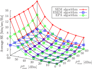
(a) Surface plots of the achievable SE when using the SEM, ESEM and RG-EPA algorithms.

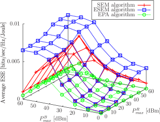
(b) Surface plots of the achievable ESE when using the SEM, ESEM and RG-EPA algorithms.

Figure 5: The average achievable SE and ESE of the SEM, ESEM and RG-EPA algorithms upon varying $P_{max}^{B}$ and $P_{max}^{R}$. The parameters in Table I with $N=6$, $K=10$, $M=2$, $\alpha=0.1$ and a cell radius of $1.75$km are used.

As shown in Fig. 5(a), the achievable SE is monotonically increasing with $P_{max}^{B}$ and $P_{max}^{R}$ when using the SEM algorithm. This is not unexpected, since the SEM algorithm optimally allocates all the available power for the sake of achieving the maximum SE. By comparison, we observed from Fig. 5(a) and Fig. 5(b) that both the achievable SE and ESE of the ESEM algorithm saturate at some moderate values of $P_{max}^{B}$ and/or $P_{max}^{R}$. This is because the ESEM algorithm only allocates “just” enough power (that may be lower than the power budget values of $P_{max}^{B}$ and/or $P_{max}^{R}$) for the sake of achieving the maximum ESE. On the other hand, the ESE performance of the SEM algorithm is severely degraded upon further increasing $P_{max}^{B}$ and/or $P_{max}^{R}$ after its ESE performance reaches the peak, as shown in Fig. 5(b). This is because the ESE metric is a quasiconcave function of the transmit powers – its numerator (i.e. the SE) increases logarithmically with the transmit powers, while its denominator increases linearly with the transmit powers. In fact, the peak ESE of the SEM algorithm is attained at $P_{max}^{B}=40$dBm and $P_{max}^{R}=40$dBm, as seen in Fig. 5(b), and the associated normalized optimality gap is only $-0.074$. By contrast, the achievable ESE when using the ESEM algorithm also saturates at around $P_{max}^{B}=40$dBm and $P_{max}^{R}=40$dBm. Thus, the operating point of “$P_{max}^{B}=40$dBm and $P_{max}^{R}=40$dBm” may strike an attractive balance between SEM and ESEM. Of course, the required trade-off may be struck on a case-by-case basis in practical systems.

Additionally, the RG-EPA algorithm performs significantly worse in terms of SE when compared to the SEM algorithm, and in terms of ESE when compared to the ESEM algorithm. Furthermore, the RG-EPA algorithm performs even worse than the SEM algorithm in terms of ESE. Although the obtained SE when using the RG-EPA algorithm is, in some cases, higher than the SE obtained when using the ESE algorithm, this performance improvement comes at a great cost to the ESE performance of the RG-EPA algorithm.

Finally, note that although both the SE of the SEM algorithm, and the ESE of the ESEM algorithm are non-decreasing as either $P_{max}^{B}$ or $P_{max}^{R}$ is increased, the effect of increasing $P_{max}^{B}$ on the SE or ESE is significantly more pronounced, than that of applying the same increase to $P_{max}^{R}$. The intuitive reasoning behind this is that the power available at the BS has a more pronounced effect on the system’s performance, since the direct links and, more importantly, the BS-to-RN links rely on the BS. Therefore, increasing $P_{max}^{R}$ is futile if the BS-to-RN links are not allocated sufficient power to support the RN-to-UE links.

VI-C The achievable SE and ESE as a function of $M$ and the cell radius

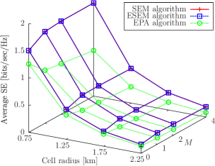
(a) Surface plots of the achievable SE when using the SEM, ESEM and RG-EPA algorithms.

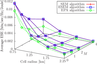
(b) Surface plots of the achievable ESE when using the SEM, ESEM and RG-EPA algorithms.

Figure 6: The average achievable SE and ESE of the SEM, ESEM and RG-EPA algorithms upon varying $M$ and cell radius, and using the parameters in Table I with $N=6$, $K=10$, $\alpha=0.1$, $P_{max}^{B}=20$dBm and $P_{max}^{R}=10$dBm.

Fig. 6 illustrates some advantages and disadvantages of employing RNs in the cellular system considered. We observe that the specific low values of the power constraints result in the same solutions for both the SEM and ESEM algorithms. This phenomenon was also shown in Fig. 5.

As evidenced in Fig. 6(a), the attainable SE increases with $M$, which is a benefit of the additional selection diversity, when forming relaying links. However, the attainable SE does not increase substantially beyond $M=2$. In fact, only an increase of $0.1\%$ is attained for the SE when $M$ is increased from $2$ to $4$ at a cell radius of $0.75$km. On the other hand, the cost in terms of ESE is significant ($36.4\%$), as shown in Fig. 6(b). This suggests that employing RNs does not constitute an energy-spectral-efficient technique although it increases the SE of a cellular system, which is partially due to the power amplifier inefficiency and owing to the non-negligible fixed circuit energy dissipation. Note furthermore that both the attainable SE and ESE are decreasing upon increasing the cell radius as a result of the increased path-loss of all the wireless links. However, this reduction is relatively small between a cell radius of $1.75$km and $2.25$km. The reason behind this phenomenon is that both the SEM and ESEM algorithms will selectively serve the UEs nearer to the BS, so that a similar performance may be attained without suffering from a substantial path-loss. This is also the reason why the gain in SE gleaned by employing RNs at a cell radius of $2.25$km seems negligible in Fig. 6(a). Once again, the RG-EPA algorithm performs worse both in terms of SE and ESE performance.

VI-D The achievable SE and ESE as a function of $N$ and $N_{B}$

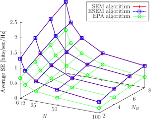
(a) Surface plots of the achievable SE when using the SEM, ESEM and RG-EPA algorithms.

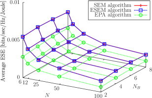
(b) Surface plots of the achievable ESE when using the SEM, ESEM and RG-EPA algorithms.

Figure 7: The average achievable SE and ESE of the SEM, ESEM and RG-EPA algorithms upon varying $N$ and $N_{B}$, and using the parameters in Table I with $M=2$, $K=10$, $\alpha=0.1$, $P_{max}^{B}=20$dBm, $P_{max}^{R}=10$dBm and a cell radius of $0.75$km.

Fig. 7 illustrates the effect of increasing $N$ and $N_{B}$ on the attainable SE and ESE. Note that in a similar fashion to Fig. 6, the SEM and ESEM algorithms attain the same solutions in the operating region considered.

Observe from both Figs. 7(a) and 7(b) that the attainable SE and ESE increase upon increasing $N_{B}$. This is due to the increased attainable spatial degrees of freedom at the BS in the first transmission phase, which allows for more direct transmissions overall. However, both the SE and ESE are reduced upon increasing $N$, which suggests that increasing the number of subcarrier blocks does not increase the average efficiency of each block. This is because the power constraints are fixed and thus there is insufficient power for fully exploiting the additional subcarrier blocks. However, note that both total SE and ESE do indeed increase upon increasing $N$, which may be explicitly seen upon multiplying the results of Figs. 7(a) and 7(b) by $NW$. The RG-EPA algorithm performs worse in both cases as expected.

VII Conclusions and future work

In this paper, firstly a novel transmission protocol based on joint transmit-BF and receive-BF was developed for the multi-relay MIMO-OFDMA cellular network considered. This protocol allows for achieving high-SE performance for the MIMO broadcast network consisting of a BS, multiple RNs and multiple UEs. The associated MIMO channel matrices were mathematically decomposed into multiple MISO channels, which we referred to as SMCs, using receive-BF. By applying ZFBF at the transmitter, the interference between SMC-based concurrent transmissions is completely eliminated, provided that perfect CSI-knowledge is available. For the purposes of obtaining a higher multiplexing gain, the SMCs may be grouped according to the semi-orthogonality criterion. Consequently, a pair of grouping algorithms were proposed, referred to as ESGA and OCGA. The former exhaustively enumerates all of the possible groupings, whereas the latter aims to be a lower-complexity design alternative. Finding the SE-optimal and ESE-optimal SMC groupings as well as their associated optimal power control variables were formulated as optimization problems. With the aid of several variable relaxations and transformations, these optimization problems were transformed into concave optimization problems. Thus, the dual decomposition approach was employed for finding the optimal solutions. We demonstrated that the OCGA constitutes an attractive alternative to ESGA, since it offers a near-optimal performance at a substantially reduced complexity. Furthermore, several numerical results were presented for characterizing the system’s attainable SE and ESE performance across a wide range of system parameters, such as the transmit power constraints, cell radius, the number of RNs, the number of BS antennas and the number of subcarrier blocks. Additionally, we demonstrated that our SEM/ESEM algorithms perform significantly better than the benchmark RG-EPA algorithm.

In our future work, we will consider unity frequency reuse multi-relay multi-cell networks. Thus, these networks are interference-limited, rather than noise-limited. Consequently, improved transmission protocols and optimization methods are required for managing both the intra-cell and inter-cell interference in order to improve the system’s SE and ESE performance.

References

- [1] M. Salem, A. Adinoyi, M. Rahman, H. Yanikomeroglu, D. Falconer, Y.-D. Kim, E. Kim, and Y.-C. Cheong, “An overview of radio resource management in relay-enhanced OFDMA-based networks,” IEEE Communications Surveys Tutorials, vol. 12, no. 3, pp. 422–438, Apr. 2010.
- [2] L. Hanzo, Y. Akhtman, L. Wang, and M. Jiang, MIMO-OFDM for LTE, WIFI and WIMAX: Coherent Versus Non-Coherent and Cooperative Turbo-Transceivers. Wiley-IEEE Press, 2010.
- [3] C. Han, T. Harrold, S. Armour, I. Krikidis, S. Videv, P. Grant, H. Haas, J. Thompson, I. Ku, C.-X. Wang, T. A. Le, M. Nakhai, J. Zhang, and L. Hanzo, “Green radio: radio techniques to enable energy-efficient wireless networks,” IEEE Communications Magazine, vol. 49, no. 6, pp. 46–54, Jun. 2011.
- [4] G. Caire and S. Shamai, “On the achievable throughput of a multiantenna Gaussian broadcast channel,” IEEE Transactions on Information Theory, vol. 49, no. 7, pp. 1691–1706, Jul. 2003.
- [5] S. Vishwanath, N. Jindal, and A. Goldsmith, “Duality, achievable rates, and sum-rate capacity of Gaussian MIMO broadcast channels,” IEEE Transactions on Information Theory, vol. 49, no. 10, pp. 2658–2668, Oct. 2003.
- [6] M. H. M. Costa, “Writing on dirty paper,” IEEE Transactions on Information Theory, vol. 29, no. 3, pp. 439–441, May 1983.
- [7] T. Yoo and A. Goldsmith, “On the optimality of multiantenna broadcast scheduling using zero-forcing beamforming,” IEEE Journal on Selected Areas in Communications, vol. 24, no. 3, pp. 528–541, Mar. 2006.
- [8] N. Ul Hassan and M. Assaad, “Low complexity margin adaptive resource allocation in downlink MIMO-OFDMA system,” IEEE Transactions on Wireless Communications, vol. 8, no. 7, pp. 3365–3371, Jul. 2009.
- [9] G. Raleigh and J. Cioffi, “Spatio-temporal coding for wireless communication,” IEEE Transactions on Communications, vol. 46, no. 3, pp. 357–366, Mar. 1998.
- [10] K.-K. Wong, R. Murch, and K. Letaief, “A joint-channel diagonalization for multiuser MIMO antenna systems,” IEEE Transactions on Wireless Communications, vol. 2, no. 4, pp. 773–786, Jul. 2003.
- [11] W. Ho and Y.-C. Liang, “Optimal resource allocation for multiuser MIMO-OFDM systems with user rate constraints,” IEEE Transactions on Vehicular Technology, vol. 58, no. 3, pp. 1190–1203, Mar. 2009.
- [12] M. Sharif and B. Hassibi, “On the capacity of MIMO broadcast channels with partial side information,” IEEE Transactions on Information Theory, vol. 51, no. 2, pp. 506–522, Feb. 2005.
- [13] A. Goldsmith, Wireless Communications. Cambridge University Press, New York, NY, USA, 2005.
- [14] D. Ng, E. Lo, and R. Schober, “Energy-efficient resource allocation in multi-cell OFDMA systems with limited backhaul capacity,” IEEE Transactions on Wireless Communications, vol. 11, no. 10, pp. 3618–3631, Oct. 2012.
- [15] G. Miao, N. Himayat, and G. Li, “Energy-efficient link adaptation in frequency-selective channels,” IEEE Transactions on Communications, vol. 58, no. 2, pp. 545 –554, Feb. 2010.
- [16] G. Miao, N. Himayat, G. Li, and S. Talwar, “Low-complexity energy-efficient scheduling for uplink OFDMA,” IEEE Transactions on Communications, vol. 60, no. 1, pp. 112–120, Jan. 2012.
- [17] K. T. K. Cheung, S. Yang, and L. Hanzo, “Achieving maximum energy-efficiency in multi-relay OFDMA cellular networks: A fractional programming approach,” IEEE Transactions on Communications, vol. 61, no. 7, pp. 2746–2757, Jul. 2013.
- [18] Z. Shen, R. Chen, J. Andrews, R. Heath, and B. Evans, “Low complexity user selection algorithms for multiuser MIMO systems with block diagonalization,” IEEE Transactions on Signal Processing, vol. 54, no. 9, pp. 3658–3663, Sept. 2006.
- [19] W. Yu and T. Lan, “Transmitter optimization for the multi-antenna downlink with per-antenna power constraints,” IEEE Transactions on Signal Processing, vol. 55, no. 6, pp. 2646–2660, Jun. 2007.
- [20] E. Lo, P. Chan, V. K. N. Lau, R. Cheng, K. Letaief, R. Murch, and W.-H. Mow, “Adaptive resource allocation and capacity comparison of downlink multiuser MIMO-MC-CDMA and MIMO-OFDMA,” IEEE Transactions on Wireless Communications, vol. 6, no. 3, pp. 1083–1093, Mar. 2007.
- [21] D. Ng, E. Lo, and R. Schober, “Dynamic resource allocation in MIMO-OFDMA systems with full-duplex and hybrid relaying,” IEEE Transactions on Communications, vol. 60, no. 5, pp. 1291–1304, May 2012.
- [22] G. Brante, I. Stupia, R. D. Souza, and L. Vandendorpe, “Outage probability and energy efficiency of cooperative MIMO with antenna selection,” IEEE Transactions on Wireless Communications, vol. 12, no. 11, pp. 5896–5907, Nov. 2013.
- [23] A. Zappone, P. Cao, and E. Jorswieck, “Energy efficiency optimization in relay-assisted MIMO systems with perfect and statistical CSI,” IEEE Transactions on Signal Processing, vol. 62, no. 2, pp. 443–457, Jan. 2014.
- [24] M. Avriel, W. E. Diewert, S. Schaible, and I. Zang, Generalized Concavity. Plenum Press, New York, NY, USA, 1988.
- [25] R. Devarajan, S. Jha, U. Phuyal, and V. Bhargava, “Energy-aware resource allocation for cooperative cellular network using multi-objective optimization approach,” IEEE Transactions on Wireless Communications, vol. 11, no. 5, pp. 1797–1807, May 2012.
- [26] W. Dinkelbach, “On nonlinear fractional programming,” Management Science, vol. 13, pp. 492–498, Mar. 1967.
- [27] D. Ng, E. Lo, and R. Schober, “Energy-efficient resource allocation for secure OFDMA systems,” IEEE Transactions on Vehicular Technology, vol. 61, no. 6, pp. 2572–2585, Jul. 2012.
- [28] C. Isheden, Z. Chong, E. Jorswieck, and G. Fettweis, “Framework for link-level energy efficiency optimization with informed transmitter,” IEEE Transactions on Wireless Communications, vol. 11, no. 8, pp. 2946–2957, Aug. 2012.
- [29] J. Laneman, D. Tse, and G. Wornell, “Cooperative diversity in wireless networks: Efficient protocols and outage behavior,” IEEE Transactions on Information Theory, vol. 50, no. 12, pp. 3062–3080, Dec. 2004.
- [30] 3GPP, “TR 36.814 V9.0.0: further advancements for E-UTRA, physical layer aspects (release 9),” Mar. 2010.
- [31] S.-J. Kim, A. Magnani, A. Mutapcic, S. Boyd, and Z.-Q. Luo, “Robust beamforming via worst-case SINR maximization,” IEEE Transactions on Signal Processing, vol. 56, no. 4, pp. 1539–1547, Apr. 2008.
- [32] S. Boyd and L. Vandenberghe, Convex Optimization. Cambridge University Press, New York, NY, USA, 2004.
- [33] L. Hanzo, O. Alamri, M. El-Hajjar, and N. Wu, Near-Capacity Multi-Functional MIMO Systems: Sphere-Packing, Iterative Detection and Cooperation. Wiley-IEEE Press, 2009.
- [34] A. Yeredor, “Non-orthogonal joint diagonalization in the least-squares sense with application in blind source separation,” IEEE Transactions on Signal Processing, vol. 50, no. 7, pp. 1545–1553, Jul. 2002.
- [35] P. Comon and C. Jutten, Handbook of Blind Source Separation: Independent Component Analysis and Applications. Academic Press, 2010.
- [36] G. Auer, O. Blume, V. Giannini, I. Godor, M. A. Imran, Y. Jading, E. Katranaras, M. Olsson, D. Sabella, P. Skillermark, and W. Wajda, “D2.3: Energy efficiency analysis of the reference systems, areas of improvements and target breakdown,” INFSO-ICT-247733 EARTH (Energy Aware Radio and NeTwork TecHnologies), Technical Report, Nov. 2010. [Online]. Available: https://bscw.ict-earth.eu/pub/bscw.cgi/d71252/EARTH_WP2_D2.3_v2.pdf
- [37] D. P. Bertsekas, Nonlinear Programming. Athena Scientific, Belmont, MA, USA, 1999.
- [38] W. Yu and R. Lui, “Dual methods for nonconvex spectrum optimization of multicarrier systems,” IEEE Transactions on Communications, vol. 54, no. 7, pp. 1310–1322, Jul. 2006.
- [39] K. Seong, M. Mohseni, and J. Cioffi, “Optimal resource allocation for OFDMA downlink systems,” in Proceedings of the IEEE International Symposium on Information Theory (ISIT’06), Seattle, Washington, USA, Jul. 2006, pp. 1394–1398.
- [40] D. Ng and R. Schober, “Cross-layer scheduling for OFDMA amplify-and-forward relay networks,” IEEE Transactions on Vehicular Technology, vol. 59, no. 3, pp. 1443–1458, Mar. 2010.
- [41] D. Palomar and M. Chiang, “A tutorial on decomposition methods for network utility maximization,” IEEE Journal on Selected Areas in Communications, vol. 24, no. 8, pp. 1439–1451, Aug. 2006.
- [42] O. Arnold, F. Richter, G. Fettweis, and O. Blume, “Power consumption modeling of different base station types in heterogeneous cellular networks,” in Proceedings of the Future Network and Mobile Summit, Florence, Italy, Jun. 2010.