A self-consistent Hartree-Fock approach for interacting bosons in optical lattices

Abstract

A theoretical study of interacting bosons in a periodic optical lattice is presented. Instead of the commonly used tight-binding approach (applicable near the Mott insulating regime of the phase diagram), the present work starts from the exact single-particle states of bosons in a cubic optical lattice, satisfying the Mathieu equation, an approach that can be particularly useful at large boson fillings. The effects of short-range interactions are incorporated using a self-consistent Hartree-Fock approximation, and predictions for experimental observables such as the superfluid transition temperature, condensate fraction, and boson momentum distribution are presented.

I Introduction

Ultracold atoms in optical lattices have recently emerged as a novel setting for physicists to study interacting many-body systems rmp:bloch ; review:Lewenstein . Usually made by a set of standing waves that are formed by interfering counter-propagating laser beams, optical lattices mimic the crystalline lattice potential in condensed matter systems.

The single particle potential for bosons in an optical lattice can be taken to be a cosine function of position in each orthogonal direction. At sufficiently low temperatures, and for sufficiently large optical lattice amplitude $V_{0}$, one can approximate such a system by an effective boson Hubbard model (BHM), in which the minima of the single-particle potential correspond to sites of the Hubbard model prl:jaksch1998 . As first shown by Fisher et al. prb:fisher1989 , the boson Hubbard model exhibits, at integer filling, a quantum phase transition between the superfluid phase and an incompressible Mott insulating phase.

Starting with the pioneering work of Greiner et al. nat:greiner , numerous experiments have explored the properties of bosons in optical lattices that realize the BHM jlowtemp:kohl ; prl:spielman2007 ; prl:MunKetterle ; nat:chin ; natphys:trotzky ; njp:becker ; sci:endres2011 ; prl:marknageri ; sci:chin . The transition from the superfluid to the Mott phase occurs with increasing $U/J$, where $U$ and $J$ are the on-site repulsion and nearest-neighbor tunneling matrix elements, respectively, in the BHM. These phases are separated by a quantum critical point at which the BEC transition temperature ${T_{\rm c}}$ is suppressed to zero with increasing $U/J$. This suppression was observed experimentally by Trotzky et al. natphys:trotzky , who could control $U/J$ by tuning the optical lattice depth parameter $V_{0}$, quantitatively confirming the BHM picture for bosons at unit filling.

The purpose of the present work is to explore bosons in optical lattices via a different approach without making the simplification to the BHM Hamiltonian but, rather, by studying the full Hamiltonian for bosons in a periodic optical lattice potential with short-ranged interactions. One motivation for our study is the fact that even non-interacting bosons in a periodic optical lattice will exhibit a strong suppression of the BEC transition temperature ${T_{\rm c}}$ with increasing $V_{0}$ (although ${T_{\rm c}}$ will always be nonzero), that is essentially due to the increasing effective mass (or flattened single-particle bands) associated with a larger optical lattice amplitude. The question we pose, then, is to what extent the ${T_{\rm c}}$ suppression observed by Trotzky et al. could be understood within this simple effective mass picture.

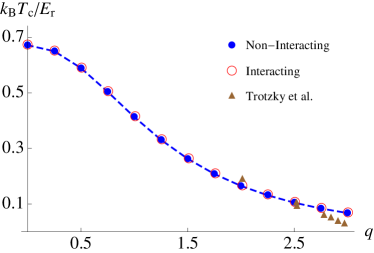
Figure 1: (Color online) We show in this plot the transition temperature ${T_{\rm c}}$, normalized to the recoil energy $E_{\rm r}$, as a function of the normalized optical lattice depth $q=V_{0}/4E_{\rm r}$, for bosons at unit filling in a periodic optical lattice potential. The blue points (and dashed curve) show the non-interacting case, the red circles show our interacting Hartree-Fock calculation, and the triangles show the experimental data from Ref. natphys:trotzky (indicated as “Trotzky et al.”). The latter shows a clear suppression for larger $q$ as the Mott insulating quantum critical point (at $q\simeq 3$ in this figure Capogrosso ) is approached

More generally, we are interested in understanding how interaction effects impact the observable properties of bosons in optical lattices far away from the regime where the BHM applies at low temperatures and large optical lattice depth. Our starting point is the problem of non-interacting bosons in a periodic potential. As we discuss below, the corresponding single-particle problem that we need to solve to describe this system is the one-dimensional Schrödinger equation for bosons in a cosine-shaped potential, also known as the Mathieu equation Abramowitz . We note that other recent theoretical works have explored the Mathieu equation in this context, including Zwerger Zwerger , who used the known bandwidth of the Mathieu equation to derive an approximation for the Hubbard tight-binding parameter, and McKay et al. pra:demarco , who studied the thermodynamics of trapped cold bosons using the Mathieu equation.

An additional question of interest, motivating our work, is how short range repulsive interactions (characterized by scattering length $a_{s}>0$ or BHM repulsion $U>0$) impact observable properties of bosons such as ${T_{\rm c}}$. For large optical lattice depth and low filling, where the BHM applies, increasing the strength of repulsive interactions suppresses ${T_{\rm c}}$ as the Mott phase is approached. In contrast, for a uniform BEC (equivalent to our system at optical lattice depth $V_{0}=0$), increasing the repulsive interactions leads to an increase of ${T_{\rm c}}$ Baym99 ; rmp:andersen . To investigate this, we incorporate interactions for bosons in a periodic optical lattice within a self-consistent Hartree-Fock approximation. While Hartree-Fock is known to have a vanishing affect on ${T_{\rm c}}$ for a uniform gas, we find a small ${T_{\rm c}}$ enhancement for increasing $a_{s}$ for bosons in a periodic optical lattice.

Before proceeding to the details of our calculations, we first present our main results. In Fig. 1 we show $k_{\rm B}{T_{\rm c}}$ (with $k_{\rm B}$ the Boltzmann constant) for a non-interacting BEC in a periodic optical lattice, normalized to the recoil energy $E_{\rm r}=\frac{\hbar^{2}k^{2}}{2m}$, as a function of optical lattice depth $V_{0}$ in the combination $q\equiv V_{0}/4E_{\rm r}$, along with the results of the Trotzky et al. experiment and also our interacting Hartree-Fock approach (using the same parameters as the Trotzky et al. experiment). Incorporating the Trotzky et al. results into this figure required expressing the data of Ref. natphys:trotzky in terms of the parameters $V_{0}/4E_{\rm r}$ via an approximate tight-binding formula for the hopping matrix element $J$, as described below. However, this plot shows that the Trotzky et al. ${T_{\rm c}}$ data quantitatively agrees with the non-interacting theory for small optical lattice depth, and shows a clear suppression for larger optical lattice depth as the Mott insulating quantum critical point is approached.

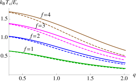
Figure 2: (Color online) The top panel shows ${T_{\rm c}}$ vs. normalized optical lattice depth $q$ for parameters consistent with the Trotzky et al. experiment, but including larger filling values ($f=N/N_{\rm sites}$ with $N$ the particle number and $N_{\rm sites}$ the number of lattice sites). For each case, the solid curve is the interacting case and the dashed curve is the non-interacting case. Although these curves show a slight separation of the non-interacting and interacting curves with increasing filling $f$, the difference is quite small even for the largest filling. In the bottom panel we plot ${T_{\rm c}}$ vs. $q$ for larger $a_{s}$ ($a_{s}/a=0.1$), which shows a significant enhancement of ${T_{\rm c}}$ due to interactions.

Figure 1 also shows that our interacting Hartree-Fock approach is indistinguishable from non-interacting bosons in an optical lattice in this parameter regime (although our interacting ${T_{\rm c}}$ is slightly higher than the non-interacting case). In Fig. 2, we show our results for various filling values at small scattering length (top panel, $a_{s}$ consistent with parameters of Ref. natphys:trotzky ) and for large scattering length (bottom panel $a_{s}/a=0.1$, with $a$ the optical lattice spacing, but other parameters still consistent with Ref. natphys:trotzky ), with only the latter showing a significant enhancement of the transition temperature arising from the repulsive interactions.

Our work can be summarized as the following: we construct the wave functions for bosons in an optical lattice using Mathieu Functions, and obtain the single particle energies from the eigenvalues of Mathieu equation. We are then able to calculate experimental observables for bosons in an optical lattice and verify their agreement with experiments. Within our Hartree-Fock self-consistent scheme, we find that interaction raises the critical temperature, makes more atoms condense, and results in a more uniform boson density. The finite size effect and boundary conditions are also considered in our calculation.

We organize this paper as follows. In Sec. II we will introduce the Mathieu equation which naturally describes the single-particle states of non-interacting bosons in an optical lattice, with the transition temperature and number equations depending on the Mathieu equation eigenvalues. In Sec. III, we describe our method for incorporating interaction effects using a self-consistent Hartree-Fock approach that leads to coupled equations that must be solved numerically. In Sec. IV we present our results from solving these equations, and describe how repulsive interactions modify observables like the superfluid transition temperature, condensate fraction, local boson density and boson momentum distribution. In this section, we initially choose system parameters consistent with the experiments of Trotzky et al. natphys:trotzky before subsequently considering the effect of larger filling and larger scattering length. Section V concludes the paper and provides some additional discussion.

II System Hamiltonian and non-interacting limit

Our model Hamiltonian $H=H_{0}+H_{1}$ for bosons in an optical lattice consists of a single particle ($H_{0}$) and interaction ($H_{1}$) piece:

$$H_{0} = \int d^{3}r\,\Phi^{\dagger}({\bf r})\Big{[}-\frac{\hbar^{2}\nabla^{2}}{2m}-\mu+V({\bf r})\Big{]}\Phi({\bf r}),$$ (1)

$$H_{1} = \frac{g}{2}\int d^{3}r\,\Phi^{\dagger}({\bf r})\Phi^{\dagger}({\bf r})\Phi({\bf r})\Phi({\bf r}),$$ (2)

where $\Phi({\bf r})$ is a bosonic field operator satisfying $[\Phi({\bf r}),\Phi^{\dagger}({\bf r}^{\prime})]=\delta^{(3)}({\bf r}-{\bf r}^{\prime})$, $m$ is the boson mass, and $\hbar$ is Planck’s constant. Here, $g=\frac{4\pi\hbar^{2}a_{s}}{m}$ with $a_{s}$ the s-wave scattering length, and $V({\bf r})=V_{0}(\cos^{2}{kx}+\cos^{2}{ky}+\cos^{2}{kz}-\frac{3}{2})$ is the imposed optical lattice potential characterized by the optical lattice depth $V_{0}$ and the wavevector $k$ (with the lattice spacing $a=\pi/k$). The subtracted constant 3/2 ensures the spatial integration of $V({\bf r})$ vanishes.

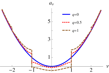
Figure 3: (Color Online) The Mathieu characteristic function for the even Mathieu function gives the dispersion, i.e. $a_{\nu}=\varepsilon_{\nu}/E_{\rm r}$. Here $q=V_{0}/4E_{\rm r}=1$, $0.5$, $0$. The ground state energy (the bottom of the curves) is lowered as the optical lattice potential $V_{0}$ increases. The Characteristic Function is reduced to a parabola when $V_{0}=0$.

In the absence of interactions, $g=0$, $H$ is solvable by considering the eigenfunctions of the single-particle Hamiltonian $\hat{h}\equiv-\frac{\nabla^{2}}{2m}+V({\bf r})$, (henceforth we take $\hbar=1$) that satisfy

$$\hat{h}\Phi_{\mbox{\boldmath$\nu$}}({\bf r})=E_{\mbox{\boldmath$\nu$}}\Phi_{\mbox{\boldmath$\nu$}}({\bf r}),$$ (3)

where $\mbox{\boldmath$\nu$}=(\nu_{x},\nu_{y},\nu_{z})$ is the eigenvalue index, $E_{\mbox{\boldmath$\nu$}}$ is the total energy, and $\Phi_{\mbox{\boldmath$\nu$}}({\bf r})$ is the 3D wave function. We can write $\Phi_{\mbox{\boldmath$\nu$}}({\bf r})$ as a product of wave functions in the $x$, $y$, and $z$ directions as $\Phi_{\mbox{\boldmath$\nu$}}({\bf r})=\phi_{\nu_{x}}(x)\phi_{\nu_{y}}(y)\phi_{\nu_{z}}(z)$, with each of the $\phi_{\nu_{i}}$ satisfying a corresponding 1D Schrödinger equation with a 1D potential:

$$\left[-\frac{1}{2m}\frac{d^{2}}{dx^{2}}+V_{0}\left(\cos^{2}{kx}-\frac{1}{2}\right)\right]\phi_{\nu}(x)=\varepsilon_{\nu}\phi_{\nu}(x),$$ (4)

with 1D eigenvalue $\varepsilon_{\nu}$. This can furthermore be rearranged into the form of the Mathieu equation Abramowitz :

$$\frac{d^{2}\phi_{\nu}(u)}{du^{2}}+(a_{\nu}-2q\cos{2u})\phi_{\nu}(u)=0,$$ (5)

where $u=kx$ is a dimensionless coordinate. Here, $a_{\nu}=\frac{\varepsilon_{\nu}}{E_{\rm r}}$ and $q=\frac{V_{0}}{4E_{\rm r}}$ are dimensionless forms of the 1D eigenvalue and optical lattice depth, normalized to the recoil energy $E_{\rm r}=\frac{k^{2}}{2m}$. The Mathieu Equation (Eq. 5) has even and odd periodic solutions, $ce(a_{\nu},q,u)$ and $se(b_{\nu},q,u)$, respectively, with $a_{\nu}$ and $b_{\nu}$ called the Mathieu characteristic functions (playing the role of the eigenvalue here) for the even and odd solutions. The real number $\nu$ determines the periodicity of the solutions, and generally $a_{\nu}=b_{\nu}$ except when $\nu$ is an integer. In Fig. 3, we plot $a_{\nu}(q)$ as a function of $\nu$ for three values of the normalized optical lattice depth, $q=0,~{}0.5,~{}1$, showing a typical band structure for particles in a periodic potential, with $\nu=1$ being the Brillouin zone boundary.

The Mathieu equations solutions $ce(a_{\nu},q,u)$ and $se(b_{\nu},q,u)$, analogous to cosine and sine, respectively, can also be combined into analogues of complex exponential functions as:

$$me_{\nu}(u,q)=ce(a_{\nu},q,u)+i\,se(b_{\nu},q,u),$$ (6)

which satisfy a Bloch theorem:

$$me_{\nu}(u+n\pi,q)={\rm e}^{in\pi\nu}me_{\nu}(u,q).$$ (7)

Here, $n$ is any integer, so that $\nu$ can be regarded as a Bloch quasi-momentum, with $p=\pi\nu/a$.

To study the BEC, we consider a box of volume $V=L^{3}$ that encloses $N_{\rm s}$ lattice sites along each direction, with $N_{\rm sites}=N_{\rm s}^{3}$ being the total number of lattice sites in the cubic lattice. Imposing periodic boundary conditions implies, for our 1D solutions, $\phi_{\nu}(k[x+L])=\phi_{\nu}(kx)$. Using Eq. (7) with $n\pi=kL=\pi N_{\rm s}$, we have

$$me_{\nu}(u+kL,q)={\rm e}^{i\pi\nu N_{s}}me_{\nu}(u,q),$$ (8)

which implies the $\nu$ satisfy $\nu_{m}=2m/N_{\rm s}$ with $m$ any integer, to have the phase on the right side be unity. Therefore, our quantized wave functions for bosons in an optical lattice with periodic boundary conditions can be written as

$$\phi_{\nu_{n}}(x)=\begin{cases}\frac{1}{\sqrt{L}}me_{\nu_{n}}\Big{(}kx,q\Big{)},&\text{if $n\neq 0$ },\cr\sqrt{\frac{2}{L}}ce\Big{(}a_{0},q,kx\Big{)},&\text{if $n=0$ },\end{cases}$$ (9)

where the special case of $n=0$ occurs because the odd Mathieu function is not defined for $\nu=0$. With this definition, the $\phi_{\nu_{n}}(x)$ satisfy the normalization

$$\int_{0}^{L}dx\phi_{\nu_{n}}^{*}(x)\phi_{\nu_{m}}(x)=\delta_{mn}.$$ (10)

The particle number equation used to determine the BEC transition temperature ${T_{\rm c}}$ and condensate fraction below ${T_{\rm c}}$ is

$$N=N_{0}+\sum_{{\bf n}\neq 0}n_{\rm B}\big{(}E_{{\bf n}}-\mu\big{)},$$ (11)

with $N$ the total particle number, $N_{0}$ the number in the lowest state $\Phi_{\bf 0}({\bf r})=\phi_{0}(x)\phi_{0}(y)\phi_{0}(z)$, and $E_{\bf n}=E_{\rm r}(a_{\nu_{x}}+a_{\nu_{y}}+a_{\nu_{z}})$. The sum in Eq. (11) is understood to be over integers $n_{x}$, $n_{y}$, and $n_{z}$ from $-\infty$ to $\infty$. Approximating the sum by an integral by introducing the continuous variable $\nu_{x}=2n_{x}/N_{\rm s}$ (and similarly for $\nu_{y}$ and $\nu_{z}$), we have

$$N = N_{0}+\frac{N_{\rm s}^{3}}{8}\int_{-\infty}^{\infty}d^{3}\nu\,n_{\rm B}\big{(}E_{\mbox{\boldmath$\nu$}}-\mu\big{)},$$ (12)

$$= N_{0}+N_{\rm sites}\int_{0}^{\infty}d^{3}\nu\,n_{\rm B}\big{(}E_{\mbox{\boldmath$\nu$}}-\mu\big{)},$$

where in the second line we used the symmetry of the integrand under $\mbox{\boldmath$\nu$}\to-\mbox{\boldmath$\nu$}$ to simplify the integrals and introduced $N_{\rm sites}=N_{\rm s}^{3}$, the total number of lattice sites in our system.

We can then solve for the superfluid transition temperature ${T_{\rm c}}$ from Eq. (11), which occurs when the chemical potential reaches the lowest state, i.e. $\mu/E_{\rm r}=3a_{0}(q)$, with $a_{0}(q)$ referring to the characteristic function’s minimum at $\nu=0$. As usual for a BEC, the condensate number below ${T_{\rm c}}$ is determined by Eq. (12) with $\mu$ pinned to the bottom of the band ($\mu=0$ for a free gas, but $\mu=E_{0}$ for the present case). Having established the notation of the Mathieu equation and reviewed the non-interacting BEC problem for this case, we now turn to the interacting case and present our self-consistent Hartree-Fock approach.

III Hartree-Fock Self-Consistent Scheme: Ansatz

In the preceding section, we studied non-interacting bosons in an optical lattice with the Mathieu equation. In this section, we try to capture interaction effects by using Hartree-Fock approximation. For bosons in a uniform potential, interaction effects vanish identically within the Hartree-Fock approximation Baym99 . This follows because, for a uniform gas, the Hartree-Fock contribution to interactions enter as a shift in the chemical potential $\mu\to\mu-2gn$ with $n$ the local density, and can therefore be absorbed in a redefinition of the chemical potential.

In the presence of an optical lattice potential, this translational invariance is broken and physical properties such as the superfluid transition temperature can be modified by interaction effects, even within the Hartree-Fock approximation. This is seen most strikingly in the suppression of the transition temperature to $0\,{\rm K}$ for bosons at integer filling, resulting in a quantum phase transition to the Mott insulating state. Here our main interest is studying such interaction effects away from the Mott regime at low temperature and integer filling, using a self-consistent Hartree-Fock approach that utilizes the Mathieu function representation for bosons in an effective periodic potential.

Our self-consistent Hartree-Fock approximation is motivated by first noting that bosons in a periodic cosine-shaped potential will have a local density that is also periodic. Approximately, this density is given by a constant piece plus a spatially-modulated cosine-shaped piece. Within the simplest Hartree-Fock approximation, one makes the replacement, for $H_{1}$,

$$\int\!\!d^{3}r\Phi^{\dagger}({\bf r})\Phi^{\dagger}({\bf r})\Phi({\bf r})\Phi({\bf r})\!\!\! \to \!\!\!2\int\!\!d^{3}r\Phi^{\dagger}({\bf r})\Phi({\bf r})\langle\Phi^{\dagger}({\bf r})\Phi({\bf r})\rangle,$$ (13)

$$= 2\int d^{3}r\Phi^{\dagger}({\bf r})\Phi({\bf r})n({\bf r}),$$

with the $2$ coming from the two ways such a contraction can occur, so that a spatially-periodic boson density $n({\bf r})$ acts like an additional single-particle potential $\propto gn({\bf r})$ on the bosons.

Although Eq. (13) contains the essential physics of our scheme, we now derive it via a more formal method. To do this we consider the single-particle Green’s function for bosons described by the Hamiltonian $H$:

$$G({\bf r}_{1},\tau_{1};{\bf r}_{2},\tau_{2})=-\langle T_{\tau}\Phi({\bf r}_{1},\tau_{1})\Phi^{\dagger}({\bf r}_{2},\tau_{2})\rangle,$$ (14)

where $\tau$ refers to imaginary time, $T_{\tau}$ is the imaginary time ordering operator, and the time dependence of $\Phi({\bf r},\tau)$ is determined by the Heisenberg equation of motion

$$\frac{\partial\Phi({\bf r},\tau)}{\partial\tau}=\big{[}H,\Phi({\bf r},\tau)\big{]}.$$ (15)

Because our system is translationally invariant in the time direction, $G({\bf r}_{1},\tau_{1};{\bf r}_{2},\tau_{2})$ can be taken to be a function only of $\tau_{1}-\tau_{2}$ and furthermore can be expressed in terms of a sum over bosonic Matsubara frequencies:

$$G({\bf r}_{1},\tau_{1};{\bf r}_{2},\tau_{2})=k_{\rm B}T\sum_{\omega}{\rm e}^{-i\omega(\tau_{1}-\tau_{2})}G({\bf r}_{1},{\bf r}_{2};\omega).$$ (16)

The Dyson equation for $G({\bf r},{\bf r}^{\prime};\omega)$ is:

$$G({\bf r},{\bf r}^{\prime};\omega)=G_{0}({\bf r},{\bf r}^{\prime};\omega)$$ (17)

$$+\int d^{3}r_{1}\,d^{3}r_{2}\,G_{0}({\bf r},{\bf r}_{1};\omega)\Sigma({\bf r}_{1},{\bf r}_{2};\omega)G({\bf r}_{2},{\bf r}^{\prime};\omega),$$

with $\hat{h}({\bf r})\equiv-\frac{\nabla^{2}}{2m}-\mu+V({\bf r})$. Here, $G_{0}({\bf r},{\bf r}^{\prime};\omega)$ is the bare Green’s function (for $H_{1}=0$) satisfying

$$\big{[}i\omega-\hat{h}({\bf r})\big{]}G_{0}({\bf r},{\bf r}^{\prime};\omega)=\delta({\bf r}-{\bf r}^{\prime}),$$ (18)

and $\Sigma({\bf r},{\bf r}^{\prime};\omega)$ is the self-energy which, within the Hartree-Fock approximation, has the form (as reviewed in Appendix A):

$$\Sigma({\bf r},{\bf r}^{\prime};\omega)=2gn({\bf r})\delta({\bf r}-{\bf r}^{\prime}).$$ (19)

Plugging this into Eq. (17), and acting on both sides with the operator $i\omega-\hat{h}({\bf r})$, we arrive at:

$$\big{[}i\omega-\hat{h}({\bf r})-2gn({\bf r})\big{]}G({\bf r},{\bf r}^{\prime};\omega)=\delta({\bf r}-{\bf r}^{\prime}),$$ (20)

equivalent to:

$$G^{-1}({\bf r},{\bf r}^{\prime};\omega)=i\omega-\Big{(}-\frac{\nabla^{2}}{2m}-\mu+V_{0}({\bf r})+2gn({\bf r})\Big{)}.$$ (21)

so that, indeed, the Green’s function within the Hartree-Fock approximation only depends on the effective potential $V_{0}({\bf r})+2gn({\bf r})$.

Since the boson density $n({\bf r})$ is highest at minima of $V_{0}({\bf r})$, and because $g>0$, the spatially-varying part of $n({\bf r})$ will tend to cancel out the imposed periodic potential, so that the bosons effectively “see” a lower lattice depth. As we shall see, this will tend to increase the transition temperature, and also make the BEC phase occurring below ${T_{\rm c}}$ more spatially uniform than predicted by a non-interacting theory.

To show this in detail, we proceed by making one additional approximation, by assuming that the boson density as a function of position can be taken to be a constant piece plus a piece that varies, spatially, in the same manner as the imposed optical lattice potential [i.e., according to the function $v({\bf r})$]:

$$n({\bf r})\approx\frac{f}{a^{3}}[1-cv({\bf r})],$$ (22)

with $f=N/N_{\rm sites}$ the filling, $v({\bf r})=\cos^{2}kx+\cos^{2}ky+\cos^{2}kz-\frac{3}{2}$ the function appearing in the definition of the optical lattice potential, and $c$ an unknown parameter to be determined self-consistently. The approximation Eq. (22) ensures $\int d^{3}r\,n({\bf r})=N$, since the integral of the spatially dependent term over the unit cell vanishes. Because $\left|v({\bf r})\right|<3/2$, for the density $n({\bf r})$ to be positive we need $-2/3<c<2/3$. Additionally, since we expect the boson density to reach maxima at the minima of the lattice, we must have $c>0$.

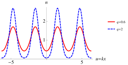
Figure 4: (Color online) Two calculated non-interacting boson densities are compared in this plot. Here the dashed blue and solid red curves are the modulus squared of the condensate wavefunction, $n=|\left|me(0,q,u)\right||^{2}$ for $q=2$ and $q=0.6$, respectively. When $q$ is small, the density resembles a cosine shape plus a constant. However, the $q=2$ curves show deviations from this.

Translational symmetry dictates that $n({\bf r})$ have the same periodicity as the lattice, so that $n({\bf r})$ has the same shape in each unit cell. However, Eq. (22) makes the additional assumption that the spatial variation of $n({\bf r})$ is of the same form as the imposed optical lattice, up to a scaling parameter, which is $c$. This assumption is valid at small optical lattice depth since the modulus squared of the Mathieu functions is indeed approximately given by a constant plus a cosine at small $q$, as follows from the expansion of Mathieu functions for small $q$ (Ref. web:nistmath ):

$$me(\nu,q,u)=e^{i\nu u}-\frac{q}{4}\Big{[}\frac{1}{\nu+1}e^{i(\nu+2)u}-\frac{1}{\nu-1}e^{i(\nu-2)u}\Big{]}$$

$$\qquad\qquad+{\cal O}(q^{2}),$$ (23)

where $me(\nu,q,u)=ce(a_{\nu},q,u)+ise(b_{\nu},q,u)$. This formula implies that if the normalized lattice depth $q$ is sufficiently small, the only terms that will contribute are the first line of Eq. (23). To illustrate this, in Fig. 4 we plot the modulus squared of the Mathieu functions for $q=0.6$ and $q=2$. While the $q=0.6$ curve is clearly given by a constant plus plus cosine piece, the $q=2$ curve exhibits deviations from this. In the following, we aim to use Eq. (22) beyond the small-$q$ regime. This amounts to assuming that the effect on interactions of the higher-order terms in Eq. (23) is small.

Within the preceding assumptions, the interacting Green’s function Eq. (21) can be written as a sum over eigenfunctions of an effective Mathieu equation eigenproblem with a modified single-particle potential:

$$G({\bf r},{\bf r}^{\prime};\omega)=\sum_{\mbox{\boldmath$\nu$}}\frac{\Phi_{\mbox{\boldmath$\nu$}}({\bf r})\Phi_{\mbox{\boldmath$\nu$}}({\bf r}^{\prime})}{i\omega-\epsilon_{\mbox{\boldmath$\nu$}}},$$ (24)

where the single-particle states $\Phi_{\mbox{\boldmath$\nu$}}({\bf r})$ now satisfy

$$\left[-\frac{\nabla^{2}}{2m}+\left(V_{0}-\frac{2gfc}{a^{3}}\right)v({\bf r})\right]\Phi_{\mbox{\boldmath$\nu$}}({\bf r})=E_{\mbox{\boldmath$\nu$}}\Phi_{\mbox{\boldmath$\nu$}}({\bf r}),$$ (25)

with $\epsilon_{\mbox{\boldmath$\nu$}}=E_{\mbox{\boldmath$\nu$}}+\frac{2gf}{a^{3}}$. Thus, the eigenvalue problem Eq. (25) is identical to the original eigenvalue problem Eq. (3) but with a modified effective optical lattice potential $V_{0}-\frac{2gfc}{a^{3}}$. This implies that the solutions to Eq. (25) are once again built from a product of three Mathieu functions but with the replacement $q\to\bar{q}$ with

$$\bar{q}=\frac{1}{4E_{\rm r}}\left[V_{0}-\frac{2gfc}{a^{3}}\right]=q-\frac{4}{\pi}\frac{a_{s}}{a}fc,$$ (26)

where in the second equality we used the relation $g=4\pi a_{s}/m$ between the coupling parameter and the boson $s$-wave scattering length $a_{s}$. Thus, as noted above, that interaction effects can be seen as canceling part of the optical lattice, since $\bar{q}<q$. The unknown parameter $c$ will be determined self-consistently by considering the thermodynamic equations of motion for our system.

III.0.1 At the transition temperature

We start by describing our self consistent scheme at the transition temperature ${T_{\rm c}}$. Since our system is effectively non-interacting within the Hartree-Fock approximation, the boson density at temperature $T\geq{T_{\rm c}}$ is:

$$n(\mathbf{r})=\sum_{\mbox{\boldmath$\nu$}}n_{\rm B}(E_{\mbox{\boldmath$\nu$}}-\mu+\frac{2gf}{a^{3}})\left|\Phi_{\mbox{\boldmath$\nu$}}(\mathbf{r})\right|^{2},$$ (27)

where $n_{\rm B}$ is the Bose function. For our ansatz to be sensible, Eq. (27) should be equal to Eq. (22). At ${T_{\rm c}}$, such an agreement implies

$$\sum_{\mbox{\boldmath$\nu$}}n_{\rm B}(E_{\mbox{\boldmath$\nu$}}-E_{0})\left|\Phi_{\mbox{\boldmath$\nu$}}(\mathbf{r})\right|^{2}=\frac{f}{a^{3}}[1-cv({\bf r})],$$ (28)

where on the left side we used that, at the transition temperature, the chemical potential $\mu$ reaches the bottom of the effective dispersion that is the argument of the Bose function in Eq. (27): $\mu=E_{0}+\frac{2gf}{a^{3}}$.

In the following, we only impose Eq. (28) in an average sense. To do this, we consider the spatial integration of Eq. (28) over a unit cell. The right hand side is $f$, since $v({\bf r})$ vanishes from spatial averaging. Converting the summation $\sum_{\mbox{\boldmath$\nu$}}$ into an integral on the left hand side, we arrive at

$$f=\frac{{N_{\rm s}}^{3}}{V}\int d^{3}\nu~{}\int_{\rm cell}d^{3}r\,n_{\rm B}(E_{\mbox{\boldmath$\nu$}}-E_{0})$$ (29)

$$\times\left|me({2\nu_{x}},\bar{q},kx)\right|^{2}\left|me({2\nu_{y}},\bar{q},ky)\right|^{2}\left|me({2\nu_{z}},\bar{q},kz)\right|^{2}.$$

Using the normalization of the Mathieu functions

$$\int_{0}^{\pi}du~{}\left|me(2\nu_{x},\bar{q},u)\right|^{2}=\pi$$ (30)

and ${N_{\rm s}}^{3}/V=a^{-3}$, Eq. (29) is reduced to

$$\int d^{3}\nu~{}n_{\rm B}(E_{\mbox{\boldmath$\nu$}}-E_{0})=f,$$ (31)

which ensures Eq. (28) holds, on average, in each unit cell.

Next, we demand that Eq. (28) holds for the leading non-uniformity of the local density in each unit cell. To do this, we multiply both sides of Eq. (28) by $v({\bf r})$ and integrate over unit cell, obtaining a second self-consistent condition:

$$\int_{\rm cell}d^{3}r~{}n({\bf r})v({\bf r})=-\frac{3}{8}cf.$$ (32)

The left side of this equation can be simplified by introducing the function

$$I(\nu,\bar{q})=\int_{0}^{1}d\ell\left|me({2\nu},\bar{q},\pi\ell)\right|^{2}\left(\cos^{2}{\pi\ell}-\frac{1}{2}\right),$$ (33)

leading to:

$$-\frac{3}{8}cf=\int d^{3}\nu~{}n_{\rm B}(E_{\mbox{\boldmath$\nu$}}-E_{0})\left[I(\nu_{x},\bar{q})+I(\nu_{y},\bar{q})+I(\nu_{z},\bar{q})\right].$$ (34)

From Eq. (34) and Eq. (26), the effective lattice depth $\bar{q}$ can be solved. Because the filling is known from the number equation Eq. (31), the parameter $c$ can also be obtained. From these results, the interaction effect on the system’s density profile is described. Next, we explain how the same scheme works for the non-superfluid phase above ${T_{\rm c}}$ and in the superfluid phase below ${T_{\rm c}}$.

III.0.2 Above the Transition Temperature

The effective lattice depth $\bar{q}$ and the parameter $c$ are temperature dependent, following from the fact that interaction effects depend on the density distribution which is temperature dependent. When the system is above ${T_{\rm c}}$, all particles in the system are thermal, and the chemical potential is no longer pinned at the bottom of the band. Therefore the self-consistent conditions are Eq. (31) and Eq. (34), with $E_{0}$ replaced by $\mu-\frac{2gf}{a^{3}}$.

To obtain $\bar{q}$ and $c$, we can first obtain the filling $f$ from Eq. (31) for the critical temperature, then solve for the chemical potential $\mu$ and $c$ from the self-consistent conditions for $T>{T_{\rm c}}$, which paves the way for us to describe the spatial and thermodynamical properties of this interacting system.

III.0.3 Below the Transition Temperature

When the system is below ${T_{\rm c}}$, our self-consistent formulas are very similar, except that some of the bosons are in the condensate, and the chemical potential is once again pinned to the bottom of the effective dispersion. We have for the density:

$$n(\mathbf{r})=N_{0}\left|\Phi_{0}({\bf r})\right|^{2}+\sum_{\mbox{\boldmath$\nu$}\neq 0}n_{\rm B}(E_{\mbox{\boldmath$\nu$}}-\mu+\frac{16}{\pi}\frac{a_{s}}{a}fE_{\rm r})\left|\Phi_{\mbox{\boldmath$\nu$}}(\mathbf{r})\right|^{2},$$ (35)

where $N_{0}$ is the number of condensed particles and $\Phi_{0}({\bf r})$ is the ground-state wave function (a product of Mathieu functions for the $x$, $y$, and $z$ directions).

Integrating each term in Eq. (35) over a unit cell, we have

$$f=\frac{N_{0}}{N_{\rm sites}}+\int d^{3}\nu~{}n_{\rm B}(E_{\mbox{\boldmath$\nu$}}-E_{0}),$$ (36)

the generalization of Eq. (31) below ${T_{\rm c}}$. Similarly, by multiplying each term in Eq. (35) by $v({\bf r})$ and integrating over the unit cell, we obtain:

$$\begin{split}-\frac{3}{8}cf&=N_{0}\int_{\rm cell}d^{3}r~{}\left|\Phi_{0}({\bf r})\right|^{2}v({\bf r})\\ &+\int d^{3}\nu~{}n_{\rm B}(E_{\mbox{\boldmath$\nu$}}-E_{0})[I(\nu_{x},\bar{q})+I(\nu_{y},\bar{q})+I(\nu_{z},\bar{q})].\end{split}$$ (37)

Using the definition of $\Phi_{0}({\bf r})$, we can rewrite the first term as $3\frac{N_{0}}{N_{\rm s}}I_{0}(\bar{q})$, where $I_{0}(\bar{q})\equiv 2\int_{0}^{1}d\ell\left|ce(a_{0},\bar{q},\ell)\right|^{2}(\cos^{2}\pi\ell-\frac{1}{2})$. Then, combining with Eqs. $\eqref{equ:EffectiveLatDepthHFConsis}$ and $\eqref{equ:fillingEqbelowTc}$, we are able to solve for $\bar{q}$ and $c$ for the interacting system below ${T_{\rm c}}$.

IV Results

In the previous section we described our Hartree-Fock self-consistent approach for interacting bosons in optical lattices, in which the effect of inter-atomic interactions amounts to an effective periodic potential that partially offsets the imposed optical lattice. In this section, we present our numerical solution of the resulting equations in several parameter regimes. We will be interested in the shift of the transition temperature due to repulsive interactions, an issue that has been pursued theoretically for decades in the case of a homogeneous boson gas, with contradicting results including both positive and negative ${T_{\rm c}}$ shifts rmp:andersen .

We find a small increase of ${T_{\rm c}}$ with increasing repulsion within the self-consistent Hartree-Fock approximation that we interpret, physically, as being due to a spatial homogenization of the local boson density (relative to the non-interacting case) that makes it more likely for bosons to exchange with their neighbors, enhancing ${T_{\rm c}}$. We also compute the condensate fraction below the transition temperature as well as additional observables, such as the local boson density in a unit cell and the boson momentum distribution (measurable via time of flight experiements), which reflect the predicted homogenization of the local boson density in an optical lattice.

IV.1 Low filling and small scattering length

We start with the case of ⁸⁷Rb atoms in an optical lattice with parameters consistent with the experiments of Trotzky et al. natphys:trotzky , before considering larger filling and larger scattering lengths in subsequent sections. Trotzky et al. natphys:trotzky observed a suppression of the transition temperature ${T_{\rm c}}$ for bosons at unit filling with increasing $U/J$ (with $U$ the on-site repulsion and $J$ the nearest neighbor hopping matrix element) that is quantitatively consistent with the presence of a quantum phase transition to the Mott insulating state at $U/J\simeq 29.3$ Capogrosso . Figure 5 of Ref. natphys:trotzky shows experimental results, plotted as $k_{\rm B}{T_{\rm c}}/J$ vs. $U/J$. To compare to our theoretical calculations, we converted these data to the dimensionless parameters of our theory, $k_{\rm B}{T_{\rm c}}/E_{\rm r}$ and $V_{0}/E_{\rm r}$, using the approximate formulas Zwerger ; rmp:bloch

$$J = \frac{4}{\sqrt{\pi}}E_{\rm r}\left(\frac{V_{0}}{E_{\rm r}}\right)^{3/4}\exp\left[-2\left(\frac{V_{0}}{E_{\rm r}}\right)^{1/2}\right],$$ (38)

$$U = \sqrt{\frac{8}{\pi}}ka_{s}E_{\rm r}\left(\frac{V_{0}}{E_{\rm r}}\right)^{3/4},$$ (39)

for the Bose Hubbard model parameters $J$ and $U$. These can be combined to give:

$$\frac{V_{0}}{E_{\rm r}}=\frac{1}{4}\left[\ln\left(\frac{ka_{s}}{\sqrt{2}}\frac{J}{U}\right)\right]^{2},$$ (40)

which we use with parameters consistent with Ref. natphys:trotzky , with $a_{s}=5.31\,{\rm nm}$ for the scattering length. Although the optical lattice of Ref. natphys:trotzky is not quite cubic, with wavelength $\lambda_{x}=765\,{\rm nm}$ and $\lambda_{y}=\lambda_{z}=844\,{\rm nm}$, for simplicity we neglected this difference and used $k=2\pi/844\,{\rm nm}$.

As we have already discussed, Fig. 1 shows ${T_{\rm c}}$ within our self-consistent theory in comparison with the Trotzky et al. data (using the abovementioned conversion) and in comparison with non-interacting bosons in a periodic optical lattice. Thus, we see that the interacting Hartree Fock and non-interacting theories are indistinguishable. This is expected, since Hartree-Fock type interaction effects are small at such low fillings. Both theory curves agree well with the Trotzky data at lower $q$ (suggesting that interaction effects are negligible here), only disagreeing at large $q$, where the Trotsky et al. data shows a clear suppression towards the expected quantum critical point at $U/J=29.3$ Capogrosso . Using Eq. (40), this should occur at $q\simeq 3$.

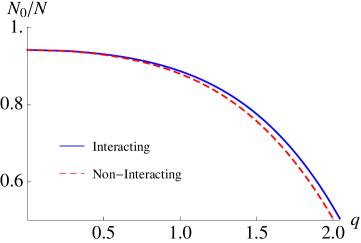
Figure 5: (Color online) In this plot, we show the condensate fraction $N_{0}/N$ for both interacting and non-interacting gases, as a function of the lattice depth $q=V_{0}/4E_{\rm r}$ at temperature $T=0.1E_{\rm r}$. The condensate fraction decreases with increasing lattice depth $q$, approaching the phase transition. We also observe that the condensation fraction for the interacting gas is larger than that of the non-interacting gas. Here the system is at unit filling, with system parameters consistent with those of Ref. natphys:trotzky .

Within our theory, interaction effects become stronger below ${T_{\rm c}}$ in the superfluid phase, as the condensate becomes occupied. However, for system parameters consistent with Ref. natphys:trotzky , we still find interaction effects to be small. This is illustrated in Fig. 5, which shows our theoretical prediction for the condensate fraction, $N_{0}/N$ vs. normalized optical lattice depth, $q=V_{0}/4E_{\rm r}$ for the case of $T=0.1E_{\rm r}$, along with the case of vanishing interactions for comparison. We see that interaction effects are small for any $q$, but are smallest for $q\to 0$ (the case of no optical lattice) with the interacting condensate fraction being slightly larger than the non-interacting case at larger $q$.

Within our scheme, we do not expect to be able to capture the suppression of ${T_{\rm c}}$ towards the Mott phase and, as we have seen, we also find negligible effects of interactions away from the deep Mott insulator regime for system parameters consistent with the Trotzky et al. results. Next, we turn to the case of larger filling and larger interaction strength, where interaction effects may be more significant.

IV.2 Interaction effects at large filling

Figure 6: (Color online) In this plot, we show the trend of the transition temperature ${T_{\rm c}}$ with varying lattice depth $q=V_{0}/4E_{\rm r}$ for the case of filling $f=5$ and other system parameters consistent with Ref. natphys:trotzky .

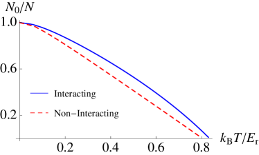
Figure 7: (Color online) Plot of the condensate fraction for both non-interacting and interacting gases, as a function of temperature, over the temperature range from $T=0$ to ${T_{\rm c}}$ (where the fraction becomes zero), with filling $f=5$ and normalized optical lattice depth $q=1.75$, and other system parameters consistent with Ref. natphys:trotzky .

Within our Hartree-Fock approach interaction effects arise because the boson density acts as an effective spatially-varying single-particle potential. At larger filling, the boson density is higher and one may expect interaction effects to be stronger. In the present section we illustrate this by increasing the system filling to $f=5$ while keeping all other parameters consistent with Ref. natphys:trotzky .

Figure 6 shows the transition temperature as a function of normalized optical lattice depth for this case, showing a slight separation between the curves with increasing $q$. Although ${T_{\rm c}}$ is only slightly enhanced by interactions, Fig. 7, which plots the condensate fraction below ${T_{\rm c}}$ for the case of $q=1.75$, shows a clear enhancement of the condensate fraction (solid curve) relative to the non-interacting case (dashed curve). We interpret this, physically, as being due to the fact that, as more bosons enter the condensate below ${T_{\rm c}}$, the spatially-inhomogeneous nature of the wave function leads, self-consistently, to a larger effect of interactions on system properties. At the lowest temperatures, however, all bosons enter the condensate, so that both curves must eventually merge at $N_{0}/N=1$ for $T\to 0$, as seen in Fig. 7.

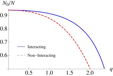
Figure 8: (Color online) In this plot, we show the condensate fraction $N_{0}/N$ for both interacting and non-interacting gases, as a function of the lattice depth $q=V_{0}/4E_{\rm r}$ at temperature $T=0.1E_{\rm r}$. Here the system is at unit filling, with system parameters consistent with those of Ref. natphys:trotzky , except with a large scattering length $a_{s}=0.1a$.

IV.3 Interaction effects at large scattering length

Next, we investigate the effect of increasing the $s$-wave scattering length. To characterize the interactions, we note that, relative to the lattice spacing, the Trotzky experiments are at $a_{s}/a\simeq 1.3\times 10^{-2}$, which we can regard as being at weak coupling. However, larger scattering lengths are indeed achievable for cold atoms in optical lattices, as shown, for example, by the experiments of Mark et al. prl:marknageri on cesium BEC’s. To explore this, we studied bosons in optical lattices within our self-consistent approach, using the same parameters as the Trotzky et al. experiments natphys:trotzky but with a larger scattering length $a_{s}\simeq 0.1a$. As shown in Fig. 8, this leads to a rather large shift of the condensate fraction, relative to the non-interacting case, that grows with increasing optical lattice depth.

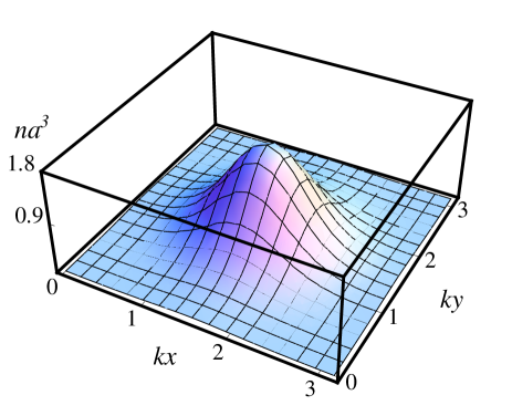
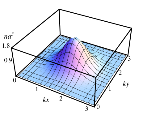
Figure 9: (Color online) The top panel shows the local density in a unit cell for $kz=\pi/2$ in the presence of repulsive interactions. Here, system parameter are the same as those of Ref. natphys:trotzky but with a larger scattering length $a_{s}\simeq 0.1a$ and filling $f=2.83$. For comparison, the bottom panel shows the non-interacting case.

IV.4 Interaction effects on local boson density

We have argued that the enhancement of the condensate fraction at a particular temperature and optical lattice depth, relative to the non-interacting case, occurs because the local boson density is more spatially uniform in the presence of repulsive interactions, enhancing superfluidity. Computing the local density in a unit cell requires solving for our self consistent parameters $c$ and $\bar{q}$, along with the system chemical potential $\mu$ and then inputing these values into the local density Eq. (35), requiring a sum over the Mathieu function indices $\mbox{\boldmath$\nu$}=(\nu_{x},\nu_{y},\nu_{z})$. After carrying out this numerically-intensive procedure, we find that the local density in a unit cell indeed becomes broadened within a unit cell with increasing repulsive interactions, as shown in Fig. 9 for $kz=\pi/2$. Here the top panel is the interacting case, and the bottom panel is the non-interacting case, with the system temperature given by $k_{\rm B}T/E_{\rm r}=0.3846$, filling $f=2.83$, optical lattice depth $q=2$, and $a_{s}=0.1a$. For these parameters, the non-interacting plot is at ${T_{\rm c}}$ while the interacting plot is slightly below ${T_{\rm c}}$.

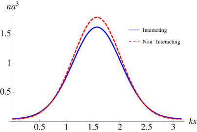
Figure 10: (Color online) This plot shows the interacting boson density (solid curve) as a function of the spatial variable $x$ in a unit cell at $ky=\pi/2$, $kz=\pi/2$ (crossing the unit cell center), showing a suppression of the central boson density relative to the non-interacting case (dashed curve).

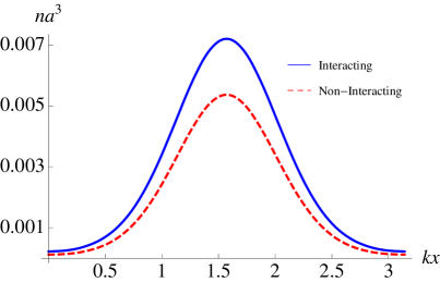
Figure 11: (Color online) This plot shows the interacting boson density (solid curve) as a function of the spatial variable $x$ in a unit cell at $ky=\pi/8$, $kz=\pi/8$ (near the unit cell edge), showing an increase of the central boson density relative to the non-interacting case (dashed curve).

For a more quantitative comparison, in Figs. 10 and 11 we show the local density vs. position for at the center $ky=\pi/2$, $kz=\pi/2$ (Fig. 10) and near the edge $ky=\pi/8$, $kz=\pi/8$ (Fig. 11), showing that the boson density is more homogeneous in the interacting case, with the interacting density smaller near the unit cell center and larger at the edge of the unit cell, relative to the non-interacting case.

IV.5 Boson momentum distribution

In ultracold atom experiments, a BEC is indicated by peaks (i.e. maxima) in the images of the cloud after free expansion that reflect the boson momentum distribution in the initially trapped cloud. In this section, we calculate the momentum distribution to see how interaction changes the superfluid state. As reviewed in Appendix B, the real space boson density after free expansion probes the momentum distribution:

$$n(\mathbf{k})=N_{0}|\Phi_{0}(\mathbf{k})|^{2}+\sum_{i\neq 0}|\Phi_{i}(\mathbf{k})|^{2}n_{\rm B}(\epsilon_{i}-\mu),$$ (41)

where $\Phi(\mathbf{k})$ is the Fourier transformed Mathieu wave function. By inserting the wave functions and energy levels obtained from our self-consistent scheme into Eq. (41), we are able to obtain the boson momentum distribution. Note that we are not considering interaction during the expansion.

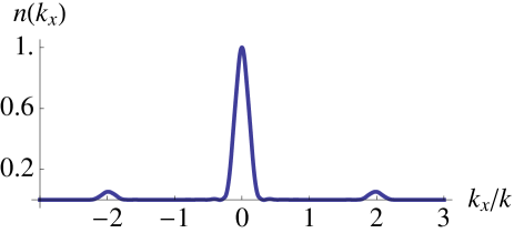
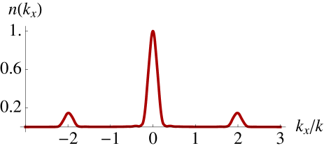
Figure 12: (Color online) The boson momentum distribution as a function of $k_{x}$ for $k_{y}=0$ and $k_{z}=0$, with system parameters given in the main text. Both plots are normalized so that $n(0)=1$. The top panel shows the interacting case, and the bottom panel shows the non-interacting case, with the height of the side peaks being smaller in the interacting case reflecting a more spatially-uniform Bose gas.

Most cold atom experiments with optical lattices involve a background smoothly-varying parabolic trap. In our analysis, we did not account for this, but instead studied a “box”-shaped trap possessing a periodic optical lattice potential along with hard-wall boundary conditions to take into account the finite-size initial cloud. We considered a cubic system with length $L=\pi N_{\rm s}/k$ with $N_{\rm s}=10$ lattice sites along each direction (containing $N_{\rm sites}=10^{3}$ total sites). We note here that such box-shaped traps have recently been achieved experimentally prl:gaunt .

In Fig. 12, we show our results for the boson momentum distribution Eq. (41) at $k_{y}=k_{x}=0$, with the same system parameters as in the preceding section, with the top panel being the interacting case, and the bottom panel being the non-interacting case. Each plot is normalized so that $n({\bf k})=1$ at ${\bf k}=0$. The side-peaks are expected for a BEC in a periodic optical lattice (as observed by Greiner et al. nat:greiner ), and should occur for ${\bf k}$ equal to any reciprocal lattice vector. The side-peaks in Fig. 12 occur at $k_{x}=\pm\frac{2\pi}{a}=\pm\frac{2}{k}$. The height of the side peaks, relative to the central peak, reflects the degree of spatial inhomogeneity of the BEC, as can be seen by noting the limiting case of a spatially-uniform BEC, which will have only a central peak at ${\bf k}=0$. Thus, since the side-peaks are smaller in the interacting case, we argue that the boson momentum distribution also reflects the spatial homogenization of the cloud in the presence of repulsive interactions.

V Conclusion

In this paper, we studied the effect of short range repulsive interactions on the properties of bosons in periodic optical lattices. For a uniform boson gas, the effect of such interactions on the superfluid transition temperature ${T_{\rm c}}$ has been argued for decades, with both positive and negative ${T_{\rm c}}$ shifts having been reported rmp:andersen . The consensus is that ${T_{\rm c}}$ increases linearly with scattering length $a_{s}$ Baym99 .

In contrast, bosons in a deep optical lattice, characterized by the Bose Hubbard model (BHM), exhibit a suppression of ${T_{\rm c}}$ with increasing repulsive interactions. Given that a system consisting of bosons in a periodic optical lattice with lattice depth $V_{0}$ continuously interpolates between the limiting cases of a uniform gas (for $V_{0}\to 0$) and the BHM (for $V_{0}\gg E_{r}$), then one may expect an increase of ${T_{\rm c}}$ with $a_{s}$ away from the BHM regime.

Instead of the commonly used tight-binding approach that leads to the BHM, our theoretical study of this system started from the exact single-particle states of bosons in an optical lattice, satisfying the Mathieu equation, an approach that can be particularly useful at large boson filling or when many single-particle bands are occupied. Interaction effects were accounted for using a self-consistent Hartree-Fock approximation, in which the spatially-inhomogeneous boson density leads to an effective reduction of the optical lattice depth.

We applied this scheme to quantify the effects of inter-atomic interactions on the properties of bosons in an optical lattice, as exhibited in the comparison between observables of non-interacting and interacting systems. We found that interactions increase the superfluid transition temperature and the condensate fraction, and also homogenizes the local boson density (as would be seen in the local density and also the momentum distribution as probed in time-of-flight experiments).

An obvious weakness of our approach is that we are unable to capture the Mott insulating regime for bosons in optical lattices occurring for integer filling at large optical lattice depth. A natural extension of our work will be to understand the emergence of the Mott insulating phase within the Mathieu equation approach (i.e., without making the BHM approximation which provides a natural picture of the Mott insulating state). Such an extension would lead to a more complete understanding of the properties of interacting BEC’s in optical lattices.

This work was supported by National Science Foundation Grant No. DMR-1151717. This work was supported in part by the National Science Foundation under Grant No. PHYS-1066293 and the hospitality of the Aspen Center for Physics. DES acknowledges support from the German Academic Exchange Service (DAAD) and the hospitality of the Institute for Theoretical Condensed Matter physics at the Karlsruhe Institute of Technology.

Appendix A Hartree-Fock Approximation

We use Hartree-Fock Approximation to describe the inter-atomic interaction. Hartree-Fock approximation assumes a dependence of the system’s self energy on the atomic density.

Consider a translationally invariant system or a system possessing discrete translational invariance (such as in a periodic potential). The Dyson’s Equation is

$$G(\mathbf{r},\mathbf{r}^{\prime};\tau,\tau^{\prime})=G_{0}(\mathbf{r},\mathbf{r}^{\prime};\tau,\tau^{\prime})+\int d^{3}r_{1}d^{3}r_{2}d\tau_{1}d\tau_{2}~{}G_{0}(\mathbf{r},{\mathbf{r}_{1}}^{\prime};\tau,\tau_{1})\Sigma(\mathbf{r}_{1},\mathbf{r}_{2};\tau_{1},\tau_{2})G(\mathbf{r}_{2},\mathbf{r}^{\prime};\tau_{2},\tau^{\prime}),$$ (42)

where $G$ and $G_{0}$ are the Green’s functions of spatial coordinates ${\bf r}$, ${\bf r}^{\prime}$ and imaginary time $\tau$, $\tau^{\prime}$ respectively for the entire system and for the bare system, and $\Sigma$ is the self energy characterizing the contribution from interaction. On the other hand, we have

$$G({\bf r},{\bf r}^{\prime},\tau,\tau^{\prime})=-\left<T_{\tau}\Psi({\bf r},\tau)\Psi^{\dagger}({\bf r}^{\prime},\tau^{\prime})e^{-\int_{0}^{\beta}d\tau H_{1}(\tau)}\right>,$$ (43)

where $H_{1}$ is given by Eq. (2). To derive the Hartree-Fock term, we expand to the first order (denoting $x=({\bf r},\tau)$, and similarly for $x^{\prime}$ and $x_{1}$),

$$\begin{split}&G(x,x^{\prime})=\\ &-\left<T_{\tau}\Psi(x)\Psi^{\dagger}(x^{\prime})\Big{[}1-\frac{g}{2}\int dx_{1}~{}\Psi^{\dagger}(x_{1})\Psi^{\dagger}(x_{1})\Psi(x_{1})\Psi(x_{1})\Big{]}\right>,\end{split}$$ (44)

where the coupling constant $g=4\pi\hbar^{2}a_{s}/m$. In the above Green’s function, there are two ways for $\Psi(x)$ to contract with the two $\Psi^{\dagger}(x_{1})$ factors, and there are two ways for $\Psi^{\dagger}(x^{\prime})$ to contract with the two $\Psi(x_{1})$ factors. Therefore, with $G_{0}(x,x^{\prime})=-\left<T_{\tau}\Psi(x)\Psi^{\dagger}(x^{\prime})\right>$, we have

$$G(x,x^{\prime})=G_{0}(x,x^{\prime})-2g\int dx_{1}~{}G_{0}(x,x_{1})G_{0}(x_{1},x_{1})G_{0}(x_{1},x^{\prime}).$$ (45)

Comparing Eq. (45) with Eq. (42), we obtain

$$\Sigma(x_{1},x_{2})=-2gG_{0}(x_{1},x_{1})\delta(x_{1}-x_{2}).$$ (46)

Since $G_{0}(x_{1},x^{+}_{1})=-n(x_{1})$, the boson density, we come to

$$\Sigma(x,x^{\prime})=2gn(x)\delta(x-x^{\prime}),$$ (47)

namely, the Hartree-Fock Approximation.

Appendix B Free Expansion

The superfluid state of bosons is usually shown in experiments by absorption imaging of the freely expanded cloud read . In this process, the trapping potential is abruptly turned off, the atomic gas undergoes a period of time-of-flight free expansion. The absorption image provides information about the density profile, which is related to the initial momentum distribution. Atoms that are initially of the same state will gather together in the real space, therefore density peaks in the image indicate Bose-Einstein condensate.

Assume the trapping potential is turned off at $t=0$. The time dependent density

$$n(\mathbf{r},t)=\mathrm{Tr}\rho_{\mathcal{H}}(t)\hat{n}(\mathbf{r})=\mathrm{Tr}\rho_{\mathcal{H}}(t)\hat{\Phi}^{\dagger}(\mathbf{r})\hat{\Phi}(\mathbf{r}),$$ (48)

where $\hat{\Phi}(\mathbf{r})$ and $\hat{\Phi}^{\dagger}(\mathbf{r})$ are field operators, $\rho_{\mathcal{H}}$ is the density matrix for the time dependent Hamiltonian which is written as

$$\mathcal{H}(t)=H_{0}+\Theta(-t)H_{\rm trap},$$ (49)

where

$$\Theta(t)=\left\{\begin{array}[]{l}0,~{}~{}(t\leq 0);\\ 1,~{}~{}(t>0).\end{array}\right.$$ (50)

The Hamiltonian is entirely time invariant before $t=0$, we can denote $\mathcal{H}(t<0)\equiv\mathcal{H}_{\infty}$. The density after the trap potential is turned off is obtained by

$$n(\mathbf{r},t>0)=\mathrm{Tr}\rho_{\mathcal{H}_{\infty}}\hat{n}(\mathbf{r},t),$$ (51)

where $\hat{n}(\mathbf{r},t)\equiv e^{itH_{0}}{n}(\mathbf{r})e^{-itH_{0}}$. $\rho_{\mathcal{H}_{\infty}}\equiv\rho_{\mathcal{H}}(t<0)$ is the initial density matrix at $t=0$. The field operators $\hat{\Phi}(\mathbf{r})$ can be expanded either in the eigenstates of $H_{0}$ or in the eigenstates of $\mathcal{H}_{\infty}$, and the former of which are just plane waves. Therefore we can obtain the density matrix $\rho_{\mathcal{H}_{\infty}}$ by equating the two expansions, and plug into Eq. (51) to solve for the density $n(\mathbf{r},t>0)$. The result is

$$n(\mathbf{r},t)=\sum_{i}\sum_{\mathbf{k}}\mid e^{itE_{\mathbf{k}}-i\mathbf{k}\cdot\mathbf{r}}\tilde{\phi}_{i}(\mathbf{k})\mid^{2}n_{\rm B}(\varepsilon_{i}-\mu),$$ (52)

where $\tilde{\phi}_{i}(\mathbf{k})$ is the Fourier transform of the eigenfunction of $\mathcal{H}_{\infty}$. If we translationally move in the momentum space from $\mathbf{k}$ to $\mathbf{k}+\frac{m\mathbf{r}}{t}$, where $\mathbf{k}\ll\frac{m\mathbf{r}}{t}$, Eq. (52) becomes

$$n(\mathbf{r},t)\propto\sum_{i}\left|\tilde{\phi}_{i}(\mathbf{r}m/t)\right|^{2}n_{\rm B}(\varepsilon_{i}-\mu).$$ (53)

We note that, up to an overall prefactor, the right side of Eq. (53) is the momentum distribution $n(\mathbf{k})$ of the initial trapped gas, measured at momentum $\mathbf{k}=m\mathbf{r}/t$. Thus, the density profile of the expanded cloud allows experimentalists to probe the momentum distribution of the trapped cloud.

References

- (1) I. Bloch, J. Dalibard, and W. Zwerger, Rev. Mod. Phys. 80, 885 (2008).
- (2) M. Lewenstein, A. Sanpera, V. Ahufinger, B. Damski, A. Sen(De) and U. Sen, Adv. Phys. 56, 243 (2007).
- (3) D. Jaksch, C. Bruder, J. I. Cirac, C. W. Gardiner, and P. Zoller, Phys. Rev. Lett. 81, 3108 (1998).
- (4) M. P. A. Fisher, P. B. Weichman, G. Grinstein, and D. S. Fisher, Phys. Rev. B 40, 546 (1989).
- (5) M. Greiner, O. Mandel, T. Esslinger, T. W. Hänsch, and I. Bloch, Nature 415, 39 (2002).
- (6) M. Köhl, H. Moritz, T. Stöferle, C. Schori, and T. Esslinger, J. Low Temp. Phys. 138, 635 (2005).
- (7) I. B. Spielman, W. D. Phillips, and J. V. Porto, Phys. Rev. Lett. 98, 080404 (2007).
- (8) J. Mun, P. Medley, G. K. Campbell, L. G. Marcassa, D. E. Pritchard, and W. Ketterle, Phys. Rev. Lett. 99, 150604 (2007).
- (9) N. Gemelke, X. Zhang, C.-L. Hung, and C. Chin, Nature 460, 995 (2009).
- (10) S. Trotzky, L. Pollet, F. Gerbier, U. Schnorrberger, I. Bloch, N. V. Prokof’ev, B. Svistunov, and M. Troyer, Nature Physics 6, 998 (2010).
- (11) C. Becker, P. Soltan-Panahi, J. Kronjäger, S. Dörscher, K Bongs, and K Sengstock, New J. Phys. 12, 065025 (2010).
- (12) M. Endres, M. Cheneau, T. Fukuhara, C. Weitenberg, P. Schauß, C. Gross, L. Mazza, M. C. Bañuls, L. Pollet, I. Bloch, and S. Kuhr, Science 334, 200 (2011).
- (13) M. J. Mark, E. Haller, K. Lauber, J. G. Danzl, A. J. Daley, and H.-C. Nägerl, Phys. Rev. Lett. 107, 175301 (2011).
- (14) X. Zhang, C.-L. Hung, S.-K. Tung, and C. Chin, Science 335, 1070 (2012).
- (15) B. Capogrosso-Sansone, N.V. Prokof’ev, and B.V. Svistunov, Phys. Rev. B 75, 134302 (2007),
- (16) Handbook of Mathematical Functions, edited by M. Abramowitz and I. A. Stegun (Dover, New York, 1972).
- (17) W. Zwerger, J. Opt. B: Quantum and Semiclassical Optics 5, S9 (2003).
- (18) D. McKay, M. White, and B. DeMarco, Phys. Rev. A 79, 063605 (2009).
- (19) G. Baym, J.-P. Blaizot, M. Holzmann, F. Laloë, and D. Vautherin, Phys. Rev. Lett. 83, 1703 (1999).
- (20) J. O. Andersen, Rev. Mod. Phys. 76, 599 (2004).
- (21) NIST Digital Library of Mathematical Functions, http://dlmf.nist.gov/ .
- (22) A.L. Gaunt, T. F. Schmidutz, I. Gotlibovych, R. P. Smith, and Z. Hadzibabic, Phys. Rev. Lett. 110, 200406 (2013).
- (23) N. Read and N.R. Cooper, Phys. Rev. A 68, 035601 (2003).