The Dune-ALUGrid Module

Abstract

In this paper we present the new Dune-ALUGrid module. This module contains a major overhaul of the sources from the ALUGrid library and the binding to the Dune software framework. The main improvements concern the parallel feature set of the library. The main changes include user-defined load balancing, parallel grid construction, and an redesign of the 2d grid which can now also be used for parallel computations. In addition many improvements have been introduced into the code to increase the parallel efficiency and to decrease the memory footprint.

The original ALUGrid library is widely used within the Dune community due to its good parallel performance for problems requiring local adaptivity and dynamic load balancing. Therefore, this new model will benefit a number of Dune users. In addition we have added features to increase the range of problems for which the grid manager can be used, for example, introducing a 3d tetrahedral grid using a parallel newest vertex bisection algorithm for conforming grid refinement. In this paper we will discuss the new features, extensions to the Dune interface, and explain for various examples how the code is used in parallel environments.

Keywords: Numerical software, Adaptive-parallel grid, Load Balancing, Dune

1 Introduction

The origin of the ALUGrid package dates back to the late 20th century as part of the PhD thesis of Bernhard Schupp [32]. Back then, the task was to develop a software that could solve the compressible Euler equations of gas dynamics with a Finite Volume scheme on a parallel computer in 3d including local grid adaptivity. To achieve this task Schupp implemented a 3d hexahedral adaptive mesh including dynamic load balancing based on METIS graph partitioning [19]. Later, support for tetrahedral elements was added to the grid manager and the code was successfully used to simulate solar eruption phenomena based on the MHD equations [13]. Shortly after this, the library was used to implement the Dune grid interface [10]. The ALUGrid bindings were the first grid implementation providing the full interface for an adaptive, distributed grid including dynamic load balancing. It has been shown that ALUGrid is a very efficient implementation of the Dune grid interface. For an explicit Finite Volume scheme, the performance loss introduced by the Dune bindings is roughly $10\%$ compared to the native ALUGrid implementation [5, 10, 21]. At that time also a serial 2d simplex grid was added to the code basis. The following releases of the software saw only maintenance work with no substantial increase in the feature set.

In this paper the first major overhaul of the ALUGrid code basis is described. Originally, ALUGrid was available as a stand alone library with a quite complex user API. Consequently, ALUGrid was used exclusively through the bindings available in the Dune-Grid module. To reduce maintenance and improve usability we integrated both, the original ALUGrid library and its bindings to Dune, into the new Dune-ALUGrid module. In addition a number of new features have been added and the efficiency of the code has been increased while the memory footprint has been substantially reduced.

ALUGrid is a capable and reliable parallel-adaptive grid manager and has been used in codes based on Dune, for example, in life science applications [2, 7], in the simulation of nanotechnology [27, 15], in simulations related to numerical weather and climate prediction [9, 28], simulation of reactive flow in a moving domain [24], or in subsurface simulations [14] and other works.

Within Dune the other unstructured grid manager capable of parallel-adaptive computations is UG [25] with the UGGrid realization of the Dune grid interface. A comparison for time-explicit applications with and without adaptivity using the different grid implementations available in Dune is presented in [23].

Besides a vast number of structured or Cartesian grid managers supporting adaptive refinement (see http://math.boisestate.edu/~calhoun/www_personal/research/amr_software/) there exist a few other open source unstructured grid managers (at present without bindings to Dune), for example, deal.II [4] which is build on top of p4est [11]. Hexahedral grids with non-conforming refinement are provided. Excellent scalability has been reported. As a drawback, the macro mesh has be present on every core limiting the macro mesh size. Other very capable unstructured grid managers are, for example, the ”Flexible Distributed Mesh Database (FMDB)” [36], libMesh [20], or AMDIS [34]. The latter is providing tetrahedral elements with bisection refinement.

In this paper we present work done in recent years to improve the useablility, efficiency, and reduce maintanace cost of ALUGrid:

In the previous versions of ALUGrid the implementation of the 2d and 3d grids were completely seperate. This resulted in a disjoint set of features with the 2d grid implementing bisection not available for the 3d grid while at the same time the 2d grid did not provide any parallel features. In Dune-ALUGrid the original code for the 2d grid has been removed. Grids in two space dimensions or surface grids are now implemented by embedding them into three space dimensions, making it possible to directly use the 3d grid implementation. The main advantage of this is the significant reduction in code maintance while at the same time all improvements in performance or feature set of the 3d code will be directly available also for 2d grids. Furthermore, since conforming bisection is now also available in 3d, this merge has not resulted in any loss of functionality.

To simplify the installation, the Dune bindings and the library itself have been combined in a single Dune module. This module includes a number of new features, which make the ALUGrid implementation a lot more flexible and make it possible to use it through Dune for a wider range of problems:

• extension to implement a wider range of methods:
  the main extension is conforming grid refinement implemented in the parallel 3d code. Furthermore the 2d grid can be used for distributed computations so that the 2d and 3d code now share the same feature set. In addition the support for quadrilateral and surface grids in 2d and periodic boundary treatment in 3d for parallel computations has been improved.

• increasing usability and efficiency:
  the memory footprint is considerably reduced (Section 2.1), a cleaner interface for callback adaptation, which was partially available before, is discussed in Section 3.6.

• increasing usability and efficiency for parallel computation:
  new features include: parallel grid construction (discussed in Section 3.3), backup and restore (discussed in Section 3.4), overlapping communication and computation, (discussed in Section 3.5), wider range of load balancing algorithms (including internal implementations), and user-defined partitioning algorithms (these are discussed in Sections 3.7 and 3.8). In summary Dune-ALUGrid now provides

  • intrinsic partitioning based on space filling curves, making Dune-ALUGrid independent of other packages,

  • bindings for the library Zoltan [8],

  • an interface for user-defined partitioning.

In Section 2 we describe how we have evaluated the performance of the Dune-ALUGrid module and report on a number of different strong and weak scaling results obtained on both a computing cluster and a highly integrated high performance computing system. Following, in Section 3, we present the new features and interface extensions from a user’s point of view, Finally we make some concluding remarks and discuss some open issues with this module.

For a successful and satisfactory reading of this paper it is recommended to be familiar with the Dune papers [5, 6] and the terminology used therein.

2 Performance Testing

The aim of [32] was to develop an efficient parallel implementation of an adaptive explicit Finite Volume scheme. These schemes are widely used for solving hyperbolic conservation laws. The appearance of steep gradients or shocks in the solution make grid adaptivity a good choice to increase the efficiency of a scheme. These shocks move in time requiring the refinement zones to move with the shocks and coarsening to take place behind them. In combination with a domain decomposition approach for parallel computation, this means that the load is difficult to balance between processors and dynamic load balancing is essential. So in each time step the grid needs to be locally refined or coarsened and the grid has to be repartitioned quite often. What makes this problem extremely challenging is the fact that evolving the solution from one time step to the next is very cheap since the update is explicit and no expensive linear systems have to be solved. So adaptivity and load balancing will dominate the computational cost of the solver. Both of these steps require global communication steps and the communication of possibly a significant amount of data and are therefore difficult to implement even with a moderate amount of parallel efficiency (see for example [11]).

Since this is a very demanding problem for a parallel code, we have decided to continue using explicit Finite Volume schemes to measure the performance of the Dune-ALUGrid module. Grid performance plays a role in matrix-free methods where frequent grid iteration occurs in order to evaluate differential operators even if the used discrete function space is of higher order. In contrast, the performance of implicit matrix-based methods will have a stronger dependency on the efficiency of the parallel solver package than on the grid implementation. Therefore, testing implicit methods would not provide as much insight into the performance of the grid module itself.

As a simple example, we consider the scalar transport equation

$$\partial_{t}u+\nabla\cdot\bigl{(}(1.25,1.25,0)^{T}\,u\bigr{)}=0$$

with suitable initial and boundary data (see examples/problem-transport.hh ). In the adaptive Finite Volume scheme we use an upwind numerical flux and a jump indicator to trigger grid adaptation.

For a more damanding example, we also apply this scheme to the Euler equations of gas dynamics

$$\partial_{t}\begin{pmatrix}\rho\\ \rho\,\vec{v}\\ \epsilon\end{pmatrix}+\nabla\cdot\begin{pmatrix}\rho\,\vec{v}\\ \rho\,\vec{v}\otimes\vec{v}+p\,\mathbb{I}\\ (\epsilon+p)\,\vec{v}\end{pmatrix}=0,$$

where $\mathbb{I}\in\mathbb{R}^{d\times d}$ denotes the identity matrix. We consider an ideal gas, i.e., $p=(\gamma-1)\,(\epsilon-\frac{1}{2}\,\rho\,\lvert\vec{v}\rvert^{2})$, with the adiabatic constant $\gamma=1.4$. In the adaptive scheme, we use an HLLC numerical flux [33] in the evolution step and the relative jump in the density to drive the grid adaptation. Two typical test problems found in the literature, the Forward Facing Step and the interaction between a shock and a bubble (see [12] and references therein) are implemented (see examples/problem-euler.hh ).

To benchmark solely adaptation and load balancing, we implemented a third, even more demanding test case. Instead of using the solution to a partial differential equation to determine the zones for grid refinement and coarsening, a simple boolean function $E\mapsto\eta_{E}$ is used (see examples/problem-ball.hh ). We refine all elements located near the surface of a ball rotating around the center of the 3d unit cube:

$$\boldsymbol{y}(t) :=\Bigl{(}\tfrac{1}{2}+\tfrac{1}{3}\cos(2\pi t),\tfrac{1}{2}+\tfrac{1}{3}\sin(2\pi t),\tfrac{1}{2}\Bigr{)}^{T},$$ (1)

$$\eta_{E} :=\begin{cases}1&\text{if }0.15<|\boldsymbol{x}_{E}-\boldsymbol{y}(t)|<0.25,\\ 0&\text{otherwise,}\end{cases}$$

where $\boldsymbol{x}_{E}$ denotes the barycenter of the element $E$. A cell $E$ is marked for refinement, if $\eta_{E}=1$ and for coarsening otherwise. This sort of problem was also studied in [32]. Since the center of the ball is rotating, frequent refinement and coarsening occurs, making this an excellent test for the implemented adaptation and load balancing strategies.

2.1 Memory Consumption

Memory consumption has become more and more critical for any numerical software since the overall memory available per core has declined lately. First we need to give a short summary of the data structure used to store grid elements: A vertex stores its coordinates, an edge stores pointers to the two vertices, a quadrilateral face stores pointers to the four edges and a hexahedron stores pointers to the six faces it consists of. For example, the memory consumption of a vertex on a 64bit architecture is $56$ bytes due to the storage of coordinates ($3$ double result in $24$ bytes), $8$ bytes for the vtable (all interfaces in ALUGrid use dynamic polymorphism), $8$ bytes for a pointer to the grid class, and another $12$ bytes for flags, reference counting, and index storage, which due to padding this adds up to $56$ bytes.

Table 1: Memory consumption by ALUGrid’s entities in bytes (in braces we put the memory consumption in ALUGrid’s 1.52 version).

type	tetra	hexa	macro tetra	macro hexa
vertex	56 5(64)	56 5(64)	80 5(80)	80 5(80)
edge	56 (136)	56 (136)	64 (144)	64 (144)
face	88 (160)	96 (174)	96 (168)	104 (184)
element	96 (160)	112 (184)	104 (168)	120 (192)

Depending on the size of the macro grid and the face/edge to element ratio a hexahedral grid consumes between $700$ and $800$ bytes per element. The tetrahedral version of the grid consumes between $350$ and $400$ bytes per element. Note that these numbers strongly depend on the macro grid chosen and might vary for other macro grids. For the old version $1.52$ storing a hexahedral element needed between $1\,300$ and $1\,500$ bytes. For a tetrahedral element version $1.52$ needed between $650$ and $750$ bytes. In Figure 1 we show the memory consumption for the old and the new version for the ball test case with adaptation using the refinement from (1). In summary the memory consumption has been reduced by about a factor of $2$.

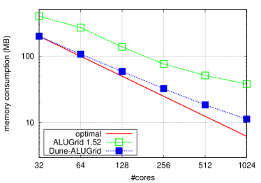
(a) cube

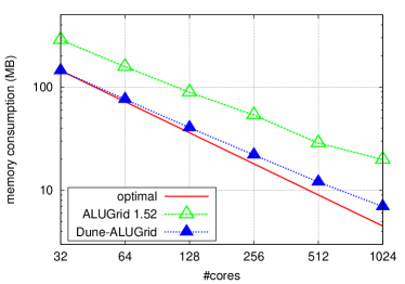
(b) simplex

Figure 1: Comparison of memory usage for the old and the new version. Both version use dlmalloc as memory allocator. The $1.52$ version has been patched for this purpose.

In an adaptive grid, entities are frequently created during refinement and destroyed during coarsening. As ALUGrid allocates memory for each grid entity separately, efficient memory allocation and deallocation plays an important part in this process. To allow for customization, ALUGrid derives all entities from an object called MyAlloc , which contains overloaded operators new and delete . Two such objects are shipped with Dune-ALUGrid.

default

does not overload the operators new and delete , so that standard C++ memory allocation is used. This is the default memory allocation used.

dlmalloc

makes use of Doug Lea’s memory allocator ( dlmalloc ) [26], which can be downloaded from http://g.oswego.edu/dl/html/malloc.html. If the configure option
--with-dlmalloc=PATH is provided specifying a path to the dlmalloc installation, dlmalloc will be used for allocation of grid entities.

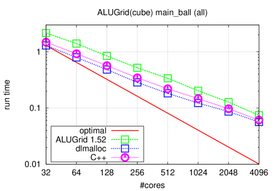
Figure 2: Comparison of run times for the different memory allocation strategies. The memory allocation using Doug Lea’s memory allocator [26] performed best, the strategy used in ALUGrid 1.52 performed worst and has therefore been removed in the new version. For load balancing we used the internal space filling curve approach with locally computed linkage (partition method id 4).

In Figure 2 we present a comparison of runtimes between the different memory allocation strategies. The former internal ALUGrid implementation based on std::map and std::stack has been removed since it did not lead to performance gains, anymore. For adaptation with the ball refinement from equation (1) using dlmalloc around $10\,\%$ less CPU time is consumed in comparison to the standard C++ memory allocation on Yellowstone [1].

As mentioned in the introduction the codes for the 2d and 3d grid have been unified. The only drawback of embedding the 2d into a 3d grid is an increase in the memory requirements of the 2d grid. For example a 2d quadrilateral grid is modelled using a 3d hexahedral grid by replacing each quadrilateral by one hexahedron. Effectively this leads to a doubling of the memory usage in this case. For a triangular grid the resulting increase in memory usage is less severe. This is confirmed by the results shown in Figure 3a. This increase in memory consumption in the new version in compensated by improvements in performance, as can be seen in Figure 3b.

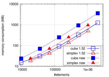
(a) memory

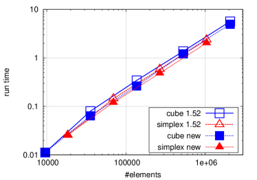
(b) run times

Figure 3: Comparison of memory usage and run times for the 2d version in the old and the new implementation. Both versions use dlmalloc as memory allocator. The $1.52$ version has been patched for this purpose.

2.2 Scaling results

We start with testing the new parallel version of the 2d code. In Figure 4 we present the results of a 2d version of the shock-bubble interaction problem taken from [12] using a small size computer cluster consisting of 20 Intel Core-i3 2100 (Sandy-Bridge) desktop computers connected via standard gigabit ethernet. The curves represent different parts of the code (solve: computation and synchronization of the update vector, comm: global synchronization of time step, adapt: grid adaptation, and lb: load balancing). Finally we show the total runtime. Note that there are some small parts of the time loop not seperately shown so that the total runtime is not exactly the sum of the four parts shown. For the dynamic load balancing we use the space filling curve approach newly implemented in Dune-ALUGrid, see Section 3.7. The grid load balancing is checked every $25^{th}$ time step and is performed when the number of elements between the largest and smallest partition differs by $20\%$ or more.

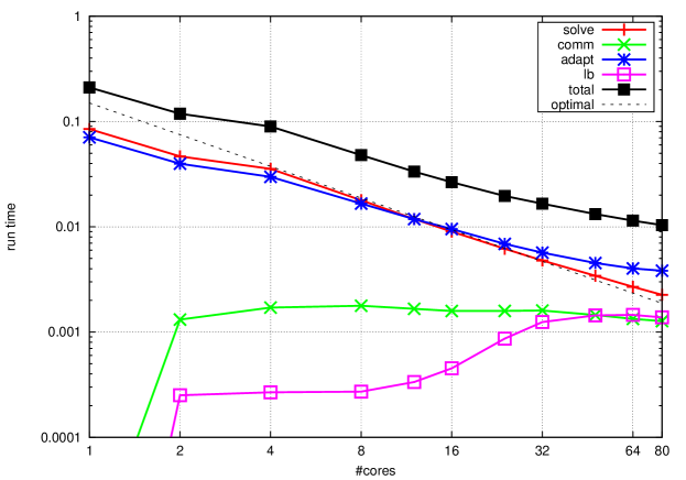
Figure 4: Strong scaling results for 2d Euler shock-interaction problem on a small size computer cluster.

As we can see the Finite Volume part of the code scales very well up to $64$ cores. The overall scaling is still acceptable. Note that we are using hyperthreading to execute four processes per node although these are dualcore machines. Parallel efficiency increases by about $10\%$ when only two proceses are put on one node but the runtime using a given number of nodes is quite a bit higher. Note that the number of degrees of freedom was quite small in this simulation so that even on a few cores, the cost for the solve step and for the adaptation are comparable. Thus the total runtime more or less follows the curve for the adaptation cost leading to $50\%$ efficiency going from $4$ to $64$ cores while the solve step itself is still close to optimal.

We repeated the same test but now using the 3d grid (Figure 5). The macro grid was larger in this simulation and combined with a slightly higher per element cost of the 3d Finite Volume scheme, the solve step dominates the adaptation up to 64 cores. The efficiency going from $4$ to $64$ cores is thus higher with an value at about $70\%$.

In Figure 6 we present resuts for the same computation but this time on the Yellowstone supercomputer [1]. We made two changes to the settings described above which increase performance on large core counts with a strong interconnect: we use the space filling curve approach with linkage storage (see Section 3.7) and instead of rebalancing when the partitions differ by $20\%$, the grid is repartitioned already when the inbalance is more than $5\%$. Efficiency is quite good up to $2\,048$ processors but after that the problem size is to small to adequately distribute among $4\,096$ core and no noticeable performance increase is achieved. At this point the communication cost becomes comparable to the actual evolution step. The grid adaptation stage is still scaling well at $1000$ cores while the loadbalancing starts becoming less efficient earlier. But the computational costs of these two parts of the algorithm is still quite small compared to the evolution step. Note that in the previous cluster case with its slow interconnect the loadbalancing step was not scaling at all.

The computations reported on above were strong scaling tests, keeping the problem the same and only increasing the number of cores used. Thus the computational cost is reduced while increasing the parallelization overhead at the same time. In addition parallel efficiency is difficult to achieve since obtaining a good load distribution becomes challenging when the problem size is fixed. Therefore, we also include a weak scaling test in Figure 7. Since with adaptive simulations it is difficult to increase the problem size in the systematic way necessary for weak scaling experiments, we have performed a fixed grid computation here. As can be seen the computational cost only slowly increases leading to high parallel efficiency of $88\%$ going from $16$ to $8192$ cores.

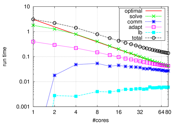
Figure 5: Strong scaling results for 3d Euler shock-interaction problem on a small size computer cluster. The macro grid contains $4\,096$ hexahedrons which is also the coarsest grid and the maximal refinement level is set to $4$ (parameter $22\ 0\ 4$).

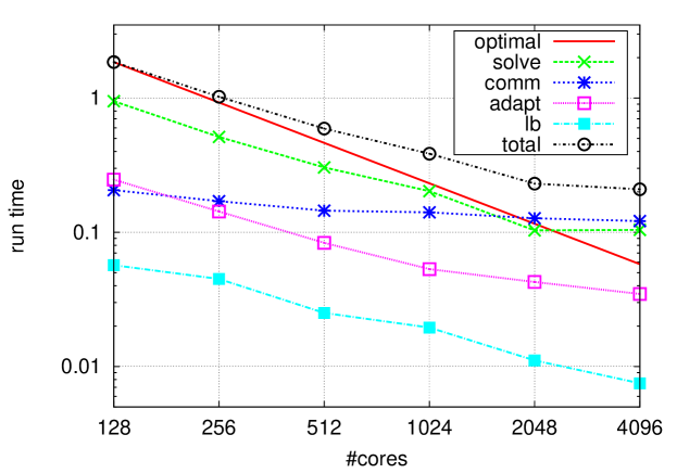
Figure 6: Strong scaling results for Euler shock-interaction problem on the peta scale supercomputer Yellowstone [1]. The macro grid contains $32\,768$ hexahedrons which is also the coarsest grid and the maximal refinement level is set to $6$ (parameter $23\ 0\ 6$).

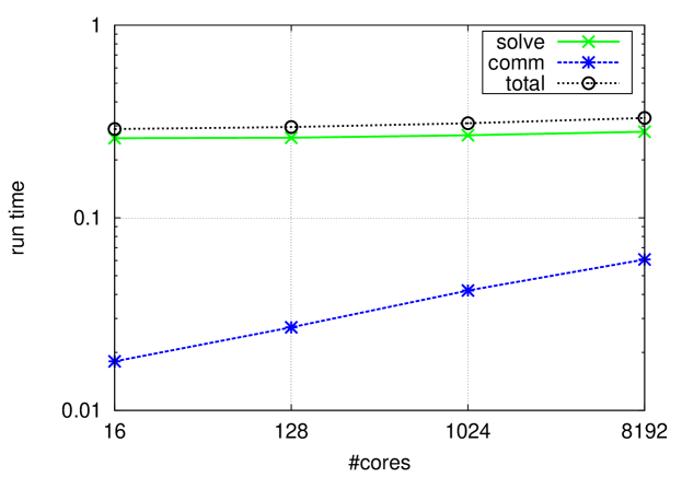
Figure 7: Weak scaling results for Euler shock-interaction problem on the peta scale supercomputer Yellowstone [1]. The number of elements is kept constant per core at $131\,072$ hexahedrons (parameter $25\ 2\ 0$).

3 Using the DUNE-ALUGrid Module

This section discusses the features of Dune-ALUGrid from a user perspective. Special emphasis will be put on extensions to the Dune grid interface.

3.1 Structure of the Module

The structure of the new module is as follows: the main code for the grid implementation and the Dune bindings are in the dune folder of the Dune-ALUGrid module. A program to read in a macro grid on a single processor and to write a partitioned version in a binary format to a file is provided in the utility folder. Finally the examples folder contains the main executables for testing the Dune-ALUGrid modules. All the test problems can be used with any grid manager implementing the Dune-Grid interface. This makes it not only possible to test the ALUGrid implementation but also to compare with other realizations of the Dune grid interface. The code is very similar to the example provided in the Dune-Fem-Howto and comparable with the tutorial found in the Dune-Grid-Howto.

The code is mainly distributed across four files;

main.cc

contains the initial grid construction and the time loop.

fvscheme.hh

contains the computation of the update vector and the marking strategy.

adaptation.hh

contains the code for carrying out the grid modification.

piecewisefunction.hh

contains all classes used to handle the degrees of freedom including storage, restriction and prolongation, and communication.

Switching between the three different test cases is done via pre-processor flags or by making one of the three executables main_ball , main_transport , or main_euler . Each program takes three command line parameters:

  ./main [problem-nr] [startLevel] [maxLevel]

The first one determines the test case to use (including initial data and macro grid); startLevel and maxLevel determine the coarsest and finest grid level, respectively.

Extensions of the Dune grid interface discussed in this paper can be tested in different sub-folders of examples . The basic code is always the same with the necessary changes described in detail in the following chapters. There are four sub-folders, each containing a script, to compare the original and the modified implementation. Again, pre-processor defines are used to provide different implementations in the same code:

callback

compare dof storage and callback adaptation in serial.
Script: check-adaptation.sh
Pre-processor flags: CALLBACK and USE_VECTOR_FOR_PWF .

communication

test asynchronous communication with callback adaptation and persistent container (best from before)
Script: check-communication.sh
Pre-processor flags: NON_BLOCKING .

loadbalance

test the extensions to the loadbalancing interface. In addition to the internal loadbalancing methods, user-defined weights can be added (preprocessore flag USE_WEIGHTS and a simple user-defined loadbalancing strategy is available (flag USE_SIMPLELB . With the flag USE_ZOLTAN a complete reimplementation of the internal zoltan bindings is available based on the extensions of the grid interface (requires the configure option enable-experimental-grid-extensions ).

testEfficiency

test on one computer using multi-core, e.g. $1\to 2\to 4\to 8$, and test on cluster with N computers and P cores, e.g., $P\to 2P\to 4P\to 8P$. By changing the pre-processor flags in the script different versions can be tested.
Script: check-efficiency.sh
Pre-processor flags: CALLBACK , USE_VECTOR_FOR_PWF , NON_BLOCKING .

Note that by default the cube version of Dune-ALUGrid is used. This can be changed in Makefile.am .

3.2 Configuration

The new Dune-ALUGrid module is available via the module home page http://users.dune-project.org/projects/dune-alugrid. The repository can be accessed using the git repository from https://users.dune-project.org/repositories/projects/dune-alugrid.git.

The Dune-ALUGrid module depends on Dune-Grid and can be easily configured using the Dune build system. Using Dune-ALUGrid in a user module then only requires adding a dependency (or suggestion) in the dune.module file, including dune/alugrid/grid.hh , and using

Dune::ALUGrid¡ dimgrid, dimworld, eltype, refinetype, communicator ¿

with $2\leq$ dimgrid $\leq$ dimworld $\leq 3$ for grid and world dimension, eltype $=$ Dune::simplex , Dune::cube , and refinetype $=$ Dune::conforming , Dune::nonconforming . In this version, the only restriction is that conforming refinement is not a valid choice for cube grids. Contrary to previous versions, conforming refinement for a 3d simplex grid is now available. For the communicator, either ALUGridMPIComm for a parallel grid or ALUGRIDNoComm for serial grid can be used. By default, MPI communication is used, if available. Note that if Dune-ALUGrid was compiled in parallel mode then MPI has to be initialized before constructing a grid object even in a serial computation.

There are a number of packages which can be used to increase the flexibility and performance of the Dune-ALUGrid module. Paths to the installed versions of these packages have to be provided during the configuration of the module, i.e., within the configuration file used in the call of the dunecontrol script:

--with-dlmalloc=PATH:

path to Doug Lea’s malloc library (required version $>=2.8.6$). If this library is available the memory management for Dune-ALUGrid will use the dlmalloc package [26]. This can improve performance as shown in Section 2.1.

--with-metis=PATH:

path to the Metis library [19]. If available, Metis can be used for load balancing.

--with-metis-lib=NAME:

name of the metis libraries (default is metis ).

--with-zoltan=PATH:

path to the Zoltan package. This package provides a wide range of additional load balancing methods including those provided by Metis and ParMetis. Details on how to use different load balancing methods are provided in Section 3.7.

--with-zlib=PATH:

path to zlib [17]. If available, zlib compression can be used for backup and restore of a full Dune-ALUGrid grid object. More details on data I/O are provided in Section 3.4.

3.3 Parallel Grid Construction

Any grid-based numerical simulation must at some time construct a grid of the computational domain. The general Dune grid interface assists this step by providing three basic construction mechanisms:

GridFactory

is a general interface for the construction of unstructured grids. Basically, it constructs the grid from a list of vertex coordinates and a list of elements.

StructuredGridFactory

can be used to construct a grid of an axis-aligned cube domain. For unstructured grids, a default implementation based on the GridFactory is provided.

GridReaders

can be used to read files given in a special format. These readers will generally use the GridFactory to construct the grid. A Dune specific format is available through the DGF reader. An extension of this format to partitioned grids is discussed in Section 3.3.3.

Additionally, Dune-ALUGrid provides a native file format for predistributed macro grids.

At the time of this writing, the GridFactory interface does not support the construction of unstructured grids in parallel. The entire grid must first be constructed on one process and then distributed to all processes using the load balancing algorithm. For large macro grids, this method is at least inefficient if not impossible as the macro grid might not even fit into the memory of one computational node. Without specialization, this restriction also holds for the StructuredGridFactory and the DGF parser. Dune-ALUGrid overcomes this difficulty by providing specializations of all three grid construction mechanisms. In addition the Dune-ALUGrid module contains utility tools to perform the distribution off line, writing native distributed ALUGrid files for use in the actual computation. These will be described at the end of this section.

3.3.1 The GridFactory

In Dune, the construction of unstructured grids is handled by the GridFactory class, which has to be specialized for each grid implementation supporting them. The most important interface methods are

⬇

void insertVertex ( const Dune::FieldVector<ctype,dimensionworld> &coord );

void insertElement( const Dune::GeometryType &type,

const std::vector<unsigned int> &vertices );

void insertBoundarySegment( const std::vector<unsigned int> &vertices );

The main difficulty when constructing a predistributed grid is the identification of the process boundaries. Using a large amount of global communication and coordinate comparison this could be achieved using the interface provided by the Dune-Grid module. Since this is neither efficient nor very reliable, we extend the interface requiring the user to provide a globally unique number for each vertex in the macro grid using the method:

⬇

void insertVertex ( const Dune::FieldVector<ctype, dimensionworld> &coord,

VertexId globalId );

This unique numbering is sufficient to use the grid factory concept in parallel. Notice that elements and boundaries are inserted using a local vertex number corresponding to the insertion order. VertexId in the current implementation is an unsigned integer.

To further increase efficiency, faces on process boundaries can also be inserted, reducing the need for global communication during grid construction. Similar to the insertBoundarySegment method, the grid factory in Dune-ALUGrid allows the insertion of process borders through the method

⬇

void insertProcessBorder ( const std::vector<unsigned int> &vertices );

While it is not necessary to insert process borders, we strongly recommend doing so, because the construction of this information within the grid factory requires an expensive global communication. Note that this method will not work accurately, if it is called for some process borders only.

In some cases it is easier to simply insert into the factory that a certain face of an element is on the border or on the boundary (see the example in Section 3.3.2). The grid factory in Dune-ALUGrid allows this through the following methods:

⬇

void insertBoundary ( int element, int faceInElement );

void insertProcessBorder ( int element, int faceInElement );

The local face numbering used for faceInElement corresponds to the Dune reference element.

3.3.2 StructuredGridFactory

An example of how to use the new methods on the grid factory to construct a distributed grid is provided in the specialization of the StructuredGridFactory in dune/alugrid/common/structuredgridfactory.hh .

Given an interval $[a,b]\subset\mathbb{R}^{3}$ and a subdivision vector $N\in\mathbb{N}^{3}$, a distributed Cartesian grid is constructed. Each process first uses SGrid (a structured grid manager available in Dune-grid) to setup a Cartesian grid. A space filling curve is then used to partition this grid and the distributed grid is constructed using the extended grid factory of Dune-ALUGrid on each process. Note that the resulting partition on each process does not consist of a product of intervals, since the distribution is done using a space filling curve.

The following code snippet shows the idea in a very general setting. The gridView object is the leaf grid view of a given grid (e.g. of a SGrid ), indexSet denotes its index set, and the partitioner object provides a method rank(const Entity &) returning the MPI rank that the entity shall be assigned to (e.g. based on a space filling curve).

⬇

//create ALUGrid GridFactory

GridFactory< Grid > factory;

//map global vertex ids to local ones

std::map< IndexType, unsigned int > vtxMap;

const int numVertices = (1 << dim);

std::vector< unsigned int > vertices( numVertices );

int nextElementIndex = 0;

const auto end = gridView.template end< 0 >();

for( auto it = gridView.template begin< 0 >(); it != end; ++it )

{

const Entity &entity = *it;

if( partitioner.rank( entity ) != myrank )

continue;

//insert vertices and element

const typename Entity::Geometry geo = entity.geometry();

for( int i = 0; i < numVertices; ++i )

{

const IndexType vtxId = indexSet.subIndex( entity, i, dim );

auto result = vtxMap.insert( std::make_pair( vtxId, vtxMap.size() ) );

if( result.second )

factory.insertVertex( geo.corner( i ), vtxId );

vertices[ i ] = result.first->second;

}

factory.insertElement( entity.type(), vertices );

const int elementIndex = nextElementIndex++;

const auto iend = gridView.iend( entity );

for( auto iit = gridView.ibegin( entity ); iit != iend; ++iit )

{

const Intersection &isec = *iit;

const int faceNumber = isec.indexInInside();

//insert boundary face in case of domain boundary

if( isec.boundary() )

factory.insertBoundary( elementIndex, faceNumber );

//insert process boundary if the neighboring element has a different rank

if( isec.neighbor() && (partitioner.rank( *isec.outside() ) != myrank) )

factory.insertProcessBorder( elementIndex, faceNumber );

}

}

3.3.3 Dune Grid Format (DGF)

The DGFParser has also been extended to make use of the parallel grid construction available in Dune-ALUGrid. For each process a dgf file (e.g., grid.dgf.P.1 , …, grid.dgf.P.P ) is used containing only one part of the grid. As in the serial case the blocks with the information on the elements uses a process local numbering of the vertices. A new block GlobalVertexIndex has to be added, where a globally unique integer for each vertex in this partition is provided in the same order used for the coordinates in the Vertex block. The file passed to the GridPtr class (e.g. grid.dgf.P ) contains only the block ALUParallel listing the file names of the individual partitions for each process.

The following shows an example for the domain $[0,1]^{3}$ divided into $4$ elements and distributed over two processors:

cube.dgf.2	cube.dgf.2.1	cube.dgf.2.2
⬇ DGF VERTEX 0.5 0 0 1 0 0 0.5 0.5 0 1 0.5 0 0.5 0 1 1 0 1 0.5 0.5 1 1 0.5 1 0.5 1 0 1 1 0 0.5 1 1 1 1 1 # CUBE 0 1 2 3 4 5 6 7 2 3 8 9 6 7 10 11 # GLOBALVERTEXINDEX 1 8 3 9 5 10 7 11 13 16 15 17 #

These files were generated by using the utility ParallelDGFWritter class (in dune/alugrid/common/writeparalleldgf.hh ) to provide distributed dgf files from a given input dgf file.

3.3.4 Utility programs

The Dune-ALUGrid module also provides an utility program utils/convert-macrogrid/convert to convert a normal DGF file or a legacy ALUGrid macro grid file into Dune-ALUGrid’s new binary or compressed binary macro grid file format. This tool can also decompose the macro grid into several partitions. Dune-ALUGrid is able to read decomposed macro grids if the number of partitions of the macro grid is smaller or equal to the used number of cores. This is especially useful for very large macro grids which will not fit into the memory of a single core. In addition the compressed binary format reduces storage requirements and decreases storage access times.

3.4 Backup and Restore

For backup and restore as it is needed for checkpointing and postprocessing a new interface was recently introduced into Dune-Grid. To our knowledge Dune-ALUGrid is the first grid manager implementing this interface so we will go into a bit more detail in the following. The interface is given by

⬇

template< int dim, int dimworld,

ALUGridElementType elType,

ALUGridRefinementType refineType, class Comm >

struct BackupRestoreFacility<

ALUGrid< dim, dimworld, elType, refineType, Comm > >

{

/** perform backup of grid to given std::ostream*/

static void backup ( const Grid &grid, std::ostream &stream ) ;

/** restore grid from std::istream and return pointer to newly created grid object*/

static Grid* restore ( std::istream &stream ) ;

};

The BackupRestoreFacility provides two further backup and restore methods where a filename is the argument instead of a stream. These methods have been added for legacy codes like ALBERTA [31] that might not support the read and write via streams. For Dune-ALUGrid these are simply implemented using a file stream and the calling the above mentioned methods.

For data I/O on large parallel machines we provide two mechanisms. The conventional approach is to use standard file streams to create a binary file for each process containing the macro grid cells, refinement tree, and index information for the corresponding partition. This becomes very cumbersome when the code is used with many cores. Therefore, the second approach is to use a std::stringstream to write all information into a buffer of type char* and then use a library like SIONlib [16] to write the data to the storage unit. This approach has the advantage that libraries like SIONlib provide the maximal I/O performance but do not limit Dune-ALUGrid to be used only with this library. For libraries that require the size of data to be written, like SIONlib, the intermediate storage in a char buffer is necessary since for the adaptive grid the number elements is not known apriori. How SIONlib is used is shown in the examples presented in examples/backuprestore . This example explains how backup/restore is done using different ways to write data to the storage device.

Note that Dune-ALUGrid will only backup/restore it’s LocalIdSet . The GlobalIdSet is generated from the unique macro element id (built from the unique vertex ids) and the position in the refinement tree and therefore does not need to be stored explicitly. Furthermore, the persistent order of the macro grid automatically induces the same traversal order for the hierarchical grid. Since both, the LevelIndexSet and the LeafIndexSet are generated by grid traversal and insert on first visit strategy, both index set variants preserve their indices over a backup and restore process.

3.5 Overlapping Communication and Computation

In a numerical algorithm, degrees of freedom are typically attached to grid entities. Now, a single grid entity can be visible to multiple processes and any data attached to it needs to be synchronized between these processes. The Dune grid interface therefore requires each grid view to support this synchronization through a communicate method:

⬇

template< class DataHandle >

void communicate ( DataHandle &, InterfaceType,

CommunicationDirection ) const;

The interface type and communication direction specify the set of entities on which data has to be sent or received. On the sending side the data handle is responsible for packing entity data into a buffer; on the receiving side it unpacks the data again. The actual data transfer is done transparently by the grid implementation.

After all data has been sent, the grid implementation has to wait until incoming data is received, which can be a waste of valuable computation time. Indeed, many numerical algorithms can be split into work that depends on the shared data and work that does not. The latter part can actually be done while communication is in progress simply by splitting sending and receiving in two parts and is supported even by the oldest MPI implementations.

To make use of the valuable communication time, Dune-ALUGrid allows to delay the receiving process to a convenient point in the algorithm. The actual communication initiated by communicate becomes an object:

⬇

template< class DataHandle >

Communication< DataHandle > communicate ( DataHandle &, InterfaceType,

CommunicationDirection ) const;

Such a Communication object satisfies the following interface:

⬇

struct Communication

{

//wait for communication to finish if not already done

~Communication () { if( pending() ) wait(); }

//is this communication still pending?

bool pending () const;

//wait for communication to finish

void wait ();

};

While the communication is pending, i.e., while wait has not been called, the reference to the data handle must remain valid. As wait is automatically called in the destructor, ignoring the return value will result in a blocking communication. Thus no change is required to existing code if blocking communucation is to be used.

If gridView is a grid view of an ALUGrid object, overlapping communication and computation is rather simple:

⬇

//construct data handle for the communication

auto comm = gridView.impl().communicate ( dataHandle, interface, dir );

//do some computation not depending on the remote data

comm.wait();

// do computation depending on the remote data

Note that the method impl is only available if experimental grid extensions have been enabled in Dune-Grid and would no longer be required once the new interface is added into Dune-Grid.

A possible usage of the communication hiding is presented in the following code snippet. The method is implemented in examples/communication where the main change in the time loop is quite simple:

⬇

//original non-blocking code: dt = scheme( time, solution, update ) ;

{

//new code: compute data on border and ghost entities

dt = scheme.border( time, solution, update );

//start non-blocking communication

auto commObject = grid.communicate( handle, interface, direction );

//do computation not depending on remote data

dt = std::min(dt , scheme( time, solution, update ) );

} // communication will be finished when commObject goes out of scope

3.6 Adaptation Using Call-Backs

Grid modification in Dune is performed in three steps. First grid.preadapt() is called to start the modification phase. After this method has been called the index sets are no longer valid and data has to be accessed based either on one of the IdSets or using a PersistentContainer . Both allow storage of data persistently during grid modification and on the whole hierarchy of the grid making it possible for data to be restricted and prolongated from one level to another. Next grid.adapt() is called which refines or coarsens grid elements according to markers set by the user. Finally grid.postadapt() is called, ending the modification phase and reinitializing the Dune consecutive, zero starting index sets allowing to store user data in consecutive memory locations.

The main steps for the user consist in making data persistent during the modification stage of the grid, prolongation of data if elements are refined, and restriction of data if elements are coarsened. A common approach is to store the data in a vector-like structure in the computation phase for efficient memory access. The necessary copying of the data into a PersistentContainer during the modification phase makes this step computationally more expensive. Alternatively, the user can store data directly in a PersistentContainer which means that the storage does not have to be modified during grid changes but sacrificing efficiency during the computation phase due to more expensive data access. In Dune the PersistentContainer can be specialized for each grid implementation. A default implementation uses a std::map to store the data using the LocalIdSet of the grid as key. Dune-ALUGrid uses a speciallization of this class based on a std::vector to store the data. Each entity stores an integer which is unique within the grid hierarchy and which can be used to access the data within the vector. In contrast to a Dune IndexSet this index is not necessarily zero starting and consecutive, resulting in holes within the PersistentContainer but allowing for a constant retrieval time of the data. In our example adaptive Finite Volume scheme the two storage strategies are available for testing. By default the PersistentContainer is used but by defining USE_VECTOR_FOR_PWF the degrees of freedom will be stored in a vector-like structure and moved into a PersistentContainer only during the grid modification stage. In all our tests the storage of data in the PersistentContainer was significantly more efficient. Some results are shown in the Dune columns of Table 2.

In addition to the approach described above, Dune-ALUGrid provides an adaptation mechanism using a callback approach, similar to the Dune communication and loadbalancing interface (see Section 3.7). Instead of the grid.preAdapt() , grid.adapt() , grid.postAdapt() algorithm, a single call to grid.adapt( dataHandle ) is required. The dataHandle has to be derived from

⬇

template< class Grid, class Impl >

struct AdaptDataHandle

{

typedef typename Grid::template Codim< 0 >::Entity Element;

void preCoarsening ( const Element &father );

void postRefinement ( const Element &father );

};

The method preCoarsening is called on the element father before all its descendants are removed. Accordingly, the method postRefinement is called immediately after descendants for an entity father are created. Since these methods are called during grid modification the IndexSets on the grid are not available and data has to be stored in some peristent manner, e.g., using the PersistentContainer . There is no need to call preAdapt(),postAdapt() on the grid.

This variant of the adaptation cycle is implemented in examples/callback/adaptation.hh . Assuming that the degrees of freedom are stored in a PersistentContainer one simply needs to call

⬇

grid_.adapt( *this );

and implement the two callback methods

⬇

void preCoarsening ( const Entity &father )

{

Container &container_ = getSolution().container();

//average the data from all children and copy onto the father entity

Vector::restrictLocal( father, container_ );

}

//called when children of father where newly created

void postRefinement ( const Entity &father )

{

Container &container_ = getSolution().container();

container_.resize();

//copy the data from the father onto all its children

Vector::prolongLocal( father, container_ );

}

The results of using the callback approach are shown in the corresponding columns of Table 2. In summary, our tests indicate a gain of up to $10\%$ using callback adaptation. In addition the overall implementation is simpler since the hierarchic restriction and prolong methods do not have to be implemented. To run the test described here go to the examples/callback directory and run the check-adaptation.sh script. The implementation with a PersistentContainer is also compared here with the version based on vector-like structure. The advantage of using a PersistentContainer for the degrees of freedom in the Finite Volume scheme is significant (more than $20\%$).

Table 2: Results for callback adaptation and dof storage strategy obtained on a single core from our small cluster. See script examples/callback/check-adaptation.sh . T stands for transport problem and E for Euler problem, followed by the three program parameters used.

storage		vector	vector	PersistentContainer	PersistentContainer
adaptation		Dune-	callback	Dune-	callback
T	2 0 2	251s	227s	194s	173s
T	2 0 3	2411s	1820s	2222s	1647s
E	21 0 3	106s	83s	99s	77s
E	21 0 4	1070s	1037s	833s	766s

3.7 Internal Load Balancing

There are two stages in a computation where load balancing is essential in a simulation. During the start up phase of the computation where the grid has to be distributed over the available number of processes and after the grid has been locally refined. Even if the grid has been partitioned beforehand and Dune-ALUGrid’s parallel grid factory is used, it is still sometimes of practical interest to repartition the grid after creation, e.g., if a larger number of processes are available for the computation. To this end the Dune-Grid interface provides the method

⬇

bool loadBalance();

Even if the initial grid is optimally distributed, the load can become unbalanced during the computation for example if local adaptivity is used. In this case the method mentioned above is not sufficient as it does not allow to migrate user data together with elements from one process to another. To manage data migration the Dune-Grid interface provides a second method

⬇

template< class DataHandleImpl, class Data >

bool loadBalance( CommDataHandleIF< DataHandleImpl, Data > &dataHandle );

The handling of user data is achieved by a callback mechanism using the same interface used for communication during the computation. Basically, for each element to be removed on the given process a method gather is called (to collect data to be shipped with the element) and when a new element is added to the grid on the process then a method scatter is called (to deliver the data that was shipped with the element ) on the dataHandle instance.

The main problem with these two methods is that there is no mechanism for the user to intervene with the details of partitioning computed by the grid manager. This new module provides two mechanisms for the user to improve the internal load balancing to suit the need of the application at hand. Before presenting these improvements, we give a brief description of how Dune-ALUGrid’s internal load balancing strategy works.

Dune-ALUGrid only allows for horizontal load balancing, i.e., partitioning of the elements on the macro level, migrating the whole tree below a given macro element from one process to another. Each macro element $E$ is assigned a weight equal to the number of leaf elements below $E$. Using these weights either a space filling curve approach is used or a graph partitioning algorithm is used. In ALUGrid 1.52 only serial graph partitioning using the Metis library [19] could be used. The serial graph partitioning requires the communication of the whole assembled graph to all processes which does not scale in terms of memory and communication time. While this method can still be used in Dune-ALUGrid, additional bindings to Zoltan [8] have been added (providing space filling curve and graph partitioning methods). Via the Zoltan interface ParMetis [30] is available as well. The graph is constructed using the weighted macro elements as nodes and connecting neighboring macro elements $E_{1},E_{2}$ with an edge in the graph. These edges are assigned weights according to the number of leafs below $E_{1},E_{2}$ which are neighbors. The node weights are to represent the computational cost, while the edge weights represent the communication size in the case that these elements come to be on different processors. The newly implemented partition algorithm for space filling curves makes Dune-ALUGrid more self contained. As a default we are using the Hilbert space filling curve (see for example [3]) provided by Zoltan [8]. The element weights described above are used to determine the optimal partitioning of the space filling curve. Besides the space filling curve based approach provided by Zoltan called HSFC (id 13) Dune-ALUGrid also provides it’s own load distribution algorithm. In this case it is assumed that the elements of the macro mesh are sorted by a space filling curve. Then the distribution of the load boils down to the distribution of a 1d graph with attached weights. If Zoltan is available and no pre-ordered mesh is provided, the Hilbert space filling curve from the Zoltan package is used to sort the elements. As a fallback Dune-ALUGrid also provides it’s on implementation based on the Z-curve (aka Morton curve) approach. The algorithm to partition the 1d graph is based on the one described in [11, Algorithm 16] with some slight modifications such as avoiding empty partitions in any case if the number of macro elements is larger than the number of cores used. Dune-ALUGrid’s internal space filling curve with linkage (id 4) algorithm comes with a further advantage: The communication after a redistribution to identify master-slave node relations can be done without communication. In all other cases listed in Table 3 an all-to-all communication is needed to compute the master-slave relation of vertices that are present on multiple cores.

The simplest way to tweak the internal load balancing algorithm are three parameters read from a file called alugrid.cfg , which is searched for in the current working directory. This file has to contain three values. The fist two numbers ( lbUnder , lbOver ) in the alugrid.cfg file allow to specify a certain amount of load inbalance which has to be exceeded before the partitioning is adjusted. A new partitioning is computed only if the maximum number of leaf elements in a partition exceeds lbOver times the mean number of elements or the minumum number is smaller than lbUnder times the mean number of elements in all partitions. The third value is an integer between $0$ and $15$ determining the partitioning method to use. Table 3 gives an overview of available methods and their numbering.

Table 3: Internal partitioning methods and corresponding id.

method name	id	method name	id
NONE	0	COLLECT (to rank $0$)	1
Space Filling Curve (linkage)	4	Space Filling Curve	9
METIS (PartGraphKway)	11	METIS (PartGraphRecursive)	12
ZOLTAN (HSFC)	13	ZOLTAN (GRAPH)	14
ZOLTAN (PARMETIS)	15

A second option to influence the outcome of the load balancing algorithm is to provide other weights for the elements (i.e., the graph nodes). This can improve the overall effciency of a scheme if the number of leaves does not directly represent the computational cost associated with a given macro element. An example for this are reactive flow problems where substepping in time is used to resolve stiff sources locally on each element [18]. Further examples are the solution of PDEs in a moving domain [24] or a multi-domain approach where partial differential equations with different complexity are solved in different domains represented on the same underlying grid [29]. The corresponding additional methods are

⬇

template< class LBWeights >

bool loadBalance ( LBWeights &weights );

template< class LBWeights, class DataHandleImpl, class Data >

bool loadBalance ( LBWeights &weights,

CommDataHandleIF< DataHandleImpl, Data > &dataHandle );

LBWeights must implement int operator()(const Grid::Codim¡0¿::Entity &) which will be called for each macro element to provide the weight, here an integer value. An example usage is shown in examples/loadbalancing/loadbalance_simple.hh . Each leaf element is assumed to carry a computational cost of $2^{l}$ where $l$ is the level of the leaf element. The weight for a macro element is then simply the sum of the weights over all underlying leaf elements.

In Figure 8, 9, 10, and 11 we present a comparison of the different load balancing algorithms available in Dune-ALUGrid. The results show a strong scaling study using the ball example with refinement as described in (1). The scaling studies have been carried out on Yellowstone [1].

In Figure 8 we present a comparison of run times for ALUGrid’s $1.52$ version and the new Dune-ALUGrid module. Since in version $1.52$ only Metis was available for partitioning we only compare the run times using the Metis partitioning. We discover that both the tetrahedral and the hexahedral version perform better in the new Dune-ALUGrid implementation.

For the comparison of load balancing methods in Figure 9, 10, and 11 we can see that the space filling curve approaches, either Dune-ALUGrid’s internal methods or the HSFC method from Zoltan, perform best even if the macro grid does not allow a good partitioning anymore because the average element per core ratio is very small. The graph partitioning methods are in general more expensive even though the created partitions seem to be more efficient in terms of communications effort resulting in faster run times for the adaptation step (see Figure 9b, 10b, and 11b). As a drawback all tested graph partitioning methods fail when the number of elements per core becomes very small. We have to point out that this example is heavily communication based and especially the load balancing step, which is done in every time step, is very communication intensive. So it seems even more impressive that the run times still drop when using $2048$ or $4096$ cores. This is confirmed by a comparable study in [35] where a stagnation in strong scaling was observed when adaptivity and load balancing was done every time step. As a conclusion the space filling curve approaches seem more suitable for problems with frequent redistribution of the mesh whereas the graph partitioning methods seem more favorable for productions runs on a fixed non-adaptive grid.

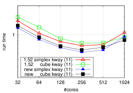
(a) overall

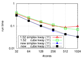
(b) adaptation

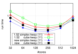
(c) load balancing

Figure 8: Comparison of ALUGrid $1.52$ and Dune-ALUGrid using the ball example with a macro mesh of $32\,768$ hexahedrons or $196\,608$ tetrahedrons. The grid is refined uniformly once and the maximal refinement level is $4$ (parameter 3 1 4 for example main_ball ). Here, we only use the METIS PartGraphKway (partition method id 11) method for domain decomposition.

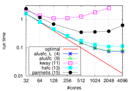
(a) overall

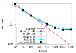
(b) adaptation

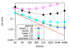
(c) load balancing

Figure 9: Strong scaling of the ball example from equation (1) using a conforming simplex grid with a macro mesh containing $196\,608$ tetrahedrons. The grid is refined uniformly once and the maximal allowed refinement level is $4$ (parameter 3 1 4 for example main_ball ). The graphs show the average run time per time step of different parts of the algorithm.

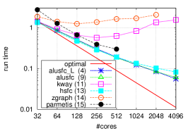
(a) overall

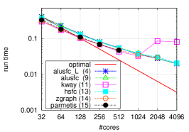
(b) adaptation

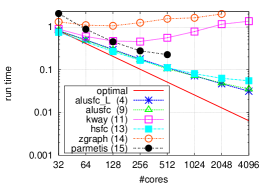
(c) load balancing

Figure 10: Strong scaling of the ball example from equation (1) using a non-conforming cube grid with a macro mesh containing $32\,768$ hexahedrons. The grid is refined uniformly once and the maximal allowed refinement level is $4$ (parameter 3 1 4 for example main_ball ). The graphs show the average run time per time step of different parts of the algorithm.

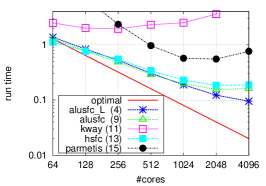
(a) overall

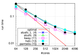
(b) adaptation

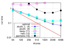
(c) load balancing

Figure 11: Strong scaling of the ball example from equation (1) using a non-conforming cube grid with a macro mesh containing $262\,144$ hexahedrons. The maximal allowed refinement level is $3$ (parameter 4 0 3 for example main_ball ). The graphs show the average run time per time step of different parts of the algorithm.

3.8 User Defined Partitioning

A more general approach is provided by the methods

⬇

template< class LBDestinations >

bool repartition ( LBDestinations &destinations );

template< class LBDestinations, class DataHandleImpl, class Data >

bool repartition ( LBDestinations &destinations,

CommDataHandleIF< DataHandleImpl, Data > &dataHandle);

performing load balancing either without or with migrating user data using callback on the dataHandle instance. Otherwise, the whole load balancing is taken care of by the user. The class LBDestinations has to fulfill the following interface

⬇

struct LBDestinations

{

//Return process number the given macro element should be assigned to.

int operator()(const Grid::Codim<0>::Entity &);

//Fill set of ranks the current process will receive elements from and return true

//in this case. If false is returned, then ALUGrid will compute this information

//via a global communication.

bool importRanks( std::set<int>& ranks ) const;

};

where the int operator()(const Grid::Codim¡0¿::Entity &) returns the process number an element is to be moved to. In Dune-ALUGrid this method will be called for each macro element on the given rank and that macro element together with all its children will be moved to the desired partition. The method importRanks can simply return false and then does not need to fill the set ranks . However, this decreases performance due to the global communication required to find out from which ranks to expect data. Some partitioning tools like Zoltan provide this information, so that the user only needs to copy it to ranks vector and return true to improve parallel efficiency.

An example usage is shown in examples/loadbalancing/loadbalance_simple.hh . The partitioning is computed by keeping the center on process zero and distributing the rest of the grid in equal slices to the other processors. The only changes required to the algorithm are in main.cc and adaptation.hh where the calls of the loadbalance(…) method on the grid are replaced with the new repartition(…) methods In each step of the scheme before calling grid.repartition(…) the method repartition() is called on the loadbalance handle. This causes an internal variable to be increased, leading each time to a new partitioning:

⬇

template< class Grid >

struct SimpleLoadBalanceHandle

{

typedef SimpleLoadBalanceHandle This;

typedef typename Grid :: Traits :: template Codim<0> :: Entity Element;

SimpleLoadBalanceHandle ( const Grid &grid )

: angle_( 0 )

, maxRank_( grid.comm().size() )

{}

/** this method is called before invoking the repartition method on the grid, to check if the user-defined partitioning needs to be readjusted*/

bool repartition ()

{

angle_ += 2.*M_PI/50.;

return true;

}

/** This is the method, called from the grid for each macro element. It returns the rank to which the element is to be moved.*/

int operator()( const Element &element ) const

{

typedef typename Element::Geometry::GlobalCoordinate Coordinate;

Coordinate w = element.geometry().center();

w -= Coordinate(0.5);

if (w[0]*w[0]+w[1]*w[1] > 0.1 && maxRank_>0)

{ //distribute everything away from the center in equal slices

double phi=arg(std::complex<double>(w[0],w[1]));

if (w[1]<0) phi+=2.*M_PI;

phi += angle_;

phi *= double(maxRank_-1)/(2.*M_PI);

int p = int(phi) % (maxRank_-1);

return p+1;

}

else //keep the center on proc 0

return 0;

}

/** This method can simply return false, in which case ALUGrid will internally compute the required information through some global communication. To avoid this overhead the user can provide the ranks of partitions from which elements will be moved to the calling repartition.*/

bool importRanks( std::set<int> &ranks) const { return false; }

private:

double angle_;

int maxRank_;

};

A more useful example is given in examples/loadbalancing/loadbalance_zoltan.hh , where the algorithm in Dune-ALUGrid relying on the Zoltan’s graph partitioner is replicated using the Dune interface. Note that the results will not be identical since the order of the edges within the graph will differ slightly when using the Dune interface to build it. Nevertheless, the algorithm and parameter settings for Zoltan are identical. Based on this implementation it is easy to experiment with the wide range of options Zoltan provides to optimize the partitioning algorithm for a given application. Note also that the class again contains a repartitioning method using the same lbOver , lbUnder values provided in the alugrid.cfg file.

Constructing the graph relying only on the available Dune interface would be quite cumbersome and involve quite a bit of overhead. There is no direct way to compute the edge weights and the master rank for each ghost element has to be passed on to Zoltan, information requiring an extra communication step within Dune. To simplify constructing the graph Dune-ALUGrid provides a new method on the grid.

⬇

template<PartitionIteratorType pitype>

typename Partition<pitype>::MacroGridView macroView() const;

This method returns a view of the macro grid level of the grid. The MacroGridView contains the usual method to iterate over the macro grid and obtain an index set but in addition includes some useful methods to construct the dual weighted graph:

⬇

//return the master process of the given element

int master ( const typename Codim< 0 > :: Entity &entity ) const;

//return a globally uniqe integer id for this element

int macroId ( const typename Codim< 0 > :: Entity &entity ) const;

//return the weight (number of leaf elements) for the given elements

int weight ( const typename Codim< 0 > :: Entity &entity ) const;

//return the weight for this intersection

int weight ( const Intersection &intersection ) const;

The Zoltan example demonstrates a practical usage of the new load balancing interface and also an extension not directly available using the internal bindings: The hypergraph algorithm of Zoltan can be used to fix a set of elements to a given processor. By changing the variable fix_bnd_ to true the partitioning is computed such that all elements adjacent to left boundary face are kept on process zero throughout the simulation. A practical example of this possibility is discussed in [7]. It should be noted that, although the algorithm used in this example mirrors the one used in the Dune-ALUGrid internal bindings to Zoltan, the results might not be the same. The reason is that iteration order over the macro elements can differ and this results in slightly different dual graphs.

Note: As pointed out above, Dune-ALUGrid only allows to partition the macro level of the grid. Depending on the problem the macro grid might not contain enough elements or the adaptivity might be too localized to allow for a balanced load if only macro elements are distributed. On manycore systems a possible solution is to use fewer processes to distribute the macro grid and use threading to partition directly on the leaf level. This approach has been evaluated in [22].

4 Conclusions

In this paper we briefly described the main new features available in the overhaul of Dune-ALUGrid. The main improvements concern the parallel feature set of the library, including now user-defined load balancing and parallel grid construction as well as a decreased memory footprint. Since ALUGrid is and was widely used within the Dune community we expect that numerous Dune users will benefit from work presented here. We also presented a number of extensions to the Dune grid interface that prove useful and will hopefully be integrated into the Dune grid interface in the near future.

The increased feature set also includes newest vertex bisection for tetrahedral grids in 3d, making it the only parallel grid manager within Dune with this feature. This will enable the usage of conforming adaptive discretization methods, such as conforming adaptive Finite Elements, in parallel. Nevertheless, there are some shortcomings that still have to be resolved in the future.

The 2d code has been parallelized by reformulating it as an extension to the 3d code and it thus also inherited all the major features. The usage is similar to the usage of the 3d code.

4.1 Shortcomings and Outlook

A major drawback of the current implementation is that load balancing is performed solely based on the macro grid. This works fine for many problems where the refinement zones are not too restricted to one area of the domain, but will completely fail for very local refinement regions. As already mentioned the situation can be improved by using a hybrid parallelization approach. But the next major improvement will be the implementation of a more flexible partitioning of elements allowing for partitioning of various sets of elements. Furthermore, the current implementation lacks support for ghost elements when bisection refinement is used. This is hopefully fixed in the near future.

References

- [1] Computational and Information Systems Laboratory. 2012. Yellowstone: IBM iDataPlex System (Climate Simulation Laboratory). Boulder, CO: National Center for Atmospheric Research. http://n2t.net/ark:/85065/d7wd3xhc.
- [2] Th. Albrecht, A. Dedner, M. Lüthi, and Th. Vetter. Finite Element Surface Registration Incorporating Curvature, Volume Preservation, and Statistical Model Information. Comp. Math. Methods in Medicine, 2013, 2013.
- [3] M. Bader. Space-Filling Curves - An Introduction with Applications in Scientific Computing, volume 9 of Texts in Computational Science and Engineering. Springer-Verlag, 2013.
- [4] W. Bangerth, T. Heister, L. Heltai, G. Kanschat, M. Kronbichler, M. Maier, B. Turcksin, and T. D. Young. The deal.ii library, version 8.1. arXiv preprint http://arxiv.org/abs/1312.2266v4, 2013.
- [5] P. Bastian, M. Blatt, A. Dedner, C. Engwer, R. Klöfkorn, R. Kornhuber, M. Ohlberger, and O. Sander. A Generic Grid Interface for Parallel and Adaptive Scientific Computing. Part II: Implementation and Tests in DUNE. Computing, 82(2–3):121–138, 2008. http://www.dune-project.org.
- [6] P. Bastian, M. Blatt, A. Dedner, C. Engwer, R. Klöfkorn, M. Ohlberger, and O. Sander. A Generic Grid Interface for Parallel and Adaptive Scientific Computing. Part I: Abstract Framework. Computing, 82(2–3):103–119, 2008. http://www.dune-project.org.
- [7] T. Betcke, A. Dedner, D. Holder, M. Jehl, and R. Klöfkorn. A Fast Parallel Solver for the Forward Problem in Electrical Impedance Tomography. Trans. Bio. Med. Eng., 2014. (accepted).
- [8] E. G. Boman, U. V. Catalyurek, C. Chevalier, and K. D. Devine. The Zoltan and Isorropia parallel toolkits for combinatorial scientific computing: Partitioning, ordering, and coloring. Scientific Programming, 20(2), 2012. http://www.cs.sandia.gov/zoltan/.
- [9] S. Brdar, M. Baldauf, A. Dedner, and R. Klöfkorn. Comparison of dynamical cores for NWP models: comparison of COSMO and DUNE. Theoretical and Computational Fluid Dynamics, 27(3-4):453–472, 2013.
- [10] A. Burri, A. Dedner, R. Klöfkorn, and M. Ohlberger. An efficient implementation of an adaptive and parallel grid in dune. In E. Krause et al., editor, Computational Science and High Performance Computing II, volume 91, pages 67–82. Springer, 2006.
- [11] C. Burstedde, L.C. Wilcox, and O. Ghattas. p4est: Scalable algorithms for parallel adaptive mesh refinement on forests of octrees. SIAM Journal on Scientific Computing, 33(3):1103–1133, 2011. http://www.p4est.org/.
- [12] A. Dedner and R. Klöfkorn. A Generic Stabilization Approach for Higher Order Discontinuous Galerkin Methods for Convection Dominated Problems. J. Sci. Comput., 47(3):365–388, 2011.
- [13] A. Dedner, C. Rohde, B. Schupp, and M. Wesenberg. A parallel, load balanced MHD code on locally adapted, unstructured grids in 3D. Comput. Vis. Sci., 7(2):79–96, 2004.
- [14] B. Faigle. Adaptive modelling of compositional multi-phase flow with capillary pressure. PhD thesis, Universität Stuttgart, 2014. http://elib.uni-stuttgart.de/opus/volltexte/2014/9068/.
- [15] A. Fallahi and B. Oswald. The element level time domain (eltd) method for the analysis of nano-optical systems: Ii. dispersive media. Photonics and Nanostructures - Fundamentals and Applications, 10(2):223 – 235, 2012.
- [16] W. Frings, F. Wolf, and V. Petkov. Scalable massively parallel I/O to task-local files. In Proceedings of the Conference on High Performance Computing Networking, Storage and Analysis, SC ’09, pages 17:1–17:11, New York, NY, USA, 2009. ACM. http://www.fz-juelich.de/ias/jsc/EN/Expertise/Support/Software/SIONlib/_node.html.
- [17] J.-L. Gailly and M. Adler. zlib – A Massively Spiffy Yet Delicately Unobtrusive Compression Library. http://www.zlib.net/.
- [18] Th. Geßner and D. Kröner. Dynamic mesh adaption for supersonic reactive flow. In H. Freistühler and G. Warnecke, editors, Hyperbolic Problems: Theory, Numerics, Applications, volume 140 of International Series of Numerical Mathematics, pages 415–424. Birkhäuser Basel, 2001.
- [19] G. Karypis and V. Kumar. A fast and highly quality multilevel scheme for partitioning irregular graphs. SIAM J. Sci. Comput., 20(1):359–392, 1999. http://glaros.dtc.umn.edu/gkhome/metis/metis/overview.
- [20] B.S. Kirk, J.W. Peterson, R.H. Stogne, and G.F. Carey. libMesh: A C++ Library for Parallel Adaptive Mesh Refinement/Coarsening Simulations. Engineering with Computers, 22(3–4):237–254, 2006. http://dx.doi.org/10.1007/s00366-006-0049-3.
- [21] R. Klöfkorn. Numerics for Evolution Equations — A General Interface Based Design Concept. PhD thesis, Albert-Ludwigs-Universität Freiburg, 2009. http://www.freidok.uni-freiburg.de/volltexte/7175/.
- [22] R. Klöfkorn. Efficient Matrix-Free Implementation of Discontinuous Galerkin Methods for Compressible Flow Problems. In A. Handlovicova et al., editor, Proceedings of the ALGORITMY 2012, pages 11–21, 2012.
- [23] R. Klöfkorn and M. Nolte. Performance Pitfalls in the Dune Grid Interface. In A. Dedner, B. Flemisch, and R. Klöfkorn, editors, Advances in Dune, pages 45–58. Springer Berlin Heidelberg, 2012.
- [24] R. Klöfkorn and M. Nolte. Solving the Reactive Compressible Navier-Stokes Equations in a Moving Domain. In K. Binder, G. Münster, and M. Kremer, editors, NIC Symposium 2014 - Proceedings, volume 47. John von Neumann Institute for Computing Jülich, 2014.
- [25] S. Lang, Ch. Wieners, and G. Wittum. The Application of Adaptive Parallel Multigrid Methods to Problems in Nonlinear Solid Mechanics. In E. et al. Stein, editor, Error-controlled adaptive finite elements in solid mechanics, pages 346–379. Wiley, 2003.
- [26] D. Lea. A memory allocator. Unix/Mail, 1996. http://g.oswego.edu/dl/html/malloc.html.
- [27] C.P. May. Realistic simulation of semiconductor nanostructures. PhD thesis, Eidgenössische Technische Hochschule ETH Zürich, 2009. http://dx.doi.org/10.3929/ethz-a-006092601.
- [28] E.H. Müller and R. Scheichl. Massively parallel solvers for elliptic partial differential equations in numerical weather and climate prediction. Q.J.R. Meteorol. Soc., 2014.
- [29] S. Müthing and P. Bastian. Dune-Multidomaingrid: A Metagrid Approach to Subdomain Modeling. In A. Dedner, B. Flemisch, and R. Klöfkorn, editors, Advances in DUNE, pages 59–73. Springer Berlin Heidelberg, 2012.
- [30] K. Schloegel, G. Karypis, and V. Kumar. Parallel static and dynamic multi-constraint graph partitioning. Concurrency and Computation: Practice and Experience, 14(3):219 – 240, 2002. http://glaros.dtc.umn.edu/gkhome/metis/parmetis/overview.
- [31] A. Schmidt and K. G. Siebert. Design of Adaptive Finite Element Software – The Finite Element Toolbox ALBERTA. Springer, 2005.
- [32] B. Schupp. Entwicklung eines effizienten Verfahrens zur Simulation kompressibler Strömungen in 3D auf Parallelrechnern. Doctoral Dissertation (in German), Albert-Ludwigs-Universität Freiburg, 1999. http://www.freidok.uni-freiburg.de/volltexte/68/.
- [33] E. Toro. Riemann Solvers and Numerical Methods for Fluid Dynamics. Springer, 2009.
- [34] S. Vey and A. Voigt. Amdis: adaptive multidimensional simulations. Comput.Visual. Sci., 10(1):57–67, 2007.
- [35] T. Witkowski, S. Ling, S. Praetorius, and A. Voigt. Software concepts and numerical algorithms for a scalable adaptive parallel finite element method. Advances in Computational Mathematics, pages 1–33, 2015.
- [36] T. Xie, S. Seol, and M.S. Shephard. Generic components for petascale adaptive unstructured mesh-based simulations. Engineering with Computers, 30(1):79–95, 2014.