Controlling spin polarization of a quantum dot via a helical edge state

Abstract

We investigate a Zeeman-split quantum dot (QD) containing a single spin $1/2$ weakly coupled to a helical Luttinger liquid (HLL) within a generalized master equation approach. The HLL induces a tunable magnetization direction on the QD controlled by an applied bias voltage when the quantization axes of the QD and the HLL are noncollinear. The backscattering conductance (BSC) in the HLL is finite and shows a resonance feature when the bias voltage equals the Zeeman energy in magnitude. The observed BSC asymmetry in bias voltage directly reflects the quantization axis of the HLL spin.

The hallmark of time reversal invariant topological insulators (TI) Hasan2010 ; Qi2011 in two dimensions is the quantum spin Hall (QSH) effect. The edge states forming at the boundary of the QSH device are counterpropagating Kramers pairs. The QSH effect was proposed and measured in HgTe/CdTe Bernevig2006 ; Konig2007 ; Roth2009 and InAs/GaSb quantum wells (QWs) Liu2008 ; Knez2011 . The spin polarization in the edge state transport has been demonstrated by combining the QSH effect and the spin Hall effect Brune2012 . The QSH edge states form a helical Luttinger liquid (HLL) Wu2006 in the presence of electron-electron interactions.

The helical structure imposes strong restrictions for backscattering, and allows many mechanisms to be potentially important. Effects of single spin impurities coupled to a HLL for isotropic Tanaka2011 ; Maciejko2009 ; Schiller1995 ; Vayrynen2014 and anisotropic Kondo models Eriksson2012 ; Eriksson2013a ; Vayrynen2014 , as well as in tight-binding models for graphene ribbons with spin orbit interaction within the Kane–Mele model Narayan2013 ; Hurley2013 ; Hu2013 ; Goth2013 have been considered. In a similar context, the effect of backscattering by nuclear background spins Lunde2012 and the implications of this background for Rashba scattering DelMaestro2013 have also been studied. In all these works, no dc backscattering current is found without intrinsic spin relaxation, an anisotropic Kondo coupling or Rashba impurity, due to the necessity to flip the spin in order to scatter between opposite branches of the QSH edge. This characteristic is reminiscent of QDs coupled to bulk (3D) ferromagnetic leads, where the coupling to the leads controls the QD behavior, and virtual exchange of electrons induces an exchange field on the QD parallel to the lead polarization Braun2004 ; Weymann2005 ; Weymann2006 adding to possible external fields Gorelik2005 ; Urban2007 .

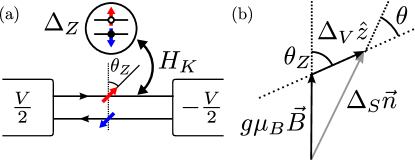
Figure 1: Setup considered in this paper (a) and construction of the effective QD Hamiltonian (b). A HLL is coupled to a QD described by a Kondo Hamiltonian $H_{K}$. A magnetic field $\vec{B}$ is applied to the QD, which is tilted with respect to the quantization axis $\hat{z}$ of the helical edge state (fixed by the helical edge) by an angle $\theta_{Z}$. The effective system Hamiltonian for the QD is the sum of a Zeeman term $g\mu_{B}\vec{B}\cdot\vec{S}$ and an induced part $\Delta_{V}S^{z}$ that corresponds to the spin-polarization of the HLL driven by a bias voltage $V$. The resulting effective field points along $\vec{n}$ with tilt-angle $\theta$ and has strength $\Delta_{S}$ (see text).

In this work, we discuss a setup in which a QD in the cotunneling regime is coupled to the QSH device, which acts as a spin polarized reservoir. In order to manipulate the spin on the QD, we assume that a magnetic field is applied to the QD, inducing a quantization axis that is not parallel with that of the QSH states that is determined by spin-orbit interaction. The resulting dynamics are described with a general master equation (GME) approach. From the GME we obtain the spin polarization of the QD and the transport signatures, including effects due to electron-electron interactions in the helical edge, which is crucial for these 1D channels. We discuss the possibilities to manipulate the state of the QD, and the signatures of these manipulations in the transport properties.

Model.– We consider a Zeeman split QD in the Coulomb blockade regime coupled to a HLL, as illustrated in Fig. 1(a). The Hamiltonian is given by (we set $\hbar=e=1$)

$$H=H_{\mathrm{HLL}}+H_{Z}+H_{K}.$$ (1)

The HLL is described by the Hamiltonian Wu2006

$$H_{\mathrm{HLL}} =v_{F}\int\mathrm{d}\xi\,:\sum_{\eta=\pm}\Psi_{\eta}^{\dagger}(-i\eta\partial_{\xi})\Psi_{\eta}(\xi):$$ (2)

$$\quad+\frac{\lambda}{2}\int\mathrm{d}\xi\,:\Big{(}\sum_{\eta=\pm}\Psi_{\eta}^{\dagger}(\xi)\Psi_{\eta}(\xi)\Big{)}^{2}:,$$

where $v_{F}$ is the Fermi velocity, $\Psi^{(\dagger)}_{\eta}$ are electron operators on the edge in branch $\eta=\pm$ corresponding to right and left movers, which are spin polarized parallel or antiparallel to the spin quantization axis $\hat{z}$ due to the helical nature of the HLL, and $\lambda$ is the interaction strength due to Coulomb repulsion in the helical edge. The QSH device is connected to leads and a bias $V$ is applied. As the electrons have a definite propagation direction correlated with spin, this induces a spin bias. The bias can be gauged into the lead operators Peca2003 .

In the cotunnelling regime, a single-level QD coupled to a HLL can be described by the Kondo Hamiltonian Hewson1993

$$H_{K}=J\big{(}J^{+}S^{-}+J^{-}S^{+}+2J^{z}S^{z}\big{)},$$ (3)

where $J$ is the Kondo coupling strength. The spin operators are defined by $J^{\tau}=\tfrac{1}{2}\sum_{\mu,\nu}\Psi_{\nu}^{\dagger}(0)\sigma^{\tau}_{\nu,\mu}\Psi_{\mu}(0)$ and $S^{\tau}=\tfrac{1}{2}\sum_{\mu,\nu}d_{\nu}^{\dagger}\sigma^{\tau}_{\nu,\mu}d_{\mu}$, where $\sigma^{\tau}$, $\tau=x,y,z$, are the Pauli matrices and where $d^{(\dagger)}_{\sigma}$ correspond to electrons with spin projection $\sigma$ on the QD with respect to $\hat{z}$. The ladder-operators are defined as $J^{\pm}=J^{x}\pm iJ^{y}$ and $S^{\pm}=S^{x}\pm iS^{y}$.

We allow for a general direction of the magnetic field $\vec{B}$ on the QD, and the Zeeman term obtains its standard form,

$$H_{Z}=g\mu_{B}\vec{B}\cdot\vec{S},$$ (4)

where $g$ is the $g$-factor, $\mu_{B}$ is the Bohr magneton, and $\Delta_{Z}=g\mu_{B}|\vec{B}|$ the resulting Zeeman splitting Note1 .

Spin dynamics for QD.– We consider the dynamics of the QD spin in the weak coupling limit ($J\to 0$) and derive a generalized master equation (GME) Koller2010 ; Breuer2002 ; Blum1996 for the reduced density matrix $\rho\equiv\textrm{Tr}_{B}\rho_{\mathrm{tot}}$ of the QD, where the degrees of freedom of the bath (the HLL) are traced out. For convenience, we redefine the system, bath, and interaction Hamiltonian as $H_{S}\equiv H_{Z}+2J\langle{J^{z}}\rangle_{0}{S^{z}}$, $H_{B}\equiv H_{\mathrm{HLL}}$, and $H_{I}\equiv H_{K}-2J\langle{J^{z}}\rangle_{0}{S^{z}}=\sum_{k=\pm,z}A_{k}S^{k}$, where the nonvanishing expectation value of $H_{K}$ is absorbed into $H_{S}$ Note (2). Indeed, due to the finite bias $V$, we have $\langle{J^{z}}\rangle_{0}=V/(8\pi v_{F})$, where $\langle{\ldots}\rangle_{0}$ denotes expectation values for the uncoupled system ($H_{I}=0$). Here, we also define $A_{\pm}\equiv J{J^{\mp}}$ and $A_{z}\equiv 2J({J^{z}}-\langle{J^{z}}\rangle_{0})$. $H_{S}$ describes the interaction with the external magnetic field and an effective HLL-induced one ($\propto JV$), as illustrated in Fig. 1(b). The total effective field is in the plane spanned by the HLL spin-quantization axis and the external field.

The effective magnetic field felt by the QD can be parametrized using polar coordinates $\theta$ and $\phi$. Defining $\Delta_{V}\equiv{}2J\langle{J^{z}}\rangle_{0}$, the system Hamiltonian can be written as

$$H_{S}=\Delta_{S}{\vec{n}}\cdot\vec{S},$$ (5)

where $\Delta_{S}=(\Delta_{V}^{2}+\Delta_{Z}^{2}+2\Delta_{V}\Delta_{Z}\cos\theta_{Z})^{1/2}$ and ${\vec{n}}=(\sin\theta\cos\phi,\sin\theta\sin\phi,\cos\theta)^{\rm T}$ is the direction of the effective magnetic field. The polar angle for this effective field is defined as $\theta\equiv\arccos[(\Delta_{Z}\cos\theta_{Z}+\Delta_{V})/\Delta_{S}]$, where $\theta_{Z}$ is the angle between $\vec{B}$ and lead quantization axis $\hat{z}$.

This Hamiltonian can be diagonalized by a unitary transformation $UH_{S}U^{\dagger}=\Delta_{S}{S^{\prime}}^{z}$ where ${S^{\prime}}^{z}$ is the spin along ${\vec{n}}$. This transformation corresponds to a rotation from the $\vec{S}$-operators to ${\vec{S}}^{\prime}$ -operators defined by $S^{i}=\sum_{ij}\mathscr{D}(U)_{ij}{{S^{\prime}}^{j}}$ where $i,j=z,+,-$ and

$$\mathscr{D}(U)=\begin{pmatrix}\cos\theta&-\tfrac{z_{\gamma}}{2}\sin\theta&-\tfrac{z_{\gamma}^{*}}{2}\sin\theta\\ z_{\phi}\sin\theta&z_{\phi}z_{\gamma}\cos^{2}\frac{\theta}{2}&-z_{\gamma}^{*}z_{\phi}\sin^{2}\frac{\theta}{2}\\ z_{\phi}^{*}\sin\theta&-z_{\gamma}z_{\phi}^{*}\sin^{2}\frac{\theta}{2}&z_{\gamma}^{*}z_{\phi}^{*}\cos^{2}\frac{\theta}{2}\end{pmatrix}.$$ (6)

Here, $z_{\phi}\equiv e^{i\phi}$ and $z_{\gamma}\equiv e^{i\gamma}$. As $H_{S}$ is invariant under rotation around ${\vec{n}}$, a free parameter $\gamma$ remains that will not influence the results in the lab-frame (unprimed-frame). For definiteness, we choose $\phi=\pi/2$ in the following so that ${\vec{n}}$ lies in the $y$-$z$-plane.

Generalized master equation.– Expanding up to second order in $H_{I}$ following standard steps Blum1996 , we arrive at the Redfield master equation,

$$\dot{\rho}^{I}(t)=-\int_{t_{0}}^{t}\mathrm{d}\tau\,\mathcal{K}^{I}(t,\tau)\{\rho^{I}(\tau)\}$$ (7a)

$$\mathcal{K}^{I}(t,\tau)\{\rho^{I}(\tau)\}=\sum_{k,l=\pm,z}e^{i\Delta_{S}(\sigma_{k}\tau+\sigma_{l}t)}\\ \times\left(\mathcal{G}_{k,l}(t-\tau)[{{S^{\prime}}^{k}},{S^{\prime}}^{l}\rho^{I}(\tau)]\right.\\ +\left.\mathcal{G}_{l,k}(\tau-t)[\rho^{I}(\tau){S^{\prime}}^{l},{S^{\prime}}^{k}]\right),$$ (7b)

where ${S^{k}}^{\prime}$ are the spin operators defined via Eq. (6), $\sigma_{\pm}=\pm 1$, $\sigma_{z}=0$ and $\mathcal{G}_{k,l}(\tau)\equiv\sum_{\alpha=\pm,z}c_{\alpha,k}c_{\bar{\alpha},l}G_{\alpha,\bar{\alpha}}(\tau)$, $G_{\alpha,\bar{\alpha}}(\tau)\equiv\langle A_{\alpha}(\tau)A_{\bar{\alpha}}(0)\rangle$, and $c_{k,l}\equiv(\mathscr{D}(U))_{k,l}$. The bar denotes interchange of $+$ and $-$, with $\bar{z}=z$. Assuming fast decaying bath correlation functions, the Markov approximation $\rho(t)\approx\rho(\tau)$ can be used. The terms for which $\sigma_{k}+\sigma_{l}\neq 0$ have a coefficient whose phase oscillates with $\Delta_{S}t$ whereas the relaxation time is proportional to $\gamma_{R}^{-1}$ where $\gamma_{R}=(J^{2}/v_{F}^{2}\beta)$ with $\beta=1/k_{B}T$ (see Eqs. (9)). For $\gamma_{R}\ll\Delta_{S}$, those terms can be neglected. Therefore, in the regime $\gamma_{R}\ll\Delta_{S},k_{B}T$, the GME is given in Lindblad form

$$\dot{\rho}^{I}(t) =-i[H_{\mathrm{LS}},\rho^{I}(t)]+\mathcal{D}(\rho^{I}(t))$$ (8a)

$$\mathcal{D}(\rho^{I}(t)) =\sum_{k,l=\pm,z}\mathcal{F}_{\bar{k},k}(-\Delta_{S}\sigma_{k})$$

$$\times\Big{(}{{S^{\prime}}^{k}\rho^{I}(t){{S^{\prime}}^{k}}^{\dagger}}-\frac{1}{2}\{{{S^{\prime}}^{k}}^{\dagger}{S^{\prime}}^{k},\rho^{I}(t)\}\Big{)},$$ (8b)

where $\mathcal{F}_{k,l}(\omega)\equiv\int_{-\infty}^{\infty}\mathrm{d}\tau\,e^{i\omega\tau}\mathcal{G}_{k,l}(\tau)=\sum_{\alpha=\pm,z}c_{\alpha,k}c_{\bar{\alpha},l}F_{\alpha,\bar{\alpha}}(\omega)$ are Fourier transforms of the bath correlation functions, and $H_{\mathrm{LS}}$ is a Lamb shift Hamiltonian. The latter does not influence the steady state, as it only leads to phase oscillations of the off-diagonal entries, which decay due to dephasing. The bath correlation functions can be found using a standard approach Giamarchi2007 ,

$$F_{zz}(\omega) =\gamma_{R}\frac{K}{2\pi}\frac{\omega\beta}{\sinh(\omega\beta/2)}e^{\frac{\omega\beta}{2}}$$ (9a)

$$F_{\pm,\mp}(\omega) =\gamma_{R}\frac{(2a)^{2K-2}\;e^{\frac{\beta}{2}(\omega\mp V)}}{\Gamma(2K)|\Gamma(1-K-i(\omega\mp V)\beta/2\pi)|^{2}}$$

$$\times\frac{K^{2}\pi}{\cosh((\omega\mp V)\beta)-\cos(2\pi K)},$$ (9b)

where $a\equiv K\pi\alpha/\beta v_{F}$ with $\alpha$ the short-distance cutoff and $K\equiv 1/\sqrt{(1+\lambda/\pi v_{F})}$ is the Luttinger liquid parameter. The resulting steady state is

$$\bar{\rho}=\frac{1}{\mathcal{F}_{+-}(\Delta_{S})+\mathcal{F}_{-+}(-\Delta_{S})}\begin{pmatrix}\mathcal{F}_{-+}(-\Delta_{S})&0\\ 0&\mathcal{F}_{+-}(\Delta_{S})\end{pmatrix}\,.$$ (10)

Note that $\bar{\rho}$ is diagonal only in the eigenbasis of $H_{S}$.

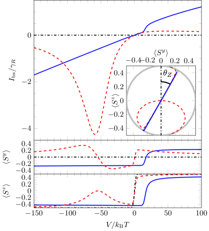
Figure 2: Backscattering current and QD spin-polarization (SP) in $y$ and $z$ direction for $J/v_{F}=0.1$, $\alpha/\beta v_{F}=10^{-3}$, $\theta_{Z}=\pi/6$, $\Delta_{Z}=15\leavevmode\nobreak\ k_{\mathrm{B}}T$ (blue solid), $\Delta_{Z}=0.5\leavevmode\nobreak\ k_{\mathrm{B}}T$ (red dashed) and $\Delta_{Z}=0$ (black dash dotted) as a function of the bias $V$ and for $K=1$ is shown. The inset shows the SP in the $z$-$y$-plane for the same bias range. For illustration, the Bloch sphere and the direction of the Zeeman field (with angle $\theta_{Z}$) are added in gray. When $|V|$ is comparable to $\Delta_{Z}$ the SP is along ${\vec{B}}$ whereas it is along ${\hat{z}}$ (the HLL quantization axis) when $|\Delta_{V}|$ is larger than $\Delta_{Z}$. The spin flip along the magnetic field direction and the peculiar change of the SP within the $z$-$y$-plane shows clear signatures in the backscattering current.

QD spin-polarization.– As the effective magnetic field along ${\vec{n}}$ is tilted with respect to the Zeeman field ${\vec{B}}$ and the lead quantization axis, the QD spin-polarization (SP) in $z$ and $y$ direction $\langle S^{z,y}\rangle={\rm Tr}[{\bar{\rho}}\,S^{z,y}]$ can deviate from both directions. In order to understand the effect of this tilt, the SP as a function of bias $V$ for several $\Delta_{Z}$ and a fixed tilt $\theta_{Z}$ is shown in the inset of Fig. 2. Three different regimes with respect to $\Delta_{Z}/\Delta_{V}$ can be distinguished. If $\Delta_{Z}$ vanishes, the system quantization axis ${\vec{n}}$, and hence the SP, is aligned or anti-aligned with the HLL quantization axis $(\theta=0,\pi)$ , depending on the sign of $V$ (dashed-dotted line in Fig. 2). If $\Delta_{Z}$ is finite, two further regimes can be distinguished. If $|\Delta_{V}|\ll\Delta_{Z}$ (full line in Fig. 2), the quantization axis of the QD is fixed to the direction of ${\vec{B}}$. For $|V|,k_{B}T\ll\Delta_{Z}$, the QD spin stays in the ground state. When $V\approx\Delta_{Z}$, the QD spin can flip and eventually will occupy mostly the excited state. When $-\Delta_{V}\mathop{\mathrm{sgn}}({\hat{z}}\cdot{\vec{B}})\approx\Delta_{Z}$ there is a strong bias dependence of $\theta$. The QD depolarizes ($\langle S^{z}\rangle=\langle S^{y}\rangle=0$) if $V\cos\theta=\Delta_{S}$, which can be reached for positive and negative bias voltages, as illustrated by the dashed line in Fig. 2. This feature is a direct consequence of the helical nature of the edge states.

HLL backscattering current.– The current correction due to the coupling to the QD in one of the $\eta$-branches of the HLL is given by $\hat{I}_{\eta}(t)=\dot{N}_{\eta}$, with

$$\dot{N}_{\eta}=i[H_{I}(t),N_{\eta}(t)]=i\eta(A_{+}(t)S^{+}(t)-A_{-}(t)S^{-}(t)),$$ (11)

where $N_{\eta}=\int d\xi\Psi^{\dagger}_{\eta}(\xi)\Psi_{\eta}(\xi)$. The steady state current can be obtained from $I_{\mathrm{bs}}=\lim_{t\rightarrow\infty}I_{-}(t)=\lim_{z\rightarrow 0^{-}}zI_{-}(z)$, where $I_{-}(z)$ is the Laplace transform of $\textrm{Tr}(\rho(t)\hat{I}_{-}(t))$. The current can now be obtained from the Born approximation for $\rho$. As the steady state density matrix is diagonal in the eigenbasis of $H_{S}$ we find for the backscattering current

$$I_{\mathrm{bs}}=\big{[}\cos^{4}\frac{\theta}{2}\big{(}F_{-+}(-\Delta_{S})\bar{\rho}_{\downarrow,\downarrow}-F_{+-}(\Delta_{S})\bar{\rho}_{\uparrow,\uparrow}\big{)}\\ +\sin^{4}\frac{\theta}{2}\big{(}F_{-+}(\Delta_{S})\bar{\rho}_{\uparrow,\uparrow}-F_{+-}(-\Delta_{S})\bar{\rho}_{\downarrow,\downarrow}\big{)}\\ +\frac{\sin^{2}\theta}{4}\big{(}F_{-+}(0)-F_{+-}(0)\big{)}\big{]}.$$ (12)

The rich backscattering transport characteristics of this system is shown in Figs. 2, 3 and 4. The backscattering current vanishes identically in the case $\theta=0,\pi$ (dashed-dotted line Fig. 2) which holds for ${\vec{B}}=0$ or if ${\vec{B}}$ is parallel or antiparallel to the HLL quantization axis (${\hat{z}}$), which can be seen explicitly from the first two lines in Eq. (12) noting that $\bar{\rho}_{\uparrow,\uparrow}/\bar{\rho}_{\downarrow,\downarrow}=F_{-+}(-\Delta_{S})/F_{+-}(\Delta_{S})$ in that case. This is consistent with the results given for the Kondo impurity in a HLL Tanaka2011 ; Vayrynen2014 , the isotropic Kondo impurity with Rashba interaction Eriksson2012 , and a QD in the Coulomb blockade regime connected to fully polarized antiparallel ferromagnetic leads Weymann2005a .

However, we find that the BSC is in general finite for non-zero angle $\theta$. We first consider the non-interacting case $K=1$. We start with the regime $|\Delta_{V}|\ll\Delta_{Z}$ where $\theta\approx\theta_{Z}$, displayed for the backscattering current in Fig. 2 (full line) as a function of bias voltage $V$ for a relatively small tilting angle $\theta_{Z}=\pi/6$ and in Fig. 3 for the BSC for various angles $\theta_{Z}$. The clear conductance peak at $V\approx\Delta_{Z}$ reflects the energy threshold to flip the spin $\downarrow\rightarrow\uparrow$ on the QD, releasing the bottleneck for backscattering processes. For a finite angle $\theta_{Z}$, the second line in Eq. (12) starts to contribute which leads to a finite dc-BSC. Increasing the angle $\theta_{Z}$ further results in a development of a mirror peak at $V\approx-\Delta_{Z}$ since now the QD spin has an appreciable overlap with both spin-directions in the HLL (see Fig. 3). In addition, a constant shift of the BSC originates from the third line of Eq. (12) which describes spin flip processes in the leads, but none on the QD, and is therefore independent of ${\bar{\rho}}$. Turning on HLL-interactions, an additional peak at zero bias, cut by temperature, starts to develop as well (see Fig. 4). However, the peaks at finite bias are still visible.

We now turn to the regime $-\Delta_{V}\mathop{\mathrm{sgn}}({\hat{z}}\cdot{\vec{B}})\approx\Delta_{Z}$, where $\theta$ strongly depends on the bias voltage $V$. The backscattering current in this regime is governed by a second peak as shown in Fig. 2 by the dashed line and reflects the sweep of the angle $\theta$ through $\pi/2$ as a function of $V$ whereas the fixed angle $\theta_{Z}=\pi/6$ is rather small. In accordance with the polarization plot in Fig. 2, the second current peak appears close to the depolarization of the QD ($\langle S_{z}\rangle=\langle S_{y}\rangle=0$) at finite negative bias voltage where $\theta\approx\pi/2$. At very large $|V|$, the current has to disappear as the effective quantization axis of the QD aligns ($V>0$) or anti-aligns ($V<0$) with the quantization axis of the HLL.

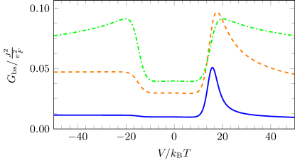
Figure 3: Differential conductance $G_{\rm bs}$ as a function of bias voltage $V$ for different tilt-angles: $\theta_{Z}=\pi/2$ (green dash dotted), $\theta_{Z}=\pi/3$ (orange dashed) and $\theta_{Z}=\pi/6$ (blue solid). $\Delta_{Z}=15\leavevmode\nobreak\ k_{\mathrm{B}}T$, $J/v_{F}=0.1$, $\alpha/\beta v_{F}=10^{-3}$ and $K=1$. $G_{\rm bs}$ shows a peak when $|V|\approx\Delta_{Z}$ with an asymmetry between $V>0$ and $V<0$ that vanishes when the Zeeman field is perpendicular to the lead quantization axis ($\theta_{Z}=\pi/2$).

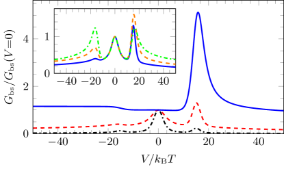
Figure 4: Renormalized differential conductance as a function of bias voltage $V$ for different HLL interaction strengths: $K=0.6$ (black dash dotted), $K=0.8$ (red dashed) and $K=1$ (blue solid). $\Delta_{Z}=15\leavevmode\nobreak\ k_{\mathrm{B}}T$, $J/v_{F}=0.1$, $\alpha/\beta v_{F}=10^{-3}$, and $\theta_{Z}=\pi/6$. The inset shows the renormalized differential conductance for the parameters from Fig. 3 with $K=0.8$.

Experimental feasibility.– Limiting the effect of ${\vec{B}}$ to the QD might be challenging in a real experiment, as e.g. a homogenous field influences also the helical edge. However, the orbital effect of the magnetic field Note (3) is not expected to destroy the helical property up to several Tesla in devices made from HgTe/CdTe QWs Tkachov2010 ; Tkachov2011 ; Scharf2012 ; Pikulin2014 ; Pikulin2014 . The desired Zeeman splitting $\Delta_{Z}$ is smaller than the voltage range we consider, which in turn is much smaller than the bulk band gap $2D$. Assuming that $g$-factors for QD and helical edge are similar, the gap opened in the helical edge by a spin-mixing field will not exceed the band gap. A gap will open at the Dirac point and mix the two spins there, but for momenta far away from that point the helical behavior is maintained by the spin-orbit interaction Note (4). For HgTe/CdTe QWs $D$ is approximately $10\,\mathrm{meV}$. For a short-distance cutoff $\alpha\approx v_{F}/D$, the figures shown here correspond to a temperature of $T\approx 116\,\mathrm{mK}$, which is experimentally feasible. For the parameters shown here the Kondo temperature $T_{K}\approx(D/k_{B})\exp(-\pi v_{F}/J)\ll T$. The backscattering current in Fig. 2 is then given in units of $16\leavevmode\nobreak\ \mathrm{pA}$. Similar arguments would apply to InAs/GaSb QWs. Novel proposed QSH materials with much larger bulk gaps Zhou2014 ; Zhang2014 ; Xu2013 ; Xiao2011 would allow for higher temperatures and hence energies, which would lead to larger transport signals.

In summary, we discuss the dynamics of a QD spin subject to a weak external Zeeman field coupled to a QSH edge state. The QD spin-polarization is determined by the sum of this external field and an effective field induced by the helical edge state spin bias. The transport signatures show a strong dependence on the relative orientation of magnetic field and quantization axis in the helical edge state. These effects enable electrical control of the QD spin, and the determination of the edge state spin direction. The knowledge of the spin direction, and its variation with energy Virtanen2012 ; Schmidt2012 , is crucial for understanding inelastic backscattering mechanisms and for spintronics applications.

BP and PR acknowledge financial support from the NTH school for contacts in nanosystems and the EU-FP7 project SE2ND. PV acknowledges financial support by the Academy of Finland. We acknowledge insightful discussions with W.A. Coish, E.M. Hankiewicz and A. Ström. PR acknowledges the hospitality of the Tokyo Institute of Technology, Japan, where part of the work has been carried out.

References

- (1)
- (2) M. Z. Hasan and C. L. Kane, Rev. Mod. Phys. 82, 3045 (2010).
- (3) X.-L. Qi and S.-C. Zhang, Rev. Mod. Phys. 83, 1057 (2011).
- (4) B. A. Bernevig, T. L. Hughes, and S.-C.Zhang, Science 314, 1757 (2006).
- (5) M. König, S. Wiedmann, C. Brüne, A. Roth, H. Buhmann, L. W. Molenkamp, X.-L. Qi, and S.-C. Zhang, Science 318, 766 (2007).
- (6) A. Roth, C. Brüne, H. Buhmann, L. W. Molenkamp, J. Maciejko, X.-L. Qi, and S.-C. Zhang, Science 325, 294 (2009).
- (7) C. Liu, T. L. Hughes, X.-L. Qi, K. Wang, and S.-C. Zhang, Phys. Rev. Lett. 100, 236601 (2008).
- (8) I. Knez, R.-R. Du, and G. Sullivan, Phys. Rev. Lett. 107, 136603 (2011).
- (9) C. Brüne, A. Roth, H. Buhmann, E. M. Hankiewicz, L. W. Molenkamp, J. Maciejko, X.-L. Qi, and S.-C. Zhang, Nat. Phys. 8, 485 (2012).
- (10) C. Wu, B. A. Bernevig, and S.-C. Zhang, Phys. Rev. Lett. 96, 106401 (2006).
- (11) Y. Tanaka, A. Furusaki, and K. A. Matveev, Phys. Rev. Lett. 106, 236402 (2011).
- (12) J. Maciejko, C. Liu, Y. Oreg, X.-L. Qi, C. Wu, and S.-C. Zhang, Phys. Rev. Lett. 102, 256803 (2009).
- (13) A. Schiller and K. Ingersent, Phys. Rev. B 51, 4676 (1995).
- (14) J. I. Väyrynen, M. Goldstein, Y. Gefen, and L. I. Glazman, arxiv:1406.6052.
- (15) E. Eriksson, A. Ström, G. Sharma, and H. Johannesson, Phys. Rev. B 86, 161103 (2012).
- (16) E. Eriksson, Phys. Rev. B 87, 235414 (2013).
- (17) A. Narayan, A. Hurley, and S. Sanvito, Appl. Phys. Lett. 103, 142407 (2013).
- (18) A. Hurley, A. Narayan, and S. Sanvito, Phys. Rev. B 87, 245410 (2013).
- (19) F. M. Hu, T. O. Wehling, J. E. Gubernatis, T. Frauenheim, and R. M. Nieminen, Phys. Rev. B 88, 045106 (2013).
- (20) F. Goth, D. J. Luitz, and F. F. Assaad, Phys. Rev. B 88, 075110 (2013).
- (21) A. M. Lunde and G. Platero, Phys. Rev. B 86, 035112 (2012).
- (22) A. Del Maestro, T. Hyart, and B. Rosenow, Phys. Rev. B 87, 65440 (2013).
- (23) M. Braun, J. König, and J. Martinek, Phys. Rev. B 7, 195345 (2004).
- (24) I. Weymann, J. König, J. Martinek, J. Barnaś, and G. Schön, Phys. Rev. B 72, 115334 (2005).
- (25) I. Weymann and J. Barnaś, Phys. Rev. B 73, 205309 (2006).
- (26) L. Y. Gorelik, S. I. Kulinich, R. I. Shekhter, M. Jonson, and V. M. Vinokur, Phys. Rev. Lett. 95, 116806 (2005).
- (27) D. Urban, M. Braun, and J. König, Phys. Rev. B 76, 125306 (2007).
- (28) C. S. Peça, L. Balents, and K. J. Wiese, Phys. Rev. B 68, 205423 (2003).
- (29) A. C. Hewson, The Kondo Problem to Heavy Fermions (Cambridge Univ. Press, Cambridge, 1993), 1st ed.
- (30) For definiteness, we assume in the paper. The case can be accounted for by reversing the sign of .
- (31) S. Koller, M. Grifoni, M. Leijnse, and M. R. Wegewijs, Phys. Rev. B 82, 235307 (2010).
- (32) H.-P. Breuer and F. Petruccione, The Theory of Open Quantum Systems (Oxford Univ. Press, Oxford, 2002).
- (33) K. Blum, Density Matrix Theory and Applications (Plenum Press, New York , 1996), 2nd ed.
- Note (2) Whether this redefinition is done or not does not affect the final GME to order .
- (35) T. Giamarchi, Quantum Physics in One Dimension (Oxford University Press, Oxford, 2003).
- (36) I. Weymann, J. Barnaś, J. König, J. Martinek, and G. Schön, Phys. Rev. B 72, 113301 (2005).
- Note (3) In Ref. Tkachov2010 it is shown that the orbital effect of a perpendicular magnetic field (along the spin axis of the helical edge state) is weak unless becomes much larger than one. Here, 37 nm is the bulk-penetration length of the edge state for HgTe-based QWs, and is the magnetic length. Using , gives the order of magnitude of 0.5 Tesla. This corresponds to a Zeeman splitting using Buttner2011 for HgTe based QWs.
- (38) B. Büttner, C. X. Liu, G. Tkachov, E. G. Novik, C. Brune, H. Buhmann, E. M. Hankiewicz, P. Recher, B. Trauzettel, S. C. Zhang, L. W. Molenkamp, Nat. Phys. 7, 418 (2011).
- (39) G. Tkachov and E. M. Hankiewicz, Phys. Rev. Lett. 104, 166803 (2010).
- (40) G. Tkachov and E. M. Hankiewicz, Phys. Rev. B 83, 155412 (2011).
- (41) B. Scharf, A. Matos-Abiague, and J. Fabian, Phys. Rev. B 86, 075418 (2012).
- (42) D. I. Pikulin, T. Hyart, S. Mi, J. Tworzydło, M. Wimmer, and C. W. J. Beenakker, Phys. Rev. B 89, 161403 (2014).
- Note (4) The admixture of the other spin component due to a Zeeman gap in the edge state is () with the Fermi wavenumber.
- (44) M. Zhou, W. Ming, Z. Liu, Z. Wang, Y. Yao, and F. Liu, (2014), arxiv:1401.3392 .
- (45) H. Zhang, Y. Xu, J. Wang, K. Chang, and S.-C. Zhang, Phys. Rev. Lett. 112, 216803 (2014).
- (46) Y. Xu, B. Yan, H.-J. Zhang, J. Wang, G. Xu, P. Tang, W. Duan, and S.-C. Zhang, Phys. Rev. Lett. 111, 136804 (2013).
- (47) D. Xiao, W. Zhu, Y. Ran, N. Nagaosa, and S. Okamoto, Nature Communications 2, 596 (2011).
- (48) P. Virtanen and P. Recher, Phys. Rev. B 85, 035310 (2012).
- (49) T. L. Schmidt, S. Rachel, F. von Oppen, and L. I. Glazman, Phys. Rev. Lett. 108, 156402 (2012).