Matrix Completion for the Independence Model
Abstract
We investigate the problem of completing partial matrices to rank-one matrices in the standard simplex . The motivation for studying this problem comes from statistics: A lack of eligible completion can provide a falsification test for partial observations to come from the independence model. For each pattern of specified entries, we give equations and inequalities which are satisfied if and only if an eligible completion exists. We also describe the set of valid completions, and we optimize over this set.
Key words: matrix completion; independence model; weighted graphs; tensor completion; real algebraic geometry; optimal completions.
AMS subject classifications: 15A83; 05C50; 14P10.
1 Introduction
The pattern of a partial matrix is the set of positions of specified entries in the partial matrix. A partial matrix is subordinate to if its pattern is . We are interested in the geometry of two semialgebraic sets: (1) the projection of rank-one matrices in to the entries in , and (2) the set of completions for a fixed partial matrix , as a subset of . Our exposition will be aimed at addressing the following two problems:
Problem 1.1.
Given , and , find defining equations and inequalities for the set of partial matrices subordinate to pattern that can be completed to a rank-one matrix in .
Problem 1.2.
Given a partial matrix and , characterize all rank-one matrices in whose projection to the entries in agree with .
Example 1.3.
Let , and . By our results in later sections, we can answer Problem 1.2 for the partial matrix on the left: there is a unique completion given by the matrix at right:
Perturbing any entry of the partial matrix by makes the set of completions empty, and perturbing any entry by introduces an infinite number of completions. We will also answer Problem 1.1 for this choice of , and : is completable if and only if .
The low-rank matrix completion is very well-studied: the three main directions have been convex relaxation of the rank constraints [5, 2, 3, 14], spectral matrix completion [7] and algebraic-combinatorial approach [4, 6, 10]. We make use of existing algebraic-combinatorial approaches in the latter three articles in our analysis. Our contribution is looking at how the two conditions – (1) nonnegativity and (2) summing to one – affect the rank-one completion problem. The perspective of the paper is a combinatorial and geometric rather than an algorithmic one, but we examine algorithms as they relate to the geometry.
The motivation for restricting to the simplex comes from statistics, and was suggested by Vishesh Karwa and Aleksandra Slavković. Let and be two discrete random variables with and states respectively. Their joint probabilities are recorded in the matrix: , where . For any such matrix , we have for all and . We say that random variables and are independent, if for all . This can be translated into the statement
Hence, the matrix of joint probabilities of two independent random variables has rank one, is nonnegative, and its entries sum to one. In other words, is a rank-one matrix in the standard simplex .
Our problems are of interest when probabilities are measurable only for certain pairs . Situations in which this might arise in applications are: a pair of compounds in a laboratory that only react when in certain states, a pair of alleles whose effects cancel each other out, etc. A complete answer to Problem 1.1 will allow us to reject a hypothesis of independence of the events and , based only on this collection of probabilities. For other problems about matrix completion coming from statistics see [8] and [15]. In the rest of the paper we will not consider the statistical context. Addressing questions like noise, the details of the falsification test, and experiments are left for a more statistical paper in the future.
Outline. In Section 2, we derive for given , and inequalities and equations which are fulfilled by the entries of a partial matrix subordinate to if and only if the partial matrix is completable to a rank-one matrix in . Our discussion starts with positive diagonal partial matrices in Section 2.1, continues with positive block partial matrices in Section 2.2 and positive general partial matrices in Section 2.3. Finally, Section 2.4 extends these results to nonnegative general partial matrices. The main result for positive partial matrices is described in Theorem 2.12 and for nonnegative partial matrices in Theorem 2.18. The Section 2 ends with an algorithm for checking completability of a partial matrix to a rank-one matrix in .
In Section 3, we describe the various completions for a given partial matrix. In Section 3.1, we show how to construct a completion for a positive partial matrix. In Section 3.2, we will use Lagrange multipliers to construct a rank-one completion in the standard simplex which maximizes or minimizes a certain function, e.g. the distance from the uniform distribution. In Section 3.3, we describe the set of completions when the partial matrix contains zeros.
In Section 4, we study generalization of our results to higher rank matrices and tensors in the standard simplex. In particular, in Theorem 4.1 we will derive a characterization of diagonal partial tensors which can be completed to rank-one tensors in the standard simplex, i.e. rank-one tensors whose entries are nonnegative and sum to one.
Partial tensors subordinate to a pattern which can be completed to a rank-one tensor in the standard simplex form a semialgebraic set, see Proposition 5.1. In Proposition 5.2, we study the algebraic boundary of this semialgebraic set.
Implementations of algorithms can be found on
| math.upenn.edu/zvihr/probCompletion.html |
2 Completability : Equations and Inequalities
In this section, we completely solve Problem 1.1 for all patterns . We begin by solving the problem for diagonal patterns, and then extrapolate to cases of increasing generality:
Diagonal Block General.
Initially, we will only consider positive partial matrices, and find its defining equations and inequalities. In Section 2.4, we will consider partial matrices with zero entries.
2.1 Diagonal Patterns
A diagonal partial matrix is an partial matrix (a point in ) subordinate to the diagonal pattern . In the case, this is trivially completable, indeed completed, if and only if the observed entry is one. For a matrix, there is more to consider.
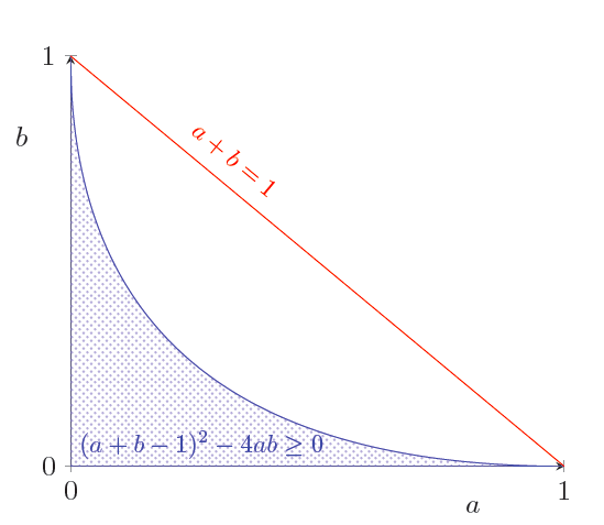
Example 2.1.
Let be the partial matrix given by: . In order for the matrix to be completed, both the rank one requirement and the summing to one must be addressed. First, for rank one, the off-diagonal entries are set to and , then the quantity is set equal to one. The equivalent quadratic equation is . In order for a real solution for to exist, the discriminant must be , i.e.
This inequality, along with the requirement that and both , is necessary and sufficient to guarantee that gives a completion in , see Figure 1.
For , we take advantage of the factorization of rank-one matrices as products of vectors to obtain the following more general result:
Theorem 2.2.
Let be an diagonal partial matrix given by , where , and for all . Then is completable if and only if , or equivalently, .
Proof.
Recall that a rank-one matrix can be factored as for . For this problem, consider all possible values of in , but do not restrict the values of to the simplex. Instead, let be formulated in terms of and the entries of the matrix. Explicitly, we have . An eligible completion will arise when . Here we assume and thus for all .
Let and compute the minimum of on the simplex. For this computation, consider as independent variables and .
Setting for all implies is constant for all . Since is in the simplex, we have equal to . The value of (i.e. the sum of ) at this point is . If this is , continuity of implies that a completion exists somewhere between our minimum and the boundary, because within an of the boundary of , we have
If this minimum value is , the function will not achieve anywhere in the simplex, so no completion is possible. ∎
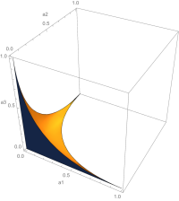
Remark 2.3.
The set of diagonal partial matrices that are completable to rank-one matrices in the standard simplex is shown in Figure 2.
2.2 Block Diagonal Patterns
We say that is a block of specified entries if the entries specified in rows and columns are exactly . A block partial matrix is a partial matrix subordinate to a pattern that is the union of blocks of specified entries and every row and column contains at least one specified entry. We begin with a corollary to Theorem 2.2.
Corollary 2.4.
Let be a partial matrix with a rank-one block of positively specified entries . Let be the partial matrix obtained from by contracting rows to one row, columns to one column and specifying
The completability of is equivalent to completability of .
Proof.
() Let be a completion of . Then one completion of is:
() Let be a
completion of , where
and . Since
form a rank-one matrix,
it has a rank-one factorization . Then one completion of is:
∎
The corollary implies that a rank-one block in the upper-left corner of a matrix can be replaced by the sum of its entries without changing the completability of the full matrix. The same logic applies to any rank-one block in the matrix, since row and column permutations do not affect rank or the value of the sum of entries. We then have this result for block partial matrices.
Corollary 2.5.
Let be a block partial matrix with rank-one blocks of positively specified entries. Let be a diagonal partial matrix with one diagonal entry for each block of specified entries of . Let a diagonal entry of be equal to the sum of entries in the corresponding block of specified entries of . Then completability of is equivalent to completability of .
2.3 General Partial Matrices
To discuss general partial matrices, we introduce graph notation used in the matrix completion literature, including for example [10].
Definition 2.6.
Let be a matrix in , and let and be vectors in and respectively. A bipartite graph can be associated to in the following way:
Graph Matrix White vertex -th row Black vertex -th column Edge -th entry Weight Sum of -th row, or Weight Sum of -th column, or Edge weight Value of entry
The bipartite graph associated to a partial matrix is the graph obtained by deleting the edges corresponding to unobserved entries, and omitting vertex weights. If we want to talk about the corresponding unweighted graph, then we say the bipartite graph associated to a pattern .
Example 2.7.
On the left is a partial matrix and on the right is the corresponding bipartite graph.
In this formulation, the question of completability is equivalent to the existence of a vertex labeling so that the black vertex weights and white vertex weights each sum to one, and the edge weights satisfy . The edge set of the bipartite graph associated to a diagonal partial matrix forms a perfect matching of . The bipartite graph associated to a block partial matrix is the union of disjoint complete bipartite graphs. We now consider more general partial matrices and bipartite graphs. For this we introduce a definition and a lemma paraphrased from [4, Section 6]:
Definition 2.8 ([4]).
Let be a pattern with corresponding bipartite graph . Call a cycle in if is a cycle in .
Let be a partial matrix with pattern , and let be the entry in corresponding to the edge in . The partial matrix will be called singular with respect to a cycle in if
| (2.1) |
Lemma 2.9 ([4], Lemma 6.2).
Let be a partial matrix subordinate to a pattern with all specified entries positive. Then the minimal rank over all completions of is one if and only if is singular with respect to all cycles in .
In Lemma 2.9, a completion means any completion and not necessarily a rank-one completion in the standard simplex as in the rest of the paper. Lemma 2.9 gives a necessary condition for a rank-one completion to exist.
The algorithm for completing the uniquely completable entries in a rank-one completion is given implicitly in the proof of [4, Lemma 6.2] and stated explicitly in [6, Formula 6], [10, Theorem 34] and [9, Theorem 2.6]. We describe the algorithm as it is written in the proof of [4, Lemma 6.2]:
Algorithm 2.10.
Let be an unspecified entry. Let be a cycle in which was not a cycle in . One of the edges in this cycle is , say . Let and . Then, set
| (2.2) |
The following corollary in [6, 10, 9] establishes which entries of a partial matrix are uniquely reconstructible by cycles if the partial matrix does not contain zeros:
Corollary 2.11 ([6], Corollary 6, [10], Theorem 34, [9], Theorem 2.4).
Let be a partial matrix subordinate to a pattern with all specified entries non-zero. The set of uniquely reconstructible entries of is exactly the set with in the transitive closure of . In particular, all of is reconstructible if and only if is connected.
The transitive closure of a bipartite graph is the graph that is obtained from by replacing each connected component by a complete bipartite graph on the vertices that belong to the connected component. Suppose that a partial matrix has all positive entries and is singular with respect to cycles in , the completability of is equivalent to the completability of together with its uniquely reconstructible entries. By Corollary 2.11, this is a partial matrix that consists of non-zero blocks.
Theorem 2.12.
Let be the set of positive partial matrices subordinate to the pattern that can be completed to a rank-one matrix in . Define entries corresponding to the edges in the transitive closure using Formula (2.2). Let be the number of connected components of that contain at least one edge, let be the -th block of , and let be the sum of the weights in .
-
1.
If , the defining constraints for are:
-
(a)
the ideal generated by relations (2.1) corresponding to cycles of , and ; and
-
(b)
the inequalities for all .
-
(a)
-
2.
Otherwise the defining constraints for are:
-
(a)
the ideal generated by relations (2.1) corresponding to cycles of ; and
-
(b)
the inequalities for all , and .
-
(a)
Proof.
In both parts the ideal of relations corresponding to cycles of ensures that the conditions of Lemma 2.9 are satisfied. By Corollary 2.11 and Corollary 2.4, we can reduce to the diagonal partial matrix case with possibly some empty rows and columns. A completion of the matrix with empty rows and columns removed gives a completion of the original matrix by setting all the entries in the empty rows and columns equal to zero. A completion of the original matrix gives a completion of the matrix with empty rows and columns removed with the sum of entries . By the continuity argument as in the proof of Theorem 2.2, this matrix has a desired completion. Finally we apply Theorem 2.2. ∎
Note that these defining equations and inequalities include rational functions and algebraic functions like square root. The Tarski-Seidenberg Theorem ensures that these can be converted into polynomial equations and inequalities; we will explore this in more detail in Section 5.
Example 2.13.
The partial matrices of pattern with all observed entries positive has a completion if and only if
This is equivalent to the conditions
By clearing the denominators, we get polynomial inequalities in the observed entries whose solutions are all completable partial matrices of pattern .
2.4 Boundary of the Set of Completable Matrices
As promised, we discuss the set of partial matrices which have some specified entries equal to zero. Fix a pattern and let be the subset of entries set to zero. Specifically, for , and for .
Proposition 2.14.
A diagonal partial matrix is completable to a rank-one matrix in if and only if for and .
Proof.
Necessity of the conditions follows by the Cauchy-Schwarz inequality; sufficiency is given case by case: For , all rows and columns containing zeros may be set to zero, and the remaining submatrix can be completed by Theorem 2.2. For , without loss of generality take . Set
will be a completion of the matrix. For , simply set some off-diagonal entry to one and all other entries to zero. ∎
The strategy used in this proof is our general approach to dealing with zeros. We reduce to a smaller positive submatrix by removing some rows and columns. We use the same approach to pass to general submatrices; first we cite another definition from [4].
Definition 2.15 ([4]).
We say that is a 3-line in if is of the form
where and . In other words, is a line consisting of three edges in . The matrix will be called singular with respect to a 3-line in if either or (or both). This is equivalent to the zero row or column property in [6] that states that if any entry of a rank-one matrix is zero, then either every other entry of in the same row is zero or every other entry in the same column is zero.
Lemma 2.16 ([6], Lemma 1).
If a partial matrix has a rank-one completion, then it is singular with respect to 3-lines or equivalently it has the zero row or column property.
Definition 2.17.
Let , and . Let be the subset of such that:
-
1.
for , if and only if or , and
-
2.
for the pattern induced by restricting to the conditions of Theorem 2.12 are satisfied.
Theorem 2.18.
Let be a pattern of specified entries. Then the set of partial matrices subordinate to pattern which can be completed to a rank-one matrix in is given by
Proof.
Example 2.19.
Let be a pattern as a subset of matrices. In Table 1, the entry in row and column is a letter referring to a defining equation or inequality (up to change of index).
For instance, the entry in row , column corresponds to setting no rows equal to zero and the second column equal to zero. The resulting set is cut out by:
The geometry gives rise to an algorithm for deciding completability:
Algorithm 2.20 (Decide completability for a partial matrix ).
-
1.
Translate into the corresponding bipartite graph including edge weights.
-
2.
Check whether is singular with respect to 3-lines and cycles. If a 3-line or a cycle fails, return “NO”.
-
3.
Execute rank-one completion using 3-lines. Remove vertices that are connected to every vertex in a partite set with weight zero.
-
4.
Execute rank-one completion using cycles. Let the graph obtained after this step have connected components .
-
5.
If and the edge weights add up to one, return “YES”. Else, return “NO”.
-
6.
Let where is the sum of the entries in . If , return “NO”. Else, return “YES”.
Remark 2.21.
This algorithm runs in polynomial time in . Feasibility check and completion by cycles for each entry of the matrix runs in linear time in the number of observed entries by [9, Algorithm 2]. Feasibility check and completion by 3-lines is , where is the number of observed entries: For each zero one checks whether there is a non-zero entry in the column and in the row containing it. If there is a non-zero entry in both, then the partial matrix is not singular with respect to 3-lines. If there is a non-zero entry in the row, then complete all the entries in the column to zero (and vice-versa). If neither row nor column contains non-zero entries, then do nothing.
3 The Set of Completions
Throughout Section 2, we needed to prove the existence of a rank-one completion in the standard simplex for a partial matrix. Now, we assume existence of such a completion, and seek to describe all completions. For the beginning of this discussion, we assume no coordinates of are zero. This case will be addressed in Section 3.3.
3.1 Completions for Positive Partial Matrices
Theorem 3.1.
Let be a completable partial matrix with positive entries, subordinate to pattern . Let be the block-diagonal partial matrix obtained by completing with Formula (2.2). Let be the number of blocks in . Let be the sum of the weights in each block.
-
1.
if , then there is a unique completion;
-
2.
if and one component is an isolated vertex, there is a unique completion;
-
3.
if and both components contain edges, there are two completions;
-
4.
if , then there is an -dimensional basic semialgebraic set of completions.
Proof.
The unique completion for . The logic follows from the proof of Theorem 2.2; the diagonal matrix is given by . Since the diagonal version of the matrix has a unique solution there, the completion of the original partial matrix is uniquely determined by it.
The completion for with an isolated vertex. Complete the non-empty block, and let the block sum be . Because one row or column is left, simply add a copy of the first row or column and scale it until the sum is one.
The two completions for with two non-empty components. Complete the two non-empty blocks. If , then the factorization below
fails to keep the first factor in the simplex. Letting this vector vary as the second factor moves to the edges of the simplex, the sum of the coordinates is strictly increasing. Using the formula in Proposition 3.3, we can find the two points where the first factor lies in the simplex.
The -dimensional set of completions for . We start as in the case at the parametrization
Again the parametrization which matches our given values fails to have a first factor in the simplex. As we move to the boundary of the simplex along any direction, the sum in the first factor will hit . Therefore, the set of completions is parametrized by the sphere . ∎
In the diagonal partial matrix case we will explicitly describe the semialgebraic set. One can use results in Section 2 to derive semialgebraic descriptions in other cases. Let and define . Let us parametrize a vector by
where . Then
Proposition 3.2.
The semialgebraic set of completions of a diagonal partial matrix is given by and (after clearing denominators).
Any path from the local minimum to the boundary of the simplex will strike at least one solution. If any completion is acceptable, we can designate a simple path and find its points of intersection with the semialgebraic set of completions.
Proposition 3.3.
Let , such that and . Then, a completion of is given by:
where is one of the solutions to the following quadratic equation:
| (3.1) |
both of which lie in the interval .
Proof.
The trajectory traced for values of , is a line segment on the simplex. Setting the sum of the coordinates of equal to one and clearing denominators gives the quadratic equation above. Since it passes through the local minimum, continuity implies existence of two solutions in the desired interval. ∎
Example 3.4.
Consider the matrix . To obtain a completion, one may solve the quadratic equation (3.1), which after scaling turns into
giving solutions , or . Using the latter value, we obtain the matrix completion:
3.2 Optimization on a Completion Set
When the graph has connected components which contain at least an edge and , there is an -dimensional set of completions. For example, consider a diagonal partial matrix with each observed entry equal to the same constant . In Figure 3, each curve represents values of that parametrize a completion of the partial matrix with on the diagonal, for various values of . Here is projected onto the first two coordinates.
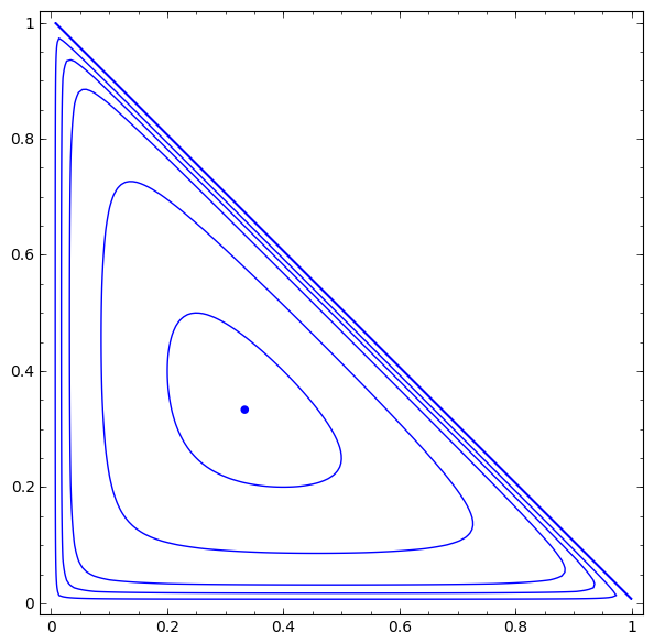
If we have infinitely many completions, one way to find a desired completion is to minimize or maximize a distance measure from a fixed matrix in the standard simplex. We will explain how to use Lagrange multipliers to solve this optimization problem if is the Euclidean distance from the uniform distribution.
By the method of Lagrange multipliers, an element in this semialgebraic set is a critical point for a distance function if and only if the gradient of is a constant multiple of the vector of partial derivatives . To compute all the critical points of the function on the variety given by , we need to solve the system of rational equations given by and all the minors of the matrix
Finally we need to check for all real solutions which satisfy which one minimizes the distance .
Example 3.5.
Consider the matrix . Find a completion that minimizes the Euclidean distance from the uniform distribution:
We use the Euclidean distance, but this method can be used for any distance measure.
We construct the Lagrange matrix
and find the critical points of on the variety by solving the system of rational equations . We use maple to construct and to solve the system of equations. This system has solutions, out of which ten are real and four are feasible, i.e. they satisfy . The minimum is achieved at
The Euclidean distance from the uniform distribution is .
3.3 Completions for Partial Matrices with Zeros
Now we consider those partial matrices that have zeros among their entries.
Definition 3.6.
Let be a partial matrix subordinate to a pattern . Define to be the set of completions of such that the rows in and the columns in are set to zero.
This is only well-defined where are precisely the zero-labeled elements of .
Proposition 3.7.
Let be a pattern, and let be the subset of zero entries. Let be the set of vertex covers of so that no vertex is adjacent to an edge of . Then the set of completions for subordinate to is given by:
Proof.
All of the zero entries must be in a zero row or a zero column - for this reason, we need a vertex cover. No nonzero entry may be in a zero row or zero column. This is why no vertex may be adjacent to an edge of . The result follows from there. ∎
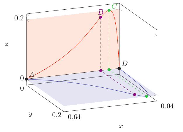
Example 3.8 (Two components in solution set).
Figure 4 describes the set of completions for the matrix , by plotting all possible values of ; the indicated matrix coordinates give an isomorphism between the two pictured curves and all completions of . Each curve comes from a minimal vertex cover of the set of zero entries: the red curve takes column 3, and the blue curve takes row 3. The components corresponding to two minimal vertex covers intersect at points corresponding to their union.
From left to right, we have the following matrices moving along the red curve:
The matrix at point represents the point at which the bottom row has largest possible row sum. The matrix at point has the largest possible value for . Following along the blue curve, we would pass through and .
4 Generalizations : Rank-1 Tensors and Rank-2 Matrices
In this section, we will consider the more general setting of tensors. The reader may consult [12] for an introduction on tensors and tensor rank. The notions of partial tensor, completion and pattern are analogous to the matrix case. Readers who are interested only in matrices can read other sections independently of this section.
4.1 Diagonal Partial Tensors
Theorem 2.2 for diagonal partial matrices generalizes nicely to diagonal partial tensors:
Theorem 4.1.
Suppose we are given an order- partial tensor with nonnegative observed entries along the diagonal, i. e. we have for , and all other entries unobserved. Then is completable if and only if
Proof.
The proof is analogous to the proof of Theorem 2.2, with a few adjustments to deal with the multiple parametrizing vectors. The tensor can be factored as , where each . The relations imply that the coordinates of can be expressed as functions on the product of simplices . Define by:
Since every variable appears in the denominator of some term, the function approaches infinity at the boundary of the product of simplices. A candidate vector will be available if and only if the minimum value of on the product of simplices is less than or equal to one. To find the minimum, compute partial derivatives; as in the proof of Theorem 2.2, we let for each .
Setting the partial derivatives to zero gives us the following:
Let be the value on both sides of this equation. Picking two values of , w.l.o.g., and , this designation means:
Applying to all indices, we have for all . Since for all , implying that every , and
for some constant . Since the sum , the value of . Plugging in these values of , we obtain
Since is at its minimum here, the value must be less than or equal to one for a solution to exist, proving the theorem. ∎
4.2 General Partial Tensors
Generalization to higher-order tensors brings several challenges. Theorem 4.1 gives a partial result characterizing diagonal tensors. However, the nice bipartite graph structure we had for matrices becomes -partite hypergraphs with -hyperedges; notions like connectivity will need to be modified. So, while any rank-one matrix completability problem was reducible to a diagonal case, the tensor case does not seem to be reducible in the same way. We record here the results for the smallest case distinct from matrices:
Example 4.2 ( Tensors).
The variety of rank-one tensors whose entries sum to one is -dimensional. For this example, we look only at algebraically independent sets of entries, so as to extract the semialgebraic constraints. We use the octahedral symmetry group of the cube to restrict to combinatorially distinct examples.
-
1.
(Size ) Any singleton, e.g. . The only condition is .
-
2.
(Size ) Three orbits of pairs:
-
(a)
: .
-
(b)
: .
-
(c)
: .
-
(a)
-
3.
(Size ) Three orbits of triples:
-
(a)
: .
-
(b)
: .
-
(c)
: The tensor is completable if and only if the equation
has a root in the interval .
-
(a)
In this example, five of the seven cases are equivalent to partial matrix problems. Only 2(c) and 3(c) use techniques that do not fall immediately out of the matrix case; still, the approach is analogous.
4.3 Low-Rank Matrices
One natural direction to generalize these results would be to fix rank , and find conditions for a matrix to be rank or nonnegative rank and have nonnegative entries that sum to one. One obvious consequence of our results is that any matrix completable to rank one is trivially completable as a higher-rank matrix. It is harder to provide tighter conditions, however, even in the smallest examples.
Example 4.3 ().
There are two polynomials constraining the entries of a rank matrix in the standard simplex: the determinant must be zero, and the sum of the entries must be one. The variety of matrices with these properties has dimension .
We take two combinatorially distinct partial matrices with seven entries. To find completions, we substitute and for the missing entries, where :
Since the sum is now fixed at one, we only need to check that there is a value of in so that the determinant is zero. In the first case the determinant gives a linear equation in , while in the second case the determinant is a quadratic; the solutions to each are:
Substituting the values in each matrix yields a completion for A, but since the discriminant of B is negative, no completion is possible.
From the statistics viewpoint, it would be more interesting to study completability to matrices in the standard simplex of nonnegative rank at most , because the -th mixture model of two discrete random variables is the semialgebraic set of matrices of nonnegative rank at most . If a nonnegative matrix has rank or , then its nonnegative rank is equal to its rank. Hence, in Example 4.3, we simultaneously address the question of completing a partial matrix to a matrix in the standard simplex of nonnegative rank .
If , then matrices of nonnegative rank at most form a complicated semialgebraic set. For , a semialgebraic description of this set is given in [11, Theorem 3.1]. Partial matrices that are completable to matrices in the standard simplex of nonnegative rank at most are coordinate projections of this semialgebraic set.
5 Semialgebraic Description
A reader interested only in matrices can replace everywhere in this section “tensor” by “matrix”.
Proposition 5.1.
Partial tensors subordinate to a pattern that are completable to rank-one tensors in the standard simplex form a semialgebraic set.
Proof.
The independence model is a semialgebraic set defined by -minors of all flattenings, nonnegativity constraints and entries summing to one. The statement of the proposition follows by the Tarski-Seidenberg theorem. ∎
The goal of this section is to find a semialgebraic description of this semialgebraic set, see [1] for an introduction to real algebraic geometry. The difference from characterizations in Theorems 2.2 and 2.12 is that we aim to derive a description without square roots. For partial matrices with diagonal entries, a semialgebraic description is given in Example 2.1 and its derivation from the inequality containing square roots is explained in Remark 2.3.
We will characterize the semialgebraic set of diagonal partial tensors which can be completed to rank-one tensors in the standard simplex. This is the positive part of the unit ball in the space.
Proposition 5.2.
There exists a unique irreducible polynomial of degree with constant term one that vanishes on the boundary of the set of diagonal partial tensors which can be completed to rank-one tensors in the standard simplex. The semialgebraic description takes the form , coordinates plus additional inequalities that separate our set from other chambers in the region defined by .
The proof of Proposition 5.2 was suggested to us by Bernd Sturmfels. For analogous proof idea, see [13, Lemma 2.1].
Proof.
Denote the diagonal entries of the partial tensor by . We will show that the defining polynomial of the -unit ball can be written as
| (5.1) |
We want to eliminate from the ideal
First replace by in the equation . We consider the field of rational functions . Solving the first equations is equivalent to adjoining the -th roots of for to the base field. This gives an extension of degree over . The group of all automorphisms of that leave fixed is . The product over all elements in the orbit of gives (5.1), and thus lies in the base field . Every factor in the product (5.1) is integral over , hence the product (5.1) is a degree polynomial in . No subproduct is left invariant under the automorphism group, so (5.1) is irreducible. ∎
ACKNOWLEDGEMENTS
We thank Bernd Sturmfels for introducing this problem to us, suggesting the proof of Proposition 5.2 and providing detailed feedback on the first draft of this article; Vishesh Karwa and Aleksandra Slavković for suggesting the problem; Thomas Kahle for sharing his ideas on the project; Mario Kummer for correcting a mistake in the proof of Proposition 5.2; Louis Theran for helping us with the complexity of algorithms. We also thank the anonymous referees for correcting several mistakes and aiding in the exposition. This collaboration was initiated while both authors were guests of the Max-Planck Institute for Mathematics, and was continued at the as2014 conference at Illinois Institute of Technology.
References
- [1] Saugata Basu, Richard Pollack, and Marie-Françoise Roy. Algorithms in real algebraic geometry, volume 10 of Algorithms and Computation in Mathematics. Springer-Verlag, Berlin, second edition, 2006.
- [2] Emmanuel J. Candès and Benjamin Recht. Exact matrix completion via convex optimization. Found. Comput. Math., 9(6):717–772, 2009.
- [3] Emmanuel J. Candès and Terence Tao. The power of convex relaxation: Near-optimal matrix completion. IEEE Trans. Inf. Theor., 56(5):2053–2080, 2010.
- [4] Nir Cohen, Charles R. Johnson, Leiba Rodman, and Hugo J. Woerdeman. Ranks of completions of partial matrices. In The Gohberg anniversary collection, Vol. I (Calgary, AB, 1988), volume 40 of Oper. Theory Adv. Appl., pages 165–185. Birkhäuser, Basel, 1989.
- [5] Maryam Fazel, Haitham Hindi, and Stephen P. Boyd. A rank minimization heuristic with application to minimum order system approximation. In Proceedings of the 2001 American Control Conference, volume 6, pages 4734–4739. IEEE, 2001.
- [6] Don Hadwin, K. J. Harrison, and Josephine A. Ward. Rank-one completions of partial matrices and completely rank-nonincreasing linear functionals. Proc. Amer. Math. Soc., 134(8):2169–2178, 2006.
- [7] Raghunandan H. Keshavan, Andrea Montanari, and Sewoong Oh. Matrix completion from a few entries. IEEE Trans. Inf. Theor., 56(6):2980–2998, 2010.
- [8] Gary King. A Solution to the Ecological Inference Problem: Reconstructing Individual Behavior from Aggregate Data. Princeton University Press, Princeton, 1997.
- [9] Franz J. Király and Louis Theran. Error-minimizing estimates and universal entry-wise error bounds for low-rank matrix completion. In C.J.C. Burges, L. Bottou, M. Welling, Z. Ghahramani, and K.Q. Weinberger, editors, Advances in Neural Information Processing Systems 26, pages 2364–2372. Curran Associates, Inc., 2013.
- [10] Franz J Király, Louis Theran, and Ryota Tomioka. The algebraic combinatorial approach for low-rank matrix completion. J. Mach. Learn. Res., 16:1391–1436, 2015.
- [11] Kaie Kubjas, Elina Robeva, and Bernd Sturmfels. Fixed points of the EM algorithm and nonnegative rank boundaries. Ann. Statist., 43(1):422–461, 2015.
- [12] Joseph M. Landsberg. Tensors: geometry and applications, volume 128 of Graduate Studies in Mathematics. American Mathematical Society, Providence, RI, 2012.
- [13] Jiawang Nie, Pablo A. Parrilo, and Bernd Sturmfels. Semidefinite representation of the -ellipse. In Alicia Dickenstein, Frank-Olaf Schreyer, and Andrew J. Sommese, editors, Algorithms in Algebraic Geometry, volume 146 of The IMA Volumes in Mathematics and its Applications, pages 117–132. Springer, New York, 2008.
- [14] Benjamin Recht. A simpler approach to matrix completion. J. Mach. Learn. Res., 12:3413–3430, 2011.
- [15] Bernd Sturmfels and Caroline Uhler. Multivariate gaussians, semidefinite matrix completion, and convex algebraic geometry. Ann. Inst. Stat. Math., 62(4):603–638, 2010.