Log-normal distribution based EMOS models for probabilistic wind speed forecasting

Abstract

Ensembles of forecasts are obtained from multiple runs of numerical weather forecasting models with different initial conditions and typically employed to account for forecast uncertainties. However, biases and dispersion errors often occur in forecast ensembles, they are usually under-dispersive and uncalibrated and require statistical post-processing. We present an Ensemble Model Output Statistics (EMOS) method for calibration of wind speed forecasts based on the log-normal (LN) distribution, and we also show a regime-switching extension of the model which combines the previously studied truncated normal (TN) distribution with the LN.

Both presented models are applied to wind speed forecasts of the eight-member University of Washington mesoscale ensemble, of the fifty-member ECMWF ensemble and of the eleven-member ALADIN-HUNEPS ensemble of the Hungarian Meteorological Service, and their predictive performances are compared to those of the TN and general extreme value (GEV) distribution based EMOS methods and to the TN-GEV mixture model. The results indicate improved calibration of probabilistic and accuracy of point forecasts in comparison to the raw ensemble and to climatological forecasts. Further, the TN-LN mixture model outperforms the traditional TN method and its predictive performance is able to keep up with the models utilizing the GEV distribution without assigning mass to negative values.

Key words: Continuous ranked probability score, ensemble calibration, ensemble model output statistics, log-normal distribution.

1 Introduction

Accurate and reliable forecasting of wind speed is of importance in various field of economy, e.g., agriculture, transportation, energy production. Forecasts are usually based on current observational data and mathematical models describing the dynamical and physical behaviour of the atmosphere. These models consist of sets of coupled hydro-thermodynamic non-linear partial differential equations which have only numerical solutions and highly depend on initial conditions. To reduce the uncertainties coming either from the lack of reliable initial conditions or from the numerical weather prediction process itself, a possible solution is to run the models with different initial conditions resulting in an ensemble of forecasts (Leith,, 1974). Since its first operational implementation (Buizza et al.,, 1993; Toth and Kalnay,, 1997) the ensemble method has become a widely used technique all over the world. One of the leading organizations issuing ensemble forecasts is the European Centre for Medium-Range Weather Forecasts (ECMWF Directorate,, 2012), but all major national meteorological services have their own ensemble prediction systems (EPS), e.g., the COSMO-DE EPS of the German Meteorological Service (DWD; Gebhardt et al.,, 2011; Bouallègue et al.,, 2013) or the PEARP EPS of Méteo France (Descamps et al.,, 2009). Besides calculating the classical point forecasts (e.g. ensemble mean or ensemble median) using a forecast ensemble one can also estimate the distribution of a future weather variable which allows probabilistic forecasting (Gneiting and Raftery,, 2005). However, the forecast ensemble is usually under-dispersive and as a consequence, uncalibrated. This phenomenon has been observed with several operational ensemble prediction systems (see, e.g., Buizza et al.,, 2005). A possible solution to account for this deficiency is statistical post-processing.

From the various modern post-processing techniques (for an overview see, e.g., Williams et al., (2014); Gneiting, (2014)) probably the most widely used methods are the Bayesian model averaging (BMA) introduced by Raftery et al., (2005) and the ensemble model output statistics (EMOS) or non-homogeneous regression technique, suggested by Gneiting et al., (2005), as they are implemented in ensembleBMA (Fraley et al.,, 2009, 2011) and ensembleMOS packages of R. Both approaches provide estimates of the densities of the predictable weather quantities and once a predictive density is given, a point forecast can be easily determined (e.g., mean or median value).

The BMA predictive probability density function (PDF) of a future weather quantity is the weighted sum of individual PDFs corresponding to the ensemble members. An individual PDF can be interpreted as the conditional PDF of the future weather quantity provided the considered forecast is the best one and the weights are based on the relative performance of the ensemble members during a given training period. In the case of wind speed Sloughter et al., (2010) suggest the use of a gamma mixture while Baran, (2014) considers BMA component PDFs following a truncated normal (TN) rule.

The EMOS approach uses a single parametric distribution as a predictive PDF with parameters depending on the ensemble members. The unknown parameters specifying this dependence are estimated using forecasts and validating observations from a rolling training period, which allows automatic adjustments of the statistical model to any changes of the EPS system (for instance seasonal variations or EPS model updates). For wind speed Thorarinsdottir and Gneiting, (2010) suggest to use a TN distribution, while Lerch and Thorarinsdottir, (2013) consider a generalized extreme value (GEV) distributed predictive PDF. To ensure a more accurate prediction of high wind speed values the authors also introduce a TN-GEV regime-switching model where the use of the two distributions depend on the value of the ensemble median: for large values a GEV, otherwise a TN based EMOS model is applied.

In the present paper we develop an EMOS model where the predictive PDF follows a log-normal (LN) distribution. Besides this, similar to Lerch and Thorarinsdottir, (2013), we propose a TN-LN regime-switching mixture model, where an LN distribution is applied to high wind speed values and the choice again depends on the ensemble median. Compared to the GEV distribution approach of Lerch and Thorarinsdottir, (2013) the main advantage of the LN model is its computational simplicity, which allows faster estimation of model parameters. The predictive performance of the LN model and of the TN-LN mixture model is tested on forecasts of maximal wind speed of the eight-member University of Washington Mesoscale Ensemble (UWME, see e.g., Eckel and Mass,, 2005) and of the ECMWF ensemble (Leutbecher and Palmer,, 2008), and on instantaneous wind speed forecasts produced by the operational Limited Area Model Ensemble Prediction System of the Hungarian Meteorological Service (HMS) called ALADIN-HUNEPS (Hágel,, 2010; Horányi et al.,, 2011). These three ensemble prediction systems (EPS) differ both in the generation of ensemble forecasts and in the predictable wind quantities. As benchmarks in all case studies we investigate the goodness of fit of the TN model of Thorarinsdottir and Gneiting, (2010) and of the GEV and TN-GEV mixture models of Lerch and Thorarinsdottir, (2013).

2 Data

2.1 University of Washington Mesoscale Ensemble

The eight members of the UWME are obtained from different runs of the fifth generation Pennsylvania State University–National Center for Atmospheric Research mesoscale model (PSU-NCAR MM5) with initial conditions from different sources (Grell et al.,, 1995). The EPS covers the Pacific Northwest region of western North America providing forecasts on a 12 km grid. Our data base (identical to the one used in Möller et al., (2013)) contains ensembles of 48 h forecasts and corresponding validating observations of 10 m maximal wind speed (maximum of the hourly instantaneous wind speeds over the previous twelve hours, given in m/s, see e.g. Sloughter et al., (2010)) for 152 stations in the Automated Surface Observing Network (National Weather Service,, 1998) in the states of Washington, Oregon, Idaho, California and Nevada in the United States. The forecasts are initialized at 0 UTC (5 pm local time when daylight saving time (DST) is in use and 4 pm otherwise) and the generation of the ensemble ensures that its members are not exchangeable. In the present study we investigate only forecasts for calendar year 2008 with additional data from the last month of 2007 used for parameter estimation. Standard quality control procedures were applied to the data set and after removing days and locations with missing data 101 stations remain where the number of days for which forecasts and validating observations are available varies between 160 and 291.

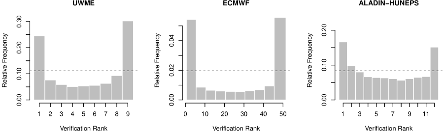
  (a) (b) (c)

Figure 1: Verification rank histograms. a) UWME for the calendar year 2008. b) ECMWF ensemble for the period May 1, 2010 – April 30, 2011; c) ALADIN-HUNEPS ensemble for the period April 1, 2012 – March 31, 2013.

Figure 1a shows the verification rank histogram of the raw ensemble, that is the histogram of ranks of validating observations with respect to the corresponding ensemble forecasts computed from the ranks at all locations and dates considered (see, e.g., Wilks,, 2011, Section 7.7.2). This histogram is strongly U-shaped as in many cases the ensemble members either underepredict or overpredict the validating observations. The reliability index  $\Delta=\sum_{i=1}^{c}\left|p_{i}-\frac{1}{c}\right|,$  where  $c$  denotes the number of classes in the histogram, each of which has expected relative frequency  $1/c$,  and  $p_{i}$  denotes the observed relative frequency in class  $i$, can be used to quantify the deviation of the rank distribution from uniformity (Delle Monache et al.,, 2006). For the UWME ensemble,  $\Delta$  equals $0.6508$, and the ensemble range contains the observed maximal wind speed in only $45.24\,\%$ of the cases (the nominal value of this coverage equals $7/9$, i.e $77.78\,\%$). Hence, the ensemble is under-dispersive, thus uncalibrated, and would require statistical post-processing to yield an improved forecast probability density function.

2.2 ECMWF ensemble

The global ensemble prediction system of the ECMWF consists of 50 exchangeable ensemble members which are generated from random perturbations in initial conditions and stochastic physics parametrization (Molteni et al.,, 1996; Leutbecher and Palmer,, 2008). Forecasts of near-surface (10 meter) wind speed for lead times up to 10 days ahead are issued twice a day at 00 UTC and 12 UTC, with a horizontal resolution of about 33 km. Following Lerch and Thorarinsdottir, (2013), we focus on the ECMWF ensemble run initialized at 00 UTC (2 am local time when DST operates and 1 am otherwise) and one day ahead forecasts. Predictions of daily maximum wind speed are obtained as the daily maximum of each ensemble member at each grid point location.

The verification is performed over a set of 228 synoptic observation stations over Germany. The validating observations are hourly observations of 10-minute average wind speed measured over the 10 minutes before the hour. Daily maximum wind speed observations are given by the maximum over the 24 hours corresponding to the time frame of the ensemble forecast. Ensemble forecasts at individual station locations are obtained by bilinear interpolation of the gridded model output. Our results are based on a verification period from May 1, 2010 to April 30, 2011, consisting of 83 220 individual forecast cases. Additional data from February 1, 2010 to April 30, 2011 are used to allow for training periods of equal lengths for all days in the verification period and for model selection purposes.

The verification rank histogram of the ECMWF ensemble displayed in Figure 1b is even more U-shaped than that of the UWME resulting in a reliability index of $1.1063$, while the ensemble range contains the validating observation just in $43.40\,\%$ of all cases (here the nominal value is $49/51$, that is $96.08\,\%$). Again, the ensemble is under-dispersive and statistical calibration is required.

2.3 ALADIN-HUNEPS ensemble

The ALADIN-HUNEPS system of the HMS covers a large part of continental Europe with a horizontal resolution of 12 km and is obtained with dynamical downscaling (by the ALADIN limited area model) of the global ARPEGE based PEARP system of Météo France (Horányi et al.,, 2006; Descamps et al.,, 2009). The ensemble consists of 11 members, 10 initialized from perturbed initial conditions and one control member from the unperturbed analysis, implying that the ensemble contains groups of exchangeable forecasts.

The data base contains 11 member ensembles of 42 hour forecasts for 10 meter instantaneous wind speed (given in m/s) for 10 major cities in Hungary (Miskolc, Szombathely, Győr, Budapest, Debrecen, Nyíregyháza, Nagykanizsa, Pécs, Kecskemét, Szeged) produced by the ALADIN-HUNEPS system of the HMS, together with the corresponding validating observations for the one-year period between April 1, 2012 and March 31, 2013. The validating observations were scrutinized by basic quality control algorithms including, e.g., consistency checks. The forecasts are initialized at 18 UTC (8 pm local time when DST operates and 7 pm otherwise). The data set is fairly complete since there are only six days when no forecasts are available. These dates are excluded from the analysis.

Similar to the previous two examples, the verification rank histogram of the raw ALADIN-HUNEPS ensemble is far from the desired uniform distribution (see Figure 1c), however, it shows a less under-dispersive character. The better fit of the ensemble can also be observed on its reliability index of $0.3217$ and coverage value of $61.21\,\%$, where the latter should be compared to the nominal coverage of $83.33\,\%$ ($10/12$).

3 Ensemble Model Output Statistics

As mentioned in the Introduction, the EMOS predictive PDF of a univariate weather quantity is a single parametric density function, where the parameters depend on the ensemble members. In case of temperature and pressure the normal distribution is a reasonable choice (Gneiting et al.,, 2005), while for non-negative variables such as wind speed, a skewed distribution is required. A popular candidate is the Weibull distribution (see, e.g., Justus et al.,, 1978), gamma or log-normal distributions are also in use (Garcia et al.,, 1988), while Thorarinsdottir and Gneiting, (2010) suggested an EMOS model based on truncated normal distribution with a cut-off at zero.

Let  $f_{1},f_{2},\ldots,f_{M}$  denote the ensemble of distinguishable forecasts of wind speed for a given location and time. This means that each ensemble member can be identified and tracked, which holds for example for the UWME (see Section 2.1).

However, most of the currently used ensemble prediction systems incorporate ensembles where at least some members are statistically indistinguishable. Such ensemble systems are usually producing initial conditions based on algorithms, which are able to find the fastest growing perturbations indicating the directions of the largest uncertainties. In most cases these initial perturbations are further enriched by perturbations simulating model uncertainties as well. Examples in the paper at hand are the ECMWF ensemble and the ALADIN-HUNEPS ensemble described in Sections 2.2 and 2.3, respectively. In such cases one usually has a control member (the one without any perturbation) and the remaining ensemble members forming one or two exchangeable groups.

In what follows, if we have  $M$  ensemble members divided into  $m$  exchangeable groups, where the  $k$th  group contains  $M_{k}\geq 1$  ensemble members ($\sum_{k=1}^{m}M_{k}=M$),  notation  $f_{k,\ell}$  is used for the $\ell$th member of the $k$th group.

3.1 Truncated normal model

Denote by  ${\mathcal{N}}^{\,0}\big{(}\mu,\sigma^{2}\big{)}$  the TN distribution with location  $\mu$,  scale  $\sigma>0$,  and cut-off at zero having PDF

$$g(x|\,\mu,\sigma):=\frac{\frac{1}{\sigma}\varphi\big{(}(x-\mu)/\sigma\big{)}}{\Phi\big{(}\mu/\sigma\big{)}},\quad x\geq 0,\qquad\text{and}\qquad g(x|\,\mu,\sigma):=0,\quad\text{otherwise,}$$

where  $\varphi$  and  $\Phi$  are the PDF and the cumulative distribution function (CDF) of the standard normal distribution, respectively. The EMOS predictive distribution of wind speed  $X$  proposed by Thorarinsdottir and Gneiting, (2010) is

$${\mathcal{N}}_{0}\big{(}a_{0}+a_{1}f_{1}+\cdots+a_{M}f_{M},b_{0}+b_{1}S^{2}\big{)}\qquad\text{with}\qquad S^{2}:=\frac{1}{M-1}\sum_{k=1}^{M}\big{(}f_{k}-\overline{f}\big{)}^{2},$$ (3.1)

where  $\overline{f}$  denotes the ensemble mean. Location parameters  $a_{0}\in{\mathbb{R}},\ a_{1},\ldots,a_{M}\geq 0$  and scale parameters  $b_{0},b_{1}\geq 0$  of model (3.1) can be estimated from the training data consisting of ensemble members and verifying observations from the preceding  $n$  days, by optimizing an appropriate verification score (see Section 3.5).

If the ensemble can be divided into groups of exchangeable members, ensemble members within a given group will get the same coefficient of the location parameter (Fraley et al.,, 2010) resulting in a predictive distribution of the form

$${\mathcal{N}}_{0}\bigg{(}a_{0}+a_{1}\sum_{\ell_{1}=1}^{M_{1}}f_{1,\ell_{1}}+\cdots+a_{m}\sum_{\ell_{m}=1}^{M_{m}}f_{m,\ell_{m}},b_{0}+b_{1}S^{2}\bigg{)},$$ (3.2)

where again,  $S^{2}$  denotes the ensemble variance. One might think of taking into account the grouping also in modelling the variance of the predictive PDF and use, e.g., the variance of the group means instead of the ensemble variance  $S^{2}$.  However, practical tests show that this (smaller) variance results in reduction of the predictive skill of the model.

3.2 Log-normal model

As an alternative to the TN model of Section 3.1 we propose an EMOS approach based on an LN distribution. This distribution has a heavier upper tail, and in this way it is more appropriate to model high wind speed values. The PDF of the LN distribution  $\mathcal{LN}\big{(}\mu,\sigma\big{)}$  with location  $\mu$  and shape  $\sigma>0$  is

$$h(x|\,\mu,\sigma):=\frac{1}{x\sigma}\varphi\big{(}(\log x-\mu)/\sigma\big{)},\quad x\geq 0,\qquad\text{and}\qquad h(x|\,\mu,\sigma):=0,\quad\text{otherwise,}$$ (3.3)

while the mean  $m$  and variance  $v$  of this distribution are

$$m={\mathrm{e}}^{\,\mu+\sigma^{2}/2}\qquad\text{and}\qquad v={\mathrm{e}}^{2\mu+\sigma^{2}}\big{(}{\mathrm{e}}^{\sigma^{2}}-1\big{)},\qquad\text{respectively.}$$

Further, since

$$\mu=\log\bigg{(}\frac{m^{2}}{\sqrt{v+m^{2}}}\bigg{)}\qquad\text{and}\qquad\sigma=\sqrt{\log\Big{(}1+\frac{v}{m^{2}}\Big{)}},$$ (3.4)

an LN distribution can also be parametrized by these quantities. In our EMOS approach  $m$  and  $v$  are affine functions of the ensemble members and ensemble variance, respectively, that is

$$m=\alpha_{0}+\alpha_{1}f_{1}+\cdots+\alpha_{M}f_{M}\qquad\text{and}\qquad v=\beta_{0}+\beta_{1}S^{2}.$$ (3.5)

Similar to the TN model, to obtain the values of mean and variance parameters  $\alpha_{0}\in{\mathbb{R}},\ \alpha_{1},\ldots,\alpha_{M}\geq 0$  and  $\beta_{0},\beta_{1}\geq 0$,  respectively, one has to perform an optimum score estimation based on some verification measure. Obviously, for the case of exchangeable ensemble members instead of (3.5) we have

$$m=\alpha_{0}+\alpha_{1}\sum_{\ell_{1}=1}^{M_{1}}f_{1,\ell_{1}}+\cdots+\alpha_{m}\sum_{\ell_{m}=1}^{M_{m}}f_{m,\ell_{m}}\qquad\text{and}\qquad v=\beta_{0}+\beta_{1}S^{2}.$$ (3.6)

3.3 Combined model

To combine the advantageous properties of TN and LN approaches, following Lerch and Thorarinsdottir, (2013), we also investigate a regime-switching method. Depending on the value of the ensemble median  $f_{med}$  we consider either a TN or an LN based EMOS model. Given a threshold  $\theta>0$,  the EMOS predictive distribution is  ${\mathcal{N}}^{\,0}\big{(}\mu_{TN},\sigma_{TN}^{2}\big{)}$  if  $f_{med}<\theta$  and  $\mathcal{LN}\big{(}\mu_{LN},\sigma_{LN}\big{)}$,  otherwise. Model parameters  $\mu_{TN}$  and  $\sigma_{TN}$  depend on the ensemble forecast according to (3.1) or (3.2), while the expressions for  $\mu_{LN}$  and  $\sigma_{LN}$  can be obtained form (3.5) or (3.6) via transformation (3.4). For training the combined model we propose two different methods. If the training data set is large enough, that is many forecast cases belong to each day to be investigated, the LN model is trained using only ensemble forecasts where  $f_{med}\geq\theta$,   while forecasts with ensemble median under the threshold are used to train the TN model. This technique is applied for calibrating the UWME and the ECMWF ensemble forecasts, see Sections 4.1 and 4.2, respectively. However, e.g., in case of the ALADIN-HUNEPS ensemble one has only 10 observation stations, so there are not enough data for separate training of the component models. In such situations one might utilize the same training data set both for the TN and for the LN predictive distribution and then choose between these two models according to the value of the ensemble median. This particular idea is applied in Section 4.3 for the ALADIN-HUNEPS forecasts.

3.4 General Extreme Value model

In Section 4 the predictive performances of the LN and TN-LN mixture models are compared to those of the GEV and TN-GEV mixture models of Lerch and Thorarinsdottir, (2013). The CDF of a GEV distribution  $\mathcal{GEV}\big{(}\mu,\sigma,\xi\big{)}$  with location  $\mu$,  scale  $\sigma>0$  and shape  $\xi$  equals

$$G(x|\,\mu,\sigma,\xi):=\begin{cases}\exp\Big{(}-\big{[}1+\xi(\frac{x-\mu}{\sigma})\big{]}^{-1/\xi}\Big{)},&\ \xi\neq 0;\\ \exp\Big{(}-\exp\big{(}-\frac{x-\mu}{\sigma}\big{)}\Big{)},&\ \xi=0,\end{cases}$$

if  $1+\xi(x-\mu)/\sigma>0$,  and zero otherwise. This definition shows the main disadvantage of using a GEV distribution for modelling wind speed, namely, there is a positive probability for a GEV distributed random variable to be negative.

For calibrating ECMWF ensemble forecasts of wind speed over Germany Lerch and Thorarinsdottir, (2013) suggest to model location and scale parameters by

$$\mu=\gamma_{0}+\gamma_{1}f_{1}+\cdots+\gamma_{K}f_{K}\qquad\text{and}\qquad\sigma=\sigma_{0}+\sigma_{1}\overline{f},$$ (3.7)

while the shape parameter  $\xi$  is considered to be independent of the ensemble. In general, one can also incorporate the ensemble variance into the models of location and scale . However, preliminary studies showed that model (3.7) is also a reasonable choice for the UWME and the ALADIN-HUNEPS ensemble. Further, the components of the TN-GEV mixture model for the various ensemble forecasts are trained as described in Section 3.2.

3.5 Parameter estimation

The aim of probabilistic forecasting is to obtain calibrated and sharp predictive distributions of future weather quantities (Gneiting et al.,, 2007). This goal should also be addressed in the choice of the scoring rule to be optimized in order to obtain the estimates of parameters of different EMOS models. For evaluating density forecasts the most popular scoring rules are the logarithmic score (Gneiting and Raftery,, 2007), i.e. the negative logarithm of the predictive PDF evaluated at the verifying observation, and the continuous ranked probability score (CRPS; Gneiting and Raftery,, 2007; Wilks,, 2011). Given a predictive CDF  $F(y)$  and an observation  $x$,  the CRPS is defined as

$$\mathop{\hbox{\rm CRPS}}\big{(}F,x\big{)}:=\int_{-\infty}^{\infty}\big{(}F(y)-{\mathbbm{1}}_{\{y\geq x\}}\big{)}^{2}{\mathrm{d}}y={\mathsf{E}}|X-x|-\frac{1}{2}{\mathsf{E}}|X-X^{\prime}|,$$ (3.8)

where  ${\mathbbm{1}}_{H}$  denotes the indicator of a set  $H$,  while  $X$  and  $X^{\prime}$  are independent random variables with CDF  $F$  and finite first moment. We remark that the CRPS can be expressed in the same unit as the observation. Both the logarithmic score and the CRPS are proper scoring rules which are negatively oriented, that is, the smaller the better. In this way the optimization with respect to the logarithmic score gives back the maximum likelihood (ML) estimates of the parameters.

Short calculation shows that the CRPS corresponding to the CDF  $\mathcal{G}$  of a TN distribution   ${\mathcal{N}}^{\,0}\big{(}\mu,\sigma^{2}\big{)}$  can be given in a closed form (see, e.g., Thorarinsdottir and Gneiting,, 2010), namely

$$\mathop{\hbox{\rm CRPS}}\big{(}\mathcal{G},x\big{)}=\sigma\bigg{[}\Phi\big{(}\mu/\sigma\big{)}\bigg{]}^{-2} \,\bigg{[}\frac{x-\mu}{\sigma}\Phi\big{(}\mu/\sigma\big{)}\Big{(}2\Phi\big{(}(x-\mu)/\sigma\big{)}+\Phi\big{(}\mu/\sigma\big{)}-2\Big{)}$$

$$+2\varphi\big{(}(y-\mu)/\sigma\big{)}\Phi\big{(}\mu/\sigma\big{)}-\frac{1}{\sqrt{\pi}}\Phi\big{(}\sqrt{2}\mu/\sigma\big{)}\bigg{]}.$$

In case of the LN model one faces a similar situation, straightforward calculations verify

$$\mathop{\hbox{\rm CRPS}}\big{(}\mathcal{H},x\big{)}\!=\!x\Big{[}2\Phi\big{(}(\log x\!-\!\mu)/\sigma\big{)}\!-\!1\Big{]}\!\!-\!2{\mathrm{e}}^{\mu+\sigma^{2}/2}\Big{[}\Phi\big{(}(\log x\!-\!\mu)/\sigma\!-\!\sigma\big{)}\!+\!\Phi\big{(}\sigma/\sqrt{2}\big{)}\!-\!1\Big{]},$$

where  $x\geq 0$  and  $\mathcal{H}$  is the CDF corresponding to the PDF (3.3) of   $\mathcal{LN}\big{(}\mu,\sigma\big{)}$.  Obviously, with the help of transformations (3.4),  $\mathop{\hbox{\rm CRPS}}\big{(}\mathcal{H},x\big{)}$  can also be expressed as a function of the mean  $m$  and variance  $v$  of the LN distribution $\mathcal{LN}\big{(}\mu,\sigma\big{)}$.

Now, following the ideas of Gneiting et al., (2005) and Thorarinsdottir and Gneiting, (2010), both for the TN and the LN model we estimate model parameters by minimizing the mean CRPS of the predictive distributions and validating observations corresponding to the forecast cases of the training period, while for the GEV model the ML method suggested by Lerch and Thorarinsdottir, (2013) is applied.

4 Results

As mentioned in the Introduction, the predictive performances of the LN model and of the TN-LN combined model (see Sections 3.2 and 3.3, respectively) are tested on the eight-member UWME, on the fifty-member ECMWF ensemble and on the ALADIN-HUNEPS ensemble of the HMS. The obtained results are compared to the fits of the TN, GEV and TN-GEV combined models investigated by Lerch and Thorarinsdottir, (2013), and to the verification scores of the raw ensemble. We also consider the scores corresponding to climatological forecasts which can be defined as forecasts calculated from observations in the training period used as an ensemble.

The goodness of fit of a calibrated forecast in terms of probability distributions is quantified with the help of the mean CRPS defined in Section 3.4. For the raw ensemble and climatology in (3.8) the empirical CDF replaces the EMOS predictive CDF. In order to evaluate forecasts for high wind speeds we also consider the threshold-weighted continuous ranked probability score (twCRPS)

$$\mathop{\hbox{\rm twCRPS}}\big{(}F,x\big{)}:=\int_{-\infty}^{\infty}\big{(}F(y)-{\mathbbm{1}}_{\{y\geq x\}}\big{)}^{2}\omega(y){\mathrm{d}}y$$

introduced by Gneiting and Ranjan, (2011), where  $\omega(y)\geq 0$  is a weight function. Obviously, case  $\omega(y)\equiv 1$  corresponds to the traditional CRPS defined by (3.8), while to address wind speeds above a given threshold  $r$  one may set  $\omega(y)={\mathbbm{1}}_{\{y\geq r\}}$.  In our study we consider threshold values approximately corresponding to the 90th, 95th and 99th percentiles of the wind speed observations. Further, in order to quantify the improvement in twCRPS with respect to a reference predictive CDF  $F_{ref}$  we make use of the threshold-weighted continuous ranked probability skill score (twCRPSS) defined as (see, e.g., Lerch and Thorarinsdottir,, 2013)

$$\mathop{\hbox{\rm twCRPSS}}\big{(}F,x\big{)}:=1-\frac{\mathop{\hbox{\rm twCRPS}}\big{(}F,x\big{)}}{\mathop{\hbox{\rm twCRPS}}\big{(}F_{ref},x\big{)}}.$$

This score is obviously positively oriented, and as a reference we always use the predictive CDF corresponding to the TN model.

Finally, for each EMOS model we investigate the coverage and average width of the central prediction interval corresponding to the nominal coverage of the raw ensemble (UWME: $77.78\,\%$; ECMWF: $96.08\,\%$; ALADIN-HUNEPS: $83.33\,\%$), where the coverage of a  $(1-\alpha)100\,\%,\ \alpha\in(0,1),$  central prediction interval is the proportion of validating observations located between the lower and upper  $\alpha/2$  quantiles of the predictive distribution. For a calibrated predictive PDF this value should be around  $(1-\alpha)100\,\%$  and the proposed choices of  $\alpha$  allow direct comparisons to the raw ensembles.

A continuous counterpart of the verification rank histogram (see Figure 1) of the raw ensemble is the probability integral transform (PIT) histogram of the predictive distribution. The PIT is the value of the predictive CDF evaluated at the verifying observation (Raftery et al.,, 2005), and the PIT histogram provides a good measure about the possible improvements of the under-dispersive character of the raw ensemble. The closer the histogram is to the uniform distribution, the better is the calibration.

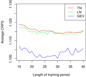
(a)

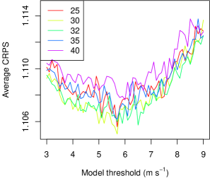
(b)

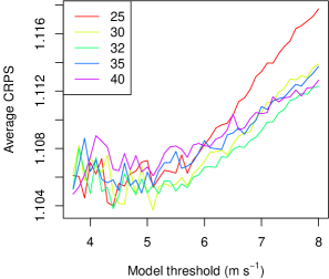
(c)

Figure 2: Mean CRPS values of the (a) EMOS predictive distributions for various training period lengths; (b) TN-LN mixture models corresponding to different training period lengths as functions of the threshold; (c) TN-GEV mixture models corresponding to different training period lengths as functions of the threshold for the UWME.

As point forecasts we consider EMOS and ensemble medians and means, which are evaluated with the use of mean absolute errors (MAEs) and root mean squared errors (RMSEs). Note that MAE is optimal for the median, while RMSE is optimal for the mean forecasts (Gneiting,, 2011; Pinson and Hagedorn,, 2012).

4.1 University of Washington Mesoscale Ensemble

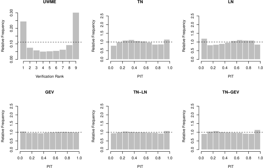
Figure 3: Verification rank histogram of the raw ensemble and PIT histograms of the EMOS post-processed forecasts for the UWME.

As the eight members of the UWME are non-exchangeable, the dependencies of location and scale parameters of the TN and GEV models on the ensemble members are specified by (3.1), (3.7), respectively, while the mean and variance of the LN model are linked to the ensemble according to (3.5).

As a first step we determine the optimal length of the rolling training period valid for all models and the optimal threshold values for TN-LN and TN-GEV mixtures. Figure 2a shows the mean CRPS values of all three models as functions of the training period length varying from 15 to 40 days. The mean CRPS of the GEV model takes its minimum at day 30 and this training period length seems reasonable for the other two models, too. This particular length of the training period is also supported by Figure 2b showing the mean CRPS values of the TN-LN mixture model as function of the threshold  $\theta$  for various training period lengths. For this mixture model the optimal threshold is $5.7$ m/s, while for the TN-GEV models similar arguments lead us to a threshold of $5.2$ m/s, see Figure 2c. Using these parameter values ensemble forecasts for the calendar year 2008 are calibrated. In case of the two regime-switching models an LN distribution is used in around one third, while a GEV distribution is applied in about 40 % of the 27 481 individual forecast cases.

Forecast		CRPS	twCRPS $(m/s)$			MAE	RMSE	Cover.	Av. w.
		$(m/s)$	$r\!=\!9$	$r\!=\!10.5$	$r\!=\!14$	$(m/s)$	$(m/s)$	$(\%)$	$(m/s)$
TN		1.114	0.150	0.074	0.010	1.550	2.048	78.65	4.67
LN		1.114	0.149	0.073	0.010	1.554	2.052	77.29	4.69
TN-LN,	$\!\!\!\!\theta\!=\!5.7$	1.105	0.149	0.073	0.010	1.550	2.050	77.73	4.64
GEV		1.100	0.145	0.072	0.010	1.554	2.047	77.20	4.69
TN-GEV,	$\!\!\!\!\theta\!=\!5.2$	1.105	0.145	0.072	0.010	1.555	2.055	77.20	4.60
Ensemble		1.353	0.175	0.085	0.011	1.655	2.169	45.24	2.53
Climatology		1.412	0.173	0.081	0.010	1.987	2.629	81.10	5.90

Table 1: Mean CRPS, mean twCRPS for various thresholds  $r$,  MAE of median and RMSE of mean forecasts and coverage and average width of $77.78\,\%$ central prediction intervals for the UWME.

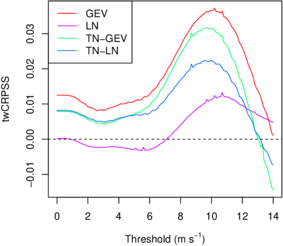
Figure 4: twCRPSS values for the UWME with TN as reference model.

Consider first the PIT histograms of the investigated EMOS models that are displayed in Figure 3. A comparison to the verification rank histogram of the raw ensemble shows that post-processing significantly improves the statistical calibration of the forecasts. However, one should admit that, e.g., the Kolmogorov-Smirnov test rejects the uniformity of PIT values in all cases, the highest $p$-value, corresponding to the GEV model, is $0.0049$.

In Table 1 scores for different probabilistic forecasts are given together with the average width and coverage of $77.75\,\%$ central prediction intervals. Verification measures of probabilistic forecasts and point forecasts calculated using TN, LN and GEV models and TN-LN ($\theta=5.7$ m/s) and TN-GEV ($\theta=5.2$ m/s) mixture models are compared to the corresponding measures calculated for the raw ensemble and climatological forecasts. By examining these results, one can clearly observe the obvious advantage of post-processing with respect to the raw ensemble or to the climatology. This is quantified in decrease of CRPS, MAE and RMSE values and in a significant improvement in the coverage of the $77.78\,\%$ central prediction intervals. On the other hand, the post-processed forecasts are less sharp than the ones calculated from the raw ensemble, however, this fact is coming from the small dispersion of the UWME, as also seen in the verification rank histogram of Figure 1a.

From the five competing models the GEV method produces the smallest CRPS and RMSE values and the lowest twCRPS scores for all three thresholds reported, while the best coverage and MAE value correspond to the TN-LN mixture model. However, the superiority of the GEV model is not surprising after examining Figure 4 showing the twCRPSS values of GEV, LN, TN-GEV and TN-LN EMOS methods with respect to the reference TN model as functions of the threshold. As the GEV model outperforms the TN model (and the other three, as well) at all investigated thresholds, combining the two methods does not result in an increase in the predictive skill. Hence, one can conclude that in case of the UWME data the GEV model has the best overall performance, but one should also remark that for this model the mean (maximal) probability of forecasting a negative wind speed is around $0.05\,\%\ (4\,\%)$.

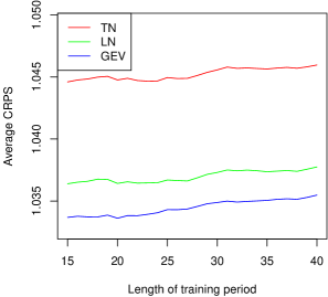
(a)

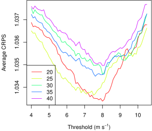
(b)

(c)

Figure 5: Mean CRPS values of the (a) EMOS predictive distributions for various training period lengths; (b) TN-LN mixture models corresponding to different training period lengths as functions of the threshold; (c) TN-GEV mixture models corresponding to different training period lengths as functions of the threshold for the ECMWF ensemble.

4.2 ECMWF ensemble

The ECMWF ensemble consists of one group of 50 exchangeable members. The parameters of the TN and the LN model are thus linked to the ensemble according to (3.2) and (3.6) with $m=1$. Following Lerch and Thorarinsdottir, (2013), the location and scale parameter of the GEV model are given as specified in (3.7) with $\gamma_{1},\dots,\gamma_{K}$ restricted to be equal.

To determine the optimal length of the training period for all models and the optimal model thresholds for the combination models we proceed as for the UWME ensemble and compute the average CRPS over a range of lengths of training periods and choices for the model threshold $\theta$, see Figure 5. Figure 5a suggests a training period of 20 days for all models, while Figures 5b and 5c suggest a model threshold of $\theta=8.0$ m/s and $\theta=7.3$ m/s for the TN-LN model and the TN-GEV model, respectively. With these threshold values, an LN distribution is used in around 14 % of the forecast cases in the verification set, and a GEV distribution is used in around 19 % of the forecast cases.

Figure 6: Verification rank histogram of the raw ensemble and PIT histograms of the EMOS post-processed forecasts.

Figure 6 showing the verification rank histogram of the raw ensemble and the PIT histograms of the various predictive distributions illustrates that all post-processing methods significantly increase the calibration of the ensemble. While the tails of the TN model appear to be slightly too light, the PIT histogram of the GEV model is gradually over-dispersive with minimally too heavy tails. The smallest deviations from uniformity are obtained for the LN model. The PIT histograms for the combination models resemble the PIT histogram of the TN model with small improvements at higher PIT values. Note that Kolmogorov-Smirnov tests reject the uniformity of the PIT values for all five models.

Forecast		CRPS	twCRPS $(m/s)$			MAE	RMSE	Cover.	Av.w.
		$(m/s)$	$r\!=\!10$	$r\!=\!12$	$r\!=\!15$	$(m/s)$	$(m/s)$	$(\%)$	$(m/s)$
TN		1.045	0.200	0.110	0.042	1.388	2.148	92.19	6.39
LN		1.037	0.198	0.109	0.042	1.386	2.138	93.16	6.91
TN-LN,	$\!\!\!\!\theta\!=\!8.0$	1.033	0.191	0.103	0.039	1.379	2.135	92.49	6.36
GEV		1.034	0.195	0.106	0.041	1.388	2.134	94.84	8.22
TN-GEV,	$\!\!\!\!\theta\!=\!7.3$	1.033	0.191	0.103	0.039	1.381	2.135	92.89	6.60
Ensemble		1.263	0.211	0.113	0.043	1.441	2.232	45.00	1.80
Climatology		1.550	0.251	0.128	0.045	2.144	2.986	95.84	11.91

Table 2: Mean CRPS, mean twCRPS for various thresholds  $r$,  MAE of median and RMSE of mean forecasts and coverage and average width of $96.08\,\%$ central prediction intervals for the ECMWF ensemble.

Table 2 summarizes the values of various scoring rules and coverage and average width of $96.08\,\%$ central prediction intervals. The raw ensemble forecasts outperform the climatological reference forecast and produce sharp prediction intervals, however, at the cost of being uncalibrated. All five post-processing methods significantly improve the calibration and predictive skill of the ensemble in terms of all scoring rules. The LN and the GEV model show small improvements over the TN model in terms of the average CRPS, MAE and RMSE. The best scores are obtained for the TN-LN and TN-GEV combination models. The TN-LN combination model achieves a minimally lower MAE and results in slightly narrower central prediction intervals. Further, the TN, LN and TN-LN models are strictly positive whereas the GEV and TN-GEV models occasionally assign small non-zero probabilities to negative wind speed observations. This effect is typically negligible as the average (maximum) probability mass assigned to negative wind speeds is smaller than 0.01 % (5 %) for the GEV model and smaller than 10^-7 % (0.001 %) for the TN-GEV model, respectively.

Figure 7: twCRPSS values for the ECMWF ensemble with TN as reference model.

To assess the predictive ability for high wind speed observations we also compute the twCRPS scores at different threshold values, see Table 2. The best scores in the upper tail are obtained by the TN-LN and TN-GEV combination models and the relative improvements over the TN model are considerably higher compared to the improvements in the unweighted CRPS. Figure 7 further shows the twCRPSS as a function of the threshold employed in the indicator weight function with the TN model as reference forecast. The twCRPSS is strictly positive for all models and threshold values, indicating improvements compared to the TN model. Except for the LN model, the twCRPSS of the models generally increases for larger threshold values and the greatest relative improvements over the TN model can be detected at threshold values around $15$ m/s. Despite the decreasing twCRPSS values of the LN model, the TN-LN model achieves the largest improvements over the TN model, closely followed by the TN-GEV model. Hence, one can conclude that the regime-switching models have the best overall performance showing almost the same predictive skills.

(a)

(b)

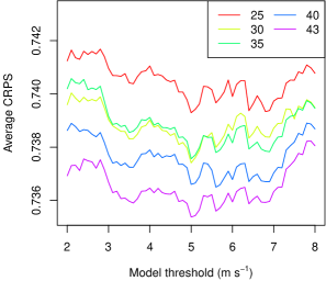
(c)

Figure 8: Mean CRPS values of the (a) EMOS predictive distributions for various training period lengths; (b) TN-LN mixture models corresponding to different training period lengths as functions of the threshold; (c) TN-GEV mixture models corresponding to different training period lengths as functions of the threshold for the ALADIN-HUNEPS ensemble.

4.3 ALADIN-HUNEPS ensemble

The way the ALADIN-HUNEPS ensemble is generated (see Section 2.3) induces a natural grouping of ensemble members into two groups. The first group contains just the control member, while in the second are the 10 statistically indistinguishable ensemble members initialized from randomly perturbed initial conditions. One should remark here that in Baran et al., (2013) a different grouping is also suggested (and later investigated in Baran, (2014) and Baran et al., (2014), too), where the odd and even numbered exchangeable ensemble members form two separate groups. This idea is justified by the method their initial conditions are generated, since only five perturbations are calculated and then they are added to (odd numbered members) and subtracted from (even numbered members) the unperturbed initial conditions. However, since in the present study the results corresponding to the two- and three-group models are rather similar, only the two-group case is reported.

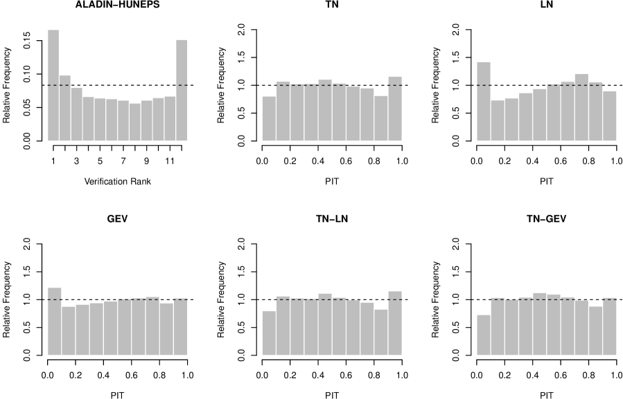
Figure 9: Verification rank histogram of the raw ensemble and PIT histograms of the EMOS post-processed forecasts for the ALADIN-HUNEPS ensemble.

A detailed earlier study of this particular data set (Baran et al.,, 2014) shows that in case of the TN distribution based EMOS model the optimal length of the rolling training period for ALADIN-HUNEPS wind speed forecasts is 43 days. Using this training period length one has a verification period between May 5, 2012 and March 31, 2013 containing 313 calendar days (3 130 forecast cases). In order to ensure the comparability of our results to the earlier studies by having the same verification period we keep the 43 days as the maximum possible training period length. However, based on Figure 8a showing the mean CRPS values of TN, LN and GEV models, respectively, as functions of the length of the training period, this maximal value of 43 days can also be accepted as optimal for all methods. Furthermore, this particular length is also supported by Figures 8b and 8c plotting the mean CRPS values of the TN-LN and TN-GEV mixture models as functions of the threshold  $\theta$  for various training period lengths. Based on these figures the optimal TN-LN and TN-GEV thresholds are $6.9$ m/s and $5$ m/s, while the corresponding percentages of usage of LN and GEV distributions in the mixtures are $4$ % and $15$ %, respectively.

EMOS model	TN	LN	TN-LN	GEV	TN-GEV
$p$-value	$0.127$	$4.42\!\times\!10^{-6}$	$0.117$	$0.070$	$0.014$

Table 3: $p$-values of Kolmogorov-Smirnov tests for uniformity of PIT values for the ALADIN-HUNEPS ensemble.

Similar to the previous two sections we first consider the PIT histograms of all considered EMOS models, displayed in Figure 9. Compared to the verification rank histogram of the raw ensemble all post-processing methods result in a significant improvement in the goodness of fit to the uniform distribution, while from the competing calibration methods the TN and the TN-LN mixture models have the best performance. This latter statement is justified by the $p$-values of Kolmogorov-Smirnov tests for uniformity given in Table 3.

Forecast		CRPS	twCRPS $(m/s)$			MAE	RMSE	Cover.	Av.w.
		$(m/s)$	$r\!=\!6$	$r\!=\!7$	$r\!=\!9$	$(m/s)$	$(m/s)$	$(\%)$	$(m/s)$
TN		0.738	0.102	0.054	0.012	1.037	1.357	83.59	3.53
LN		0.741	0.102	0.054	0.011	1.038	1.362	80.44	3.57
TN-LN,	$\!\!\!\!\theta\!=\!6.9$	0.737	0.101	0.054	0.011	1.035	1.356	83.59	3.54
GEV		0.737	0.098	0.052	0.011	1.041	1.355	81.21	3.54
TN-GEV,	$\!\!\!\!\theta\!=\!5.0$	0.735	0.098	0.052	0.011	1.039	1.355	85.59	3.72
Ensemble		0.803	0.112	0.059	0.013	1.069	1.373	68.22	2.88
Climatology		1.046	0.127	0.064	0.012	1.481	1.922	82.54	3.43

Table 4: Mean CRPS, mean twCRPS for various thresholds  $r$,  MAE of median and RMSE of mean forecasts and coverage and average width of $83.33\,\%$ central prediction intervals for the ALADIN-HUNEPS ensemble.

Similar to Sections 4.1 and 4.2 in Table 4 verification scores for probabilistic forecasts and the average width and coverage of $83.33\,\%$ central prediction intervals are reported. Compared to the raw ensemble and to climatology post-processed forecasts show the same behaviour as before: improved predictive skills and better calibration. The lowest CRPS and RMSE values belong to the TN-GEV mixture model, while the TN-LN regime-switching method provides the best MAE score and coverage combined with a rather narrow central prediction interval. Further, for $6$ m/s and $7$ m/s threshold values the GEV and TN-GEV models result in slightly lower twCRPS scores than the TN-LN mixture, while for $r=9$ m/s this advantage practically disappears. This phenomenon can also be observed in Figure 10 showing the twCRPSS values of the GEV, LN, TN-GEV and TN-LN methods with respect to the reference TN model as functions of the threshold. Finally, the mean (maximal) probabilities of predicting a negative wind speed by the GEV and TN-GEV methods are $0.33\,\%$ ($9.46\,\%$) and $2.74\times 10^{-3}\,\%$ ($0.15\,\%$), respectively. Taking also into account the goodness of fit of PIT histograms (see Table 3) one can conclude that for ALADIN-HUNEPS wind speed forecasts the TN-LN mixture model has the best overall performance.

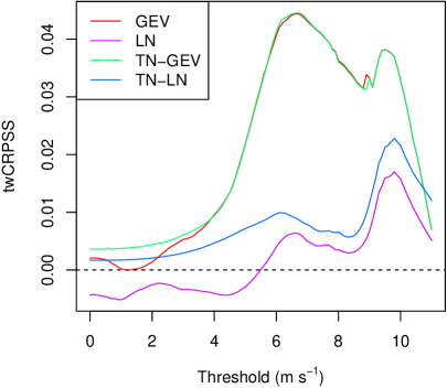
Figure 10: twCRPSS values for the ALADIN-HUNEPS ensemble with TN as reference model.

5 Conclusions

We introduce a new EMOS model for calibrating ensemble forecasts of wind speed providing a predictive PDF which follows a log-normal distribution. In order to have better forecasts in the tails we also consider a regime-switching approach based on the ensemble median, which considers a truncated normal EMOS model for low values and a log-normal EMOS for the high ones. The two approaches are tested on wind speed forecasts of the eight-member University of Washington mesoscale ensemble, of the fifty-member ECMWF ensemble and of the eleven-member ALADIN-HUNEPS ensemble of the Hungarian Meteorological Service. These ensemble prediction systems differ both in the wind speed quantities being forecasted and in the generation of the ensemble members. Using appropriate verification measures (CRPS of probabilistic, MAE of median and RMSE of mean forecasts, coverage and average width of central prediction intervals corresponding to the nominal coverage, twCRPS corresponding to 90th, 95th and 99th percentiles of the verifying observations) the predictive performances of the LN and TN-LN mixture models are compared to those of the TN based EMOS method (Thorarinsdottir and Gneiting,, 2010), of the GEV and TN-GEV mixture models (Lerch and Thorarinsdottir,, 2013), of the raw ensemble, and of the climatological forecasts as well. From the results of the presented case studies one can conclude that compared to the raw ensemble and to climatology post-processing always improves the calibration of probabilistic and accuracy of point forecasts. Further, the TN-LN mixture model outperforms the traditional TN method (Thorarinsdottir and Gneiting,, 2010) and it is at least able to keep up with the models utilizing the GEV distribution (Lerch and Thorarinsdottir,, 2013) without the problem of forecasting negative wind speed values.

Acknowledgments.    Essential part of this work was made during the visit of Sándor Baran at the Heidelberg Institute of Theoretical Studies. Sebastian Lerch gratefully acknowledges support by the Volkswagen Foundation within the program “Mesoscale Weather Extremes – Theory, Spatial Modelling and Prediction (WEX-MOP).” Sándor Baran was supported by the Campus Hungary Program and by the TÁMOP-4.2.2.C-11/1/KONV-2012-0001 project. The project has been supported by the European Union, co-financed by the European Social Fund. The authors are indebted to Tilmann Gneiting for his useful suggestions and remarks, to the University of Washington MURI group for providing the UWME data and to Mihály Szűcs from the HMS for the ALADIN-HUNEPS data.

References

- Baran, (2014) Baran, S. (2014) Probabilistic wind speed forecasting using Bayesian model averaging with truncated normal components. Comput. Stat. Data. Anal. 75, 227–238.
- Baran et al., (2013) Baran, S., Horányi, A. and Nemoda, D. (2013) Statistical post-processing of probabilistic wind speed forecasting in Hungary. Meteorol. Z. 22, 273–282.
- Baran et al., (2014) Baran, S., Horányi, A. and Nemoda, D. (2014) Comparison of BMA and EMOS statistical calibration methods for temperature and wind speed ensemble weather prediction. Időjárás, in press.
- Bouallègue et al., (2013) Bouallègue, B. Z., Theis, S. and Gebhardt, C. (2013) Enhancing COSMO-DE ensemble forecasts by inexpensive techniques. Meteorol. Z. 22, 49–59.
- Buizza et al., (2005) Buizza, R., Houtekamer, P. L., Toth, Z., Pellerin, G., Wei, M. and Zhu, Y. (2005) A comparison of the ECMWF, MSC, and NCEP global ensemble prediction systems. Mon. Wea. Rev. 133, 1076–1097.
- Buizza et al., (1993) Buizza, R., Tribbia, J., Molteni, F. and Palmer, T. (1993) Computation of optimal unstable structures for a numerical weather prediction system. Tellus A 45, 388–407.
- Delle Monache et al., (2006) Delle Monache, L., Hacker, J. P., Zhou, Y., Deng, X. and Stull, R. B. (2006) Probabilistic aspects of meteorological and ozone regional ensemble forecasts. J. Geophys. Res. 111 D24307, doi: 10.1029/2005JD006917.
- Descamps et al., (2009) Descamps, L., Labadier, C., Joly, A. and Nicolau, J. (2009) Ensemble Prediction at Météo France (poster introduction by Olivier Riviere) 31st EWGLAM and 16th SRNWP meetings, 28th September – 1st October, 2009. Available at: http://srnwp.met.hu/Annual_Meetings/2009/download/sept29/morning/posterpearp.pdf
- Eckel and Mass, (2005) Eckel, F. A. and Mass, C. F. (2005) Effective mesoscale, short-range ensemble forecasting. Wea. Forecasting 20, 328–350.
- ECMWF Directorate, (2012) ECMWF Directorate (2012) Describing ECMWF’s forecasts and forecasting system. ECMWF Newsletter 133, 11–13.
- Fraley et al., (2010) Fraley, C., Raftery, A. E. and Gneiting, T. (2010) Calibrating multimodel forecast ensembles with exchangeable and missing members using Bayesian model averaging. Mon. Wea. Rev. 138, 190–202.
- Fraley et al., (2009) Fraley, C., Raftery, A. E., Gneiting, T. and Sloughter, J. M. (2009) EnsembleBMA: An R package for probabilistic forecasting using ensembles and Bayesian model averaging. Technical Report 516R, Department of Statistics, University of Washington. Available at: www.stat.washington.edu/research/reports/2008/tr516.pdf
- Fraley et al., (2011) Fraley, C., Raftery, A. E., Gneiting, T., Sloughter, J. M. and Berrocal, V. J. (2011) Probabilistic weather forecasting in R. The R Journal 3, 55–63.
- Garcia et al., (1988) Garcia, A., Torres, J. L., Prieto, E. and De Francisco, A. (1998) Fitting wind speed distributions: A case study. Sol. Energ. 62, 139–144.
- Gebhardt et al., (2011) Gebhardt, C., Theis, S. E., Paulat, M. and Bouallègue, Z. B. (2011) Uncertainties in COSMO-DE precipitation forecasts introduced by model perturbations and variation of lateral boundaries. Atmos. Res. 100, 168–177.
- Gneiting, (2011) Gneiting, T. (2011) Making and evaluating point forecasts. J. Amer. Statist. Assoc. 106, 746–762.
- Gneiting, (2014) Gneiting, T. (2014) Calibration of medium-range weather forecasts. ECMWF Technical Memorandum No. 719. Available at: old.ecmwf.int/publications/library/ecpublications/ _pdf/tm/701-800/tm719.pdf
- Gneiting et al., (2007) Gneiting, T., Balabdaoui, F. and Raftery, A. E. (2007) Probabilistic forecasts, calibration and sharpness. J. Roy. Stat. Soc. B. 69, 243–268.
- Gneiting and Raftery, (2005) Gneiting, T. and Raftery, A. E. (2005) Weather forecasting with ensemble methods. Science 310, 248–249.
- Gneiting and Raftery, (2007) Gneiting, T. and Raftery, A. E. (2007) Strictly proper scoring rules, prediction and estimation. J. Amer. Statist. Assoc. 102, 359–378.
- Gneiting et al., (2005) Gneiting, T., Raftery, A. E., Westveld, A. H. and Goldman, T. (2005) Calibrated probabilistic forecasting using ensemble model output statistics and minimum CRPS estimation. Mon. Wea. Rev. 133, 1098–1118.
- Gneiting and Ranjan, (2011) Gneiting, T. and Ranjan, R. (2011) Comparing density forecasts using threshold- and quantile-weighted scoring rules. J. Bus. Econ. Stat. 29, 411–422.
- Grell et al., (1995) Grell, G. A., Dudhia, J. and Stauffer, D. R. (1995) A description of the fifth-generation Penn state/NCAR mesoscale model (MM5). Technical Note NCAR/TN-398+STR. National Center for Atmospheric Research, Boulder. Available at: http://www.mmm.ucar.edu/mm5/documents/mm5-desc-doc.html
- Hágel, (2010) Hágel, E. (2010) The quasi-operational LAMEPS system of the Hungarian Meteorological Service. Időjárás 114, 121–133.
- Horányi et al., (2006) Horányi, A, Kertész, S., Kullmann, L. and Radnóti, G. (2006) The ARPEGE/ALADIN mesoscale numerical modelling system and its application at the Hungarian Meteorological Service. Időjárás 110, 203–227.
- Horányi et al., (2011) Horányi, A., Mile, M., Szűcs, M. (2011) Latest developments around the ALADIN operational short-range ensemble prediction system in Hungary. Tellus A 63, 642–651.
- Justus et al., (1978) Justus, C. G., Hargraves, W. R., Mikhail, A. and Graber, D. (1978) Methods for estimating wind speed frequency distributions. J. Appl. Meteor. 17, 350–353.
- Leith, (1974) Leith, C. E. (1974) Theoretical skill of Monte-Carlo forecasts. Mon. Wea. Rev. 102, 409–418.
- Lerch and Thorarinsdottir, (2013) Lerch, S. and Thorarinsdottir, T. L. (2013) Comparison of non-homogeneous regression models for probabilistic wind speed forecasting. Tellus A 65, 21206.
- Leutbecher and Palmer, (2008) Leutbecher, M. and Palmer, T. N. (2008) Ensemble forecasting. J. Comp. Phys. 227, 3515–3539.
- Molteni et al., (1996) Molteni, F., Buizza, R. and Palmer, T. N. (1996) The ECMWF Ensemble Prediction System: Methodology and validation. Q. J. R. Meteorol. Soc. 122, 73–119.
- Möller et al., (2013) Möller, A., Lenkoski, A. and Thorarinsdottir, T. L. (2013) Multivariate probabilistic forecasting using ensemble Bayesian model averaging and copulas. Q. J. R. Meteorol. Soc. 139, 982–991.
- National Weather Service, (1998) National Weather Service (1998) Automated Surface Observing System (ASOS) User’s Guide. Available at: http://www.weather.gov/asos/aum-toc.pdf
- Pinson and Hagedorn, (2012) Pinson, P. and Hagedorn, R. (2012) Verification of the ECMWF ensemble forecasts of wind speed against analyses and observations. Meteorol. Appl. 19, 484–500.
- Raftery et al., (2005) Raftery, A. E., Gneiting, T., Balabdaoui, F. and Polakowski, M. (2005) Using Bayesian model averaging to calibrate forecast ensembles. Mon. Wea. Rev. 133, 1155–1174.
- Sloughter et al., (2010) Sloughter, J. M., Gneiting, T. and Raftery, A. E. (2010) Probabilistic wind speed forecasting using ensembles and Bayesian model averaging. J. Amer. Stat. Assoc. 105, 25–37.
- Thorarinsdottir and Gneiting, (2010) Thorarinsdottir, T. L. and Gneiting, T. (2010) Probabilistic forecasts of wind speed: Ensemble model output statistics by using heteroscedastic censored regression. J. Roy. Statist. Soc. Ser. A 173, 371–388.
- Toth and Kalnay, (1997) Toth, Z. and Kalnay, E. (1997) Ensemble forecasting at NCEP and the breeding method. Mon. Wea. Rev. 125, 3297–3319.
- Wilks, (2011) Wilks, D. S. (2011) Statistical Methods in the Atmospheric Sciences. 3rd ed., Elsevier, Amsterdam.
- Williams et al., (2014) Williams, R. M., Ferro, C. A. T. and Kwasniok, F. (2014) A comparison of ensemble post-processing methods for extreme events. Q. J. R. Meteorol. Soc. 140, 1112–1120.