Abstract

The objective of this work is to present the effects of a nonminimally coupled model of gravity on a Solar System short range regime. For this reason, this study is only valid when the cosmological contribution is considered irrelevant. The action functional of the model involves two functions $f^{1}(R)$ and $f^{2}(R)$ of the Ricci scalar curvature $R$, where the last one multiplies the matter Lagrangian.

Using a Taylor expansion around $R=0$ for both functions $f^{1}(R)$ and $f^{2}(R)$, it was found that the metric around a spherical object is a perturbation of the weak-field Schwarzschild metric. The $tt$ component of the metric, a Newtonian plus a Yukawa perturbation term, is constrained using the available observational results.

First it is shown that this effect is null when the characteristic mass scales of each function $f^{1}(R)$ and $f^{2}(R)$ are identical. Besides, the conclusion is that the nonminimal coupling only affects the Yukawa contribution strength and not its range and that the Starobinsky model for inflation is not experimentally constrained. Moreover, the geodetic precession effect, obtained also from the radial perturbation of the metric, reveals to be of no relevance for the constraints.

The original work presented in this thesis closely follows Ref. [1].

todaythesis[]

O objectivo deste trabalho é apresentar os efeitos de um modelo de acoplamento não-mínimo da gravidade no Sistema Solar, num regime de curto alcance. Por esta razão, este estudo só é válido quando a contribuição cosmológica é considerada irrelevante. A acção do modelo inclui duas funções $f^{1}(R)$ e $f^{2}(R)$ da curvatura escalar de Ricci $R$, onde a segunda multiplica o Lagrangeano da matéria.

Através de uma expansão de Taylor em torno de $R=0$ para ambas as funções $f^{1}(R)$ e $f^{2}(R)$, descobriu-se que a métrica à volta de um objecto esférico é uma perturbação da aproximação de campo fraco da métrica de Schwarzschild. A componente $tt$ da métrica, um termo Newtoniano com um termo perturbativo de Yukawa, é condicionada através dos resultados observacionais disponíveis.

Em primeiro lugar, verifica-se que este efeito é anulado quando as escalas de massa características de cada função $f^{1}(R)$ e $f^{2}(R)$ são idênticas. Para além disto, a conclusão é que o acoplamento não-mínimo só afecta a força da contribuição de Yukawa e não o seu alcance e que o modelo de Starobinsky para a inflação não está limitado experimentalmente. Mais ainda, o efeito da precessão geodética, obtida também da perturbação radial da métrica, revela não ter relevância para os limites obtidos.

O trabalho original apresentado nesta tese segue ao pormenor a Ref. [1].

Teorias $f(R)$; Acoplamento não mínimo; Modificações Yukawa à lei do quadrado inverso; Sistema Solar

Abbreviations

GR

General Relativity

EFE

Einstein Field Equations

FLRW

Friedmann-Lemaître-Robertson-Walker

EOS

equation of state

BD

Brans-Dicke

SRA

Slow-Roll Approximation

NMC

nonminimal coupling

WMAP

Wilkinson Microwave Anisotropy Probe

CMB

Cosmic Microwave Background

ISL

Inverse-Square Law

PPN

Parametrized Post-Newtonian

GPB

Gravity Probe B

LLR

Lunar Laser Ranging

Chapter 1 Introduction

1.1 General Relativity

To study gravity, physicists rely on the theory of General Relativity (GR), as they have done for almost a hundred years. GR was developed by Einstein in 1916 and since then it has been able to demonstrate itself as a solid theory of physics. After its theoretical framework was developed, the observational confirmations didn’t take long to appear: several experiments have been done to confirm it [2], such as the measure of the perihelion of Mercury, the detection of the bending of light or the Eötvös torsion balances experiment, just to name a few of the classics. Besides these, also today there are people working on very recent General Relativity tests and its most dramatic consequences, such as the LAGEOS [3] and Lunar Laser Ranging [4] collaborations.

One of the main tenets of GR is the relation between matter and geometry, where gravity appears not as a force field but as a deformation of the spacetime. This is mathematically represented in the Einstein Field Equations (EFE), which, as all field equations in physics, are obtained from an action principle. Indeed, consider the Einstein-Hilbert action

$$S=\int\left[\kappa\left(R-2\Lambda\right)+{\cal L}_{m}\right]\sqrt{-g}\text{ d}^{4}x,$$ (1.1)

where $R$ is the Ricci scalar, ${\cal L}_{m}$ is the matter lagrangian, $\Lambda$ stands for the Cosmological Constant, $g$ is the determinant of the metric and $\kappa$ is defined as $\kappa=c^{4}/(16\pi G)$, with $G$ as Newton’s constant of gravity and $c$ as the velocity of light in a vacuum.

Hence, by the principle of least action, the variation of the action $\delta S=0$ with respect to the metric $g^{\mu\nu}$ yields the EFE,

$$G_{\mu\nu}+\Lambda g_{\mu\nu}=\dfrac{1}{2\kappa}T_{\mu\nu},$$ (1.2)

where $G_{\mu\nu}\equiv R_{\mu\nu}-\dfrac{1}{2}g_{\mu\nu}R$ is the Einstein tensor and $T_{\mu\nu}$ is the energy-momentum tensor of matter, clearly showing the already stated relation between matter and geometry. Applying the Bianchi identities, it is found that these equations satisfy the conservation of energy,

$$\nabla^{\mu}G_{\mu\nu}=0\Rightarrow\nabla^{\mu}T_{\mu\nu}=0.$$ (1.3)

1.2 Standard Cosmology and Inflation

Following the Cosmological Principle, which states that the universe is homogeneous and isotropic, the universe can be said to have a Friedmann-Lemaître-Robertson-Walker (FLRW) metric [5, 6]:

$$ds^{2}=-c^{2}dt^{2}+a^{2}(t)\left(\dfrac{dr^{2}}{1-Kr^{2}}+r^{2}d\Omega^{2}\right),$$ (1.4)

where $a(t)$ is the cosmological scale factor, $d\Omega^{2}$ is the line element for the 2-sphere and $K$ is related to the curvature of the spatial section of spacetime, where the spatial coordinates are comoving coordinates.

One may consider that at very large scales the universe can be described as being a perfect fluid, endowed with an energy-momentum tensor

$$T_{\mu\nu}=\left(\rho+\dfrac{p}{c^{2}}\right)u_{\mu}u_{\nu}+pg_{\mu\nu},$$ (1.5)

where $\rho$ is the energy density, $p$ is the pressure and $u_{\mu}$ is the 4-velocity vector. Inserting this tensor and the metric (1.4) into the EFE (1.2) gives the cosmology structure equations:

$$\dot{a}^{2}+Kc^{2} = \dfrac{a^{2}}{3}\left(8\pi G\rho+\Lambda c^{2}\right),$$ (1.6)

$$\dfrac{\ddot{a}}{a} = -\dfrac{4\pi G}{3}\left(\rho+\dfrac{3p}{c^{2}}\right)+\dfrac{\Lambda c^{2}}{3},$$ (1.7)

where $\dot{a}=da/dt$. The first of these equations is called the Friedmann equation. Through a simple manipulation, both these equations can be written in the form of the conservation of energy:

$$\dot{\rho}+3H\left(\rho c^{2}+p\right)\Leftrightarrow\dfrac{d}{dt}\left(\rho c^{2}a^{3}\right)+p\dfrac{d}{dt}a^{3}=0,$$ (1.8)

which can also be directly obtained from Eq. (1.3). The Hubble parameter is extremely useful to characterize the evolution of the universe and is defined as

$$H=\dot{a}/a.$$ (1.9)

The above equations (1.6) and (1.7) yield a full description of the structure and development of the universe if an equation of state (EOS) is known. The simplest approach is to consider a barotrope, described by the equation

$$p=w\rho,$$ (1.10)

where $w$ is a constant independent of time. Notice that inserting this EOS into the conservation of energy (1.8) yields

$$\dfrac{\dot{\rho}}{\rho}=-3\left(1+w\right)H.$$ (1.11)

This expression can be integrated to obtain the solution of $\rho$,

$$\rho(a)=\rho_{0}a^{-3\left(1+w\right)},$$ (1.12)

where $\rho_{0}$ is the value of the energy density at the present time $t_{0}$, when $a(t_{0})\equiv a_{0}$.

The universe underwent different stages of evolution, characterized by the dominance of different kinds of matter, in the so-called radiation, matter and dark energy eras. In the radiation era the Universe was dominated by electromagnetic radiation or massive particles travelling at velocities close to the speed of light, so that its EOS is

$$p_{r}=\dfrac{1}{3}\rho_{r}.$$ (1.13)

The energy density in the radiation era falls off as $\rho_{r}\propto a^{-4}$. As for the matter era, dominated by nonrelativistic particles with approximately no collisions, matter has essentially zero pressure $p_{m}=0$, so that $w_{m}=0$. In this case the energy density falls off as $\rho_{m}\propto a^{-3}$.

Knowing how the energy density behaves with the scale factor, it is possible to derive the function $a(t)$ through the Friedmann equation (1.6) and the Hubble parameter definition (1.9). Considering a flat model $K=0$ with $\Lambda=0$, in the radiation era the scale factor becomes $a(t)\propto t^{1/2}$ and in the matter era, $a(t)\propto t^{2/3}$. It should also be mentioned that when a non-vanishing cosmological constant $\Lambda\neq 0$ dominates, so that $\rho_{\Lambda}=-p_{\Lambda}$ (i.e. $\omega_{\Lambda}=-1$), one obtains $\rho_{\Lambda}\propto a$, so that $a(t)\propto\exp(Ht)$. When the universe behaves according to the latter model it means that it is going through a De Sitter phase, which characterizes the dark energy era.

The standard Big-Bang model, described by Eqs. (1.7) and (1.6), has seen many of its predictions confirmed by cosmological observations, such as the galaxies red-shift or the detection of the Cosmic Microwave Background (CMB) [7]. Nonetheless, some observations showed that there were three problems in this model. They were the horizon problem, related to the explanation of how regions of the universe not causally related were in thermal equilibrium, as shown by the CMB Radiation, the flatness problem, from the extreme fine-tuning necessary to explain how the universe is as spatially flat as it looks, and the monopole problem, indicating that these exotic entities should dominate the universe in the present time, contrary to observations. These three problems were solved in a single theory, called inflation [8].

The theory of inflation comes directly from the solution to the flatness problem. Defining the critical density as

$$\rho_{c}(t)=3H^{2}/8\pi G,$$ (1.14)

and neglecting the cosmological constant term, the Friedmann equation (1.6) can be written as

$$\left|\Omega-1\right|=\dfrac{|K|c^{2}}{a^{2}H^{2}}=\dfrac{\left|K\right|c^{2}}{\dot{a}^{2}},$$ (1.15)

where $\Omega$ is the density parameter defined as $\Omega=\rho/\rho_{c}$. The standard cosmological model predicts that the $r.h.s.$ of the above equation should increase with time, hence $\Omega$ should become larger with time since the Big Bang, but observations yield an $\Omega\sim 1$, i.e. the universe is flat ($K=0$). The only way to counter this would be for the $r.h.s.$ to decrease with time:

$$\dfrac{\left|K\right|c^{2}}{\dot{a}^{2}}\text{ should decrease }\Rightarrow\dot{a}\text{ should increase }\Rightarrow\ddot{a}>0,$$ (1.16)

which is the inflation condition.

The origin of inflation is explained by means of a scalar field named inflaton, $\phi$, whose effective energy density and pressure are written as

$$\rho_{\phi}=\dfrac{\dot{\phi}^{2}}{2}+V(\phi),\qquad\qquad\qquad p_{\phi}=\dfrac{\dot{\phi}^{2}}{2}-V(\phi),$$ (1.17)

where the potential $V(\phi)$ depends on the inflation model in question. Moreover, the inflation condition means that the potential energy must dominate in order to obtain a phase of accelerated expansion,

$$\ddot{a}>0\Leftrightarrow p<-\rho c^{2}/3\Leftrightarrow\dot{\phi}^{2}<V(\phi),$$ (1.18)

where the second cosmology structure equation (1.7) was used. This is the so-called Slow-Roll Approximation (SRA), which states that the kinetic term can be neglected with respect to the potential term. Notice that if this condition applies, then by Eq. (1.17), the EOS becomes similar to that of a Cosmological Constant, $\rho_{\phi}\simeq-p_{\phi}$. Inserting the inflaton energy density and pressure (1.17) into the Friedmann equation (1.6) and the energy conservation (1.8) gives the inflation structure equations:

$$H^{2} = \dfrac{8\pi G}{3}\left[V(\phi)+\dfrac{\dot{\phi}^{2}}{2}\right],$$ (1.19)

$$\ddot{\phi}+3H\dot{\phi} = -V^{\prime}(\phi),$$ (1.20)

where $V^{\prime}(\phi)=dV/d\phi$. By the SRA, these equations become

$$H^{2} \simeq \dfrac{8\pi G}{3}V(\phi),$$ (1.21)

$$3H\dot{\phi} \simeq -V^{\prime}(\phi).$$ (1.22)

It is also possible to define the slow-roll parameters as

$$\epsilon(\phi) = \dfrac{1}{16\pi G}\left(\dfrac{V^{\prime}}{V}\right)^{2}\ll 1,$$ (1.23)

$$\left|\eta(\phi)\right| = \left|\dfrac{1}{8\pi G}\dfrac{V^{\prime\prime}}{V}\right|\ll 1,$$ (1.24)

which measure the slope and the curvature of $V(\phi)$, respectively. Their smallness is necessary to satisfy the SRA.

The number of $e$-folds between an initial $\phi_{i}$ and final state $\phi_{f}$ of the inflation is determined by

$$N=\ln\dfrac{a(t_{f})}{a(t_{i})}=\int^{t_{f}}_{t_{i}}Hdt=-8\pi G\int^{\phi_{f}}_{\phi_{i}}\dfrac{V}{V^{\prime}}d\phi,$$ (1.25)

where $dt=d\phi/\dot{\phi}$ was used. It is known that for inflation to overcome the three original problems of the standard cosmological model, $N$ should be no less than $70$ [9].

The duration of inflation is the time when the SRA is valid, a period in which the energy density and temperature of the universe are extremely low. As such, at the end of inflation, the potential $V(\phi)$ loses its strength and the universe must go through a reheating process, as the exponential expansion has left the Universe at essentially zero temperature. This is achieved through an oscillation of the inflaton in a potential well, as shown in figure 1.1.

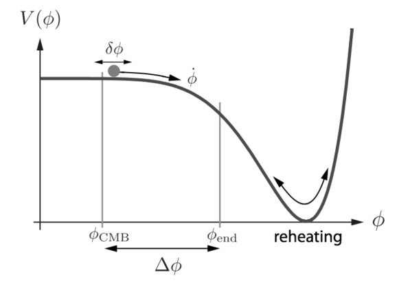
Figure 1.1: Typical inflation potential. Adapted from Ref. [10].

Quantum field theory explains that an oscillating electric field produces electron-positron pairs; similarly, the oscillation of the field $\phi$ produces its own particles, with the energy that it is losing until the end of the oscillations. This will happen until the temperature needed to go back to the standard cosmological model is reached. Such a process is explained in a more analytical way through the conservation of energy inflation equation (1.20), by adding the term $\Gamma_{\phi}$, which is the decay range of $\phi$:

$$\ddot{\phi}+3H\dot{\phi}+\Gamma_{\phi}\dot{\phi}+V^{\prime}(\phi)=0.$$ (1.26)

This can be interpreted as a friction term, where the energy lost by the inflaton is transferred to the particles produced, thus reheating the Universe.

Without entering into much details, inflation has already some observational evidences, such as the last year results from the Planck experiment [11] and the very recent clues of evidence of gravitational waves [12] (although some doubts have arisen as to the validity of these findings [13, 14]).

1.3 Modern Problems

Besides the exact origins of inflation, other problems still remain to be explained, such as the relation between quantum mechanics and gravity (check Ref. [15] for a review on the subject) and the nature of dark matter and dark energy. These concepts arise as an explanation to an observational effect that is contrary to the theoretical prevision of GR. Dark Matter is inferred, for example, from the anomalous flattening of the galaxy rotation curves: at the periphery of galaxies, the rotation velocity of each galaxy should be much slower than observed, hence there should be some dark ($i.e.$ unseen, electromagnetically invisible) matter that yields this gravitational effect. There are other observational evidences that show this effect, which can be found in Ref. [16], where some of the candidates to dark matter and detection methods are also explained.

Dark energy, on the other hand, is related to the cosmological scale of the universe. In the late 1990s, the observation of the red-shift of distant supernovae became the main evidence for the accelerated expansion of the universe [17, 18]. Unexplained by visible matter in the standard cosmological model, many solutions have been proposed, commonly known as dark energy. Indeed, as the moving force of the accelerated expansion, recent observations have concluded dark energy to be $68,3\%$ of all the matter in the universe, with dark matter being $26,8\%$ and baryonic ($i.e.$ ordinary) matter $4,9\%$ [19].

Another explanation for the accelerated expansion are alternative theories of gravity, showing that the accelerated expansion might be the door for a generalization of Einstein’s theory of gravity. Amongst these proposals, the focus in this work will be the so-called $f(R)$ theories, which will be introduced in the following chapter, and also include nonminimal coupling theories, also developed here.

Chapter 2 $f(R)$ theories

The origins of inflation and its accelerated expansion were first attributed to the presence of a scalar-field. It was this same suggestion that was first applied to the present accelerated expansion of the Universe. Indeed, one of the main mathematical explanations for dark energy other than the Cosmological Constant are scalar fields, like quintessence, $K$-essence and others [20].

Nonetheless, there are other approaches that may be used to explain the accelerated expansion without recourse to scalar-fiels. Looking at the Einstein-Hilbert action (1.1), the scalar-fields would appear as part of the matter Lagrangian. Another possible explanation would be not to change the matter part but the geometric content of the theory: instead of just resorting to a linear dependence on the Ricci scalar $R$, the possibility would be to use a more evolved function of the latter, $f(R)$. One is led to consider the action

$$S=\int\left[\dfrac{1}{2}f(R)+{\cal L}_{m}\right]\sqrt{-g}\text{ d}^{4}x,$$ (2.1)

where the standard Einstein-Hilbert action is recovered if $f(R)=2\kappa\left(R-2\Lambda\right)$, with $\kappa=c^{4}/(16\pi G)$. Such a modification of the action is not a novelty, for it appears frequently in the studies of Gauss-Bonnet theories, among other proposals. [21, 22].

This modified action yields the following different field equations through the principle of least action,

$$f_{R}R_{\mu\nu}-\dfrac{1}{2}fg_{\mu\nu}-\nabla_{\mu}\nabla_{\nu}f_{R}+\square f_{R}g_{\mu\nu}=T_{\mu\nu},$$ (2.2)

where $f_{R}\equiv df/dR$, $R_{\mu\nu}$ is the Ricci tensor and $\square$ is the D’Alembertian operator $g^{\mu\nu}\nabla_{\mu}\nabla_{\nu}$. Like the EFE in (1.3), these equations also satisfy the conservation of energy $\nabla_{\gamma}T_{\mu\nu}=0$ [23].

Solving these equations for the FLRW metric (1.4) and the perfect fluid energy-momentum tensor (1.5), the cosmology structure equations of $f(R)$ theories appear as

$$\begin{split}3f_{R}H^{2}=&\dfrac{f_{R}R-f(R)}{2}-3H\dot{f_{R}}+K^{2}\rho,\\ -2f_{R}\dot{H}=&\ddot{f_{R}}-H\dot{f_{R}}+K^{2}\left(\rho+p\right),\end{split}$$ (2.3)

where the dots denote time derivatives.

2.1 Scalar-fields equivalence

The theories of $f(R)$ gravity have much more to say in their mathematical aspect, where they end up revealing their equivalence with scalar-fields theory. One of the suggestions starts from the trace of the $f(R)$ field equations (2.2), which is

$$f_{R}R-2f(R)+3\square f_{R}=T,$$ (2.4)

with the kinetic term $3\square f_{R}$ hinting that $f_{R}$ acts as an additional degree of freedom.

Indeed, in GR, the geometrical terms of the trace (2.4), reduce to

$$f(R)=2kR\Rightarrow f_{R}=2k\Rightarrow\square f_{R}=0,$$ (2.5)

and the trace equation becomes simply $R=-T/(2k)$, hence $R$ is determined by matter alone.

Let one consider the following action for a scalar-field nonminimally coupled to the curvature,

$$S_{\chi}=\int\left(\dfrac{1}{2}\left[f(\chi)+f_{\chi}(\chi)\left(R-\chi\right)\right]+{\cal L}_{M}\right)\sqrt{-g}\text{ d}^{4}x,$$ (2.6)

where $\chi$ is a scalar-field and $f_{\chi}=df/d\chi$. The variation of this action with respect to $\chi$ yields

$$f_{\chi\chi}(\chi)\left(R-\chi\right)=0,$$ (2.7)

where $f_{\chi\chi}=df^{2}/d^{2}\chi$. Assuming that $f_{\chi\chi}\neq 0$ (otherwise $f(R)$ is linear and GR is recovered), then the only solution for the above equation is $\chi=R$. If this is so, then the action $S_{\chi}$ reduces to the standard $f(R)$ action $S$ from (2.1).

The action $S_{\chi}$ may also be written as

$$S_{\chi}=\int\left(2\kappa\left[\varphi R-U(\varphi)\right]+{\cal L}_{m}\right)\sqrt{-g}\text{ d}^{4}x,$$ (2.8)

where $\varphi=f_{\chi}(\chi)$ and the field potential is

$$U(\varphi)=\chi(\varphi)\varphi-f(\chi(\varphi)).$$ (2.9)

The action $S_{\chi}$ in the form (2.8) is important because of its similarity with the Brans-Dicke (BD) theory of gravity [24]. This alternative theory to GR works with both geometry and a scalar field governing gravitational interactions, rather than only the geometry of spacetime. The action of the BD theory with the potential $U(\varphi)$ is,

$$S_{BD}=\int\left(2\kappa\left[\varphi R-\dfrac{\omega_{BD}}{\varphi}\left(\nabla\varphi\right)^{2}-U(\varphi)\right]+{\cal L}_{m}\right)\sqrt{-g}\text{ d}^{4}x,$$ (2.10)

where $\omega_{BD}$ is the BD parameter and $\left(\nabla\varphi\right)^{2}\equiv\nabla^{\mu}\varphi\nabla_{\mu}\varphi$.

If $\omega_{BD}=0$, then the action $S_{BD}$ becomes equal to the action $S_{\chi}$ from (2.8), thus showing that $f(R)$ theories can be written as a BD theory with a null parameter. As of today, observational results from the Cassini experiment have shown that for BD theory to be valid there is the constraint $\omega_{BD}>40000$ [2]. Fortunately, this constraint does not rule out $f(R)$ theories, for it is derived in the absence of a potential $U(\varphi)=0$ in the action and the equivalent action to $f(R)$, in the form (2.8), includes a non-vanishing potential defined in Eq. (2.9). Hence, the initial consideration of $\omega_{BD}=0$ is not against the quoted constraint.

A possible way of developing further these studies is through conformal transformations to go from the Jordan frame to the Einstein frame: in the former, the scalar field $\varphi$ appears noniminimally coupled to the scalar curvature, thus modyfing the geometrical content of the field dynamics, while a conformal transformation (i.e. a change of units) allows us to transform to the latter, where the scalar curvature appears uncoupled and the scalar field manifests itself as a new matter species, thus allowing for a clearer treatment of the ensuing field equations. For a more developed study on conformal transformations between these two specific frames check Refs. [25, 26].

2.2 Starobinsky Inflation

When first proposed, inflation relied on scalar fields to exist [8]. However, an inflationary phase with the slow-roll of a scalar field down an appropriate potential can be recast as an $f(R)$ theory, as discussed in the previous paragraph concerning such equivalence.

The $f(R)$ models for inflation are of the following type:

$$f(R)=2\kappa\left(R+\alpha R^{n}\right),$$ (2.11)

where $\alpha>0$ and $n>0$. Considering that the inflation term in the action dominates $f(R)\sim R+\alpha R^{n}\sim\alpha R^{n}$ and a De Sitter phase of the universe, such that $T\sim 0$ and $R=\text{const}\Rightarrow\square f_{R}=0$, then the trace equation (2.4) yields

$$\alpha nR^{n-1}R-2\alpha R^{n}=0\Leftrightarrow\alpha\left(n-2\right)R^{n}=0\Rightarrow n=2.$$ (2.12)

This value of $n$ is precisely the case of the first inflationary $f(R)$ model proposed $-$ the Starobinsky model, where $n=2$, written as [27]:

$$f(R)=2\kappa\left(R+\dfrac{R^{2}}{6M^{2}}\right),$$ (2.13)

where $M\simeq 3\times 10^{-6}M_{P}\sim 10^{13}$ GeV$/c^{2}$ is a constant with dimensions of mass and $M_{P}=\sqrt{(\hbar c)/G}\approx 1.221\times 10^{19}$ GeV$/c^{2}\sim 10^{-8}$ kg is the Planck mass. The value of $M$ relies on data from the Wilkinson Microwave Anisotropy Probe (WMAP) normalization of the CMB temperature anisotropies [9, 28]. The presence of the first linear term of Eq. (2.13) will be the reason why inflation will end at a certain point, when it begins to dominate over the quadratic term. For the equivalence of this model $f(R)$ with scalar-field theories, following the analogy of section 2.1, check Ref. [9].

Inserting the above into the cosmology structure equations (2.3) yields

$$\ddot{H}-\dfrac{\dot{H}^{2}}{2H}+\dfrac{1}{2}M^{2}H = -3H\dot{H},$$ (2.14)

$$\ddot{R}+3H\dot{R}+M^{2}R = 0,$$ (2.15)

which are the Starobinsky cosmology equations.

The SRA for an inflationary regime implies that $\left|\epsilon\right|=\left|\dot{H}/H^{2}\right|\ll 1$ and $\left|\ddot{H}/\left(H\dot{H}\right)\right|\ll 1$. This means that the first two terms of (2.14) can be ignored, so the SRA parameter becomes

$$\epsilon\simeq\dfrac{M^{2}}{6H^{2}}.$$ (2.16)

The number of $e$-folds is determined by $N$, which in this case can be written as

$$N\equiv\int^{t_{f}}_{t_{i}}Hdt\simeq\dfrac{1}{2\epsilon_{1}(t_{i})},$$ (2.17)

where $t_{i}$ and $t_{f}$ are the instants of time on which the inflationary starts and stops.

2.2.1 Reheating

The end of inflation happens when the SRA parameter becomes of the order $\epsilon\sim 1$, meaning that $H_{f}\sim M/\sqrt{6}$, from Eq. (2.16). This is followed by a phase of reheating of the Universe, as can be assessed through Eq. (2.15), which with the substitution $R\to a^{-3/2}R$ becomes

$$\ddot{R}+\left(M^{2}-\dfrac{3}{4}H^{2}-\dfrac{3}{2}\dot{H}\right)R=0.$$ (2.18)

Reheating is characterized by $M^{2}\gg\{H^{2},|\dot{H}|\}$, which leads to two distinct solutions of (2.18): an harmonic oscillator and a damped oscillation around $R=0$ such as

$$R\propto a^{-3/2}\sin(Mt).$$ (2.19)

As for the Hubble parameter, Eq. (2.14) is used. Neglecting the $r.h.s.$ of it yields a solution of the type $H(t)\propto\cos^{2}(Mt/2)$, meaning that the solution of the complete equation can be written as

$$H(t)=f(t)\cos^{2}(Mt/2).$$ (2.20)

Considering $R(t)\simeq 6\dot{H}$ during reheating and making the connection to the slow-roll regime with $\dot{H}=-M^{2}/6$, the curvature expression becomes (check Ref. [29] for details):

$$R(t)\simeq 6\dot{H}=-3Mf(t)\sin\left[M(t-t_{0})\right],$$ (2.21)

with $t_{0}$ as the beginning of the reheating phase. The function $f(t)$ ends up being

$$f(t)=\left[\dfrac{3}{M}+\dfrac{3}{4}(t-t_{0})+\dfrac{3}{4M}\sin\left(M\left[t-t_{0}\right]\right)\right]^{-1}.$$ (2.22)

Notice that after inflation, one has the late-time approximation $M\left(t-t_{0}\right)\gg 1$, so the previous function becomes

$$f(t)\simeq\dfrac{4}{3(t-t_{0})},$$ (2.23)

which means that

$$H(t) \simeq -\dfrac{4}{3(t-t_{0})}\cos^{2}\left[\dfrac{M}{2}(t-t_{0})\right],$$ (2.24)

$$R(t) \simeq -\dfrac{4M}{t-t_{0}}\sin\left[M(t-t_{0})\right],$$ (2.25)

where $\left<H\right>\simeq(2/3)(t-t_{0})^{-1}$ shows that the Universe behaves as if it were matter-dominated during the reheating after Starobinsky inflation.

It was in this phase that most of the matter today on the Universe was formed. This phenomenon is introduced with a scalar field $\chi$ with mass $m_{\chi}$, together with a nonminimal coupling of the field with the scalar curvature, depicted in the action

$$S=\int d^{4}x\sqrt{-g}\left[\dfrac{1}{2}f(R)-\dfrac{1}{2}g^{\mu\nu}\partial_{\mu}\chi\partial_{\nu}\chi-\dfrac{1}{2}m^{2}_{\chi}\chi^{2}-\dfrac{1}{2}\xi R\chi^{2}\right],$$ (2.26)

where $f(R)$ is the quadratic function defined in (2.13).

The variation of this action with respect to $\chi$ yields

$$\square\chi-m^{2}_{\chi}\chi-\xi R\chi=0.$$ (2.27)

As $\chi$ is a quantum field, it can be decomposed into modes according to

$$\chi(t,\textbf{x})=\dfrac{1}{(2\pi)^{3/2}}\int d^{3}k\left[a_{k}\chi_{k}(t)e^{-i\textbf{k}\cdot\textbf{x}}+a^{\dagger}_{k}\chi^{\star}_{k}(t)e^{i\textbf{k}\cdot\textbf{x}}\right],$$ (2.28)

where $a^{\dagger}_{k}$ and $a_{k}$ are creation and annihilation operators of particles with mass $m_{\chi}$ and momentum k, from quantum field theory. Each Fourier mode $\chi_{k}(t)$ is governed by the equation of motion

$$\ddot{\chi}_{k}+3H\dot{\chi}_{k}+\left(\dfrac{k^{2}}{a^{2}}+m^{2}_{\chi}+\xi R\right)\chi_{k}=0,$$ (2.29)

where $k=|\textbf{k}|$ is a comoving wavenumber. Performing the substitution $\chi_{k}\to a^{-3/2}\chi_{k}$ transforms the last equation into

$$\ddot{\chi}_{k}+\left(\dfrac{k^{2}}{a^{2}}+m^{2}_{\chi}+\xi R-\dfrac{9}{4}H^{2}-\dfrac{3}{2}\dot{H}\right)\chi_{k}=0.$$ (2.30)

The case where $|\xi|>1$ allows to neglect the last two terms inside the bracket of this equation. Moreover, using the approximated expression for the curvature from (2.25), the above equation becomes

$$\ddot{\chi}_{k}+\left[\dfrac{k^{2}}{a^{2}}+m_{\chi}^{2}-\dfrac{4M\xi}{t-t_{0}}\sin{M(t-t_{0})}\right]\chi_{k}\simeq 0.$$ (2.31)

If the term inside brackets is defined as

$$\omega^{2}_{k}\equiv\dfrac{k^{2}}{a^{2}}+m_{\chi}^{2}-\dfrac{4M\xi}{t-t_{0}}\sin{M(t-t_{0})},$$ (2.32)

then the equation for $\chi_{k}$ in this regime can be written as simply as

$$\ddot{\chi}_{k}+\omega_{k}^{2}\chi_{k}\simeq 0.$$ (2.33)

Particle production is thus obtained with the resonance of this oscillator — a phenomenon of parametric resonance which can be more detailed by defining $z$ with $M(t-t_{0})=2z\pm\pi/2$, where the opposite signs are related to the sign of $\xi$. The new variable leads to what is called the Mathieu equation

$$\dfrac{d^{2}\chi_{k}}{dz^{2}}+\left[A_{k}-2q\cos(2z)\right]\chi_{k}\simeq 0,$$ (2.34)

with $A_{k}$ and $q$ determining the strength of parametric resonance and defined by

$$A_{k}=\dfrac{4k^{2}}{a^{2}M^{2}}+\dfrac{4m_{\chi}^{2}}{M^{2}},\leavevmode\nobreak\ \leavevmode\nobreak\ \leavevmode\nobreak\ \leavevmode\nobreak\ \leavevmode\nobreak\ \leavevmode\nobreak\ q=\dfrac{8|\xi|}{M(t-t_{0})}.$$ (2.35)

The effect of the parametric resonance is obtained through a stability-instability map proper of the Mathieu equation, shown in figure 2.1. The white bands of the chart are the regions of instability, the grey bands correspond to regions of stability and the curve lines inside the white bands show the values of an instability parameter $\mu_{k}$, which yields the strength of the exponential growth of the instability of each mode $\chi_{k}$. The line $A=2q$ corresponds to the values of $A$ and $q$ for $\cos(2z)=1$. The oscillatory aspect of the field implies that the resonance growth changes with the expansion of the Universe, which also causes the parameters $A_{k}$ and $q$ to depend on time.

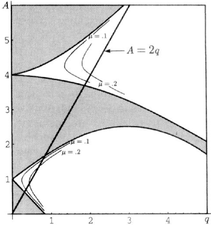
Figure 2.1: Sketch of the stability/instability chart of the canonical Mathieu equation [30].

This process of particle production due to parametric resonance of the field is called preheating. It should still be said this is not necessary for particle production to occur. Indeed, if $\xi=0$, which is the standard reheating regime, there still is a parametric oscillation with $q=0$ due to the expansion of the Universe alone. Nonetheless, the preheating scenario is much more efficient than standard reheating.

2.3 Solar System Effect

Even though $f(R)$ gravity might explain the accelerated expansion of the Universe in the inflation and present eras, its validity at the Solar System scale should be assessed. The long-range impact of $f(R)$ in the Solar System is taken into account by considering the flat FLRW metric with a spherically symmetric perturbation

$$ds^{2}=-\left[1+2\Psi(r)\right]dt^{2}+a(t)^{2}\left(\left[1+2\Phi(r)\right]dr^{2}+r^{2}d\Omega^{2}\right),$$ (2.36)

where $\Psi$ and $\Phi$ are perturbing functions such that $\left|\Psi(r)\right|\ll 1$ and $\left|\Phi(r)\right|\ll 1$.

The background curvature is nonzero, $R_{0}(t)\neq 0$, thus it can be decomposed into a sum of two components:

$$R(r,t)\equiv R_{0}(t)+R_{1}(r),$$ (2.37)

where $R_{1}(r)$ is considered as a time-independent perturbation of the background curvature. This analysis follows the work of Ref. [31]. The validity of the following treatment assumes that $R_{1}\ll R_{0}$.

The background curvature solves the trace of the field equations (2.4) according to

$$f_{R0}(t)R_{0}(t)-2f_{0}(t)+3\square f_{R0}(t)=T^{\text{cos}}(t),$$ (2.38)

where $f_{R0}\equiv df/dR\big{|}_{R=R_{0}}$, $f_{0}\equiv f(R_{0})$ and $T^{\text{cos}}$ is the trace of the energy-momentum tensor of cosmological baryonic matter.

Considering that all derivatives of $f(R)$ are well defined at $R_{0}(t_{0})$, where $t_{0}$ is the present time, a Taylor expansion around $R_{0}$ can be used to write the functions $f(R_{0}+R_{1})$ and $f_{R}(R_{0}+R_{1})$. As the framework is a weak-field regime, the expansion neglects terms non-linear in the perturbation $R_{1}$, provided that the following conditions are taken into account:

$$f_{0}+f_{R0}R_{1} \gg \dfrac{1}{n!}f^{(n)}(R_{0})R^{n}_{1},$$

$$f_{R0}+f_{RR0}R_{1} \gg \dfrac{1}{n!}f^{(n+1)}(R_{0})R^{n}_{1}\text{ for all }n>1,$$ (2.39)

where $f_{RR0}\equiv d^{2}f/dR^{2}\big{|}_{R=R_{0}}$ and $f^{(n)}(R_{0})=d^{n}f/dR^{n}\big{|}_{R=R_{0}}$.

Applying these expansions into the complete trace equation

$$f_{R}R-2f+3\square f_{R}=T^{\text{cos}}+T^{\text{s}},$$ (2.40)

where $T^{\text{s}}$ is the energy-momentum tensor of a spherically symmetric mass source, the trace equation becomes linearized as

$$3f_{RR0}\square R_{1}(r)-\left[f_{R0}(t)-f_{RR0}(t)R_{0}(t)-3\square f_{RR0}(t)\right]R_{1}=T^{\text{s}},$$ (2.41)

where equation (2.38) was used to eliminate all the terms independent of $R_{1}$. It is worthy of note that this linearization is taking into account the already stated condition $R_{1}\ll R_{0}\neq 0$, due to the presence of the term $f_{RR0}R_{0}R_{1}$, while neglecting terms of the order $f_{RR0}R_{1}^{2}$.

Since $R_{1}(r)$ is time-independent, the operator $\square$ becomes $\square\approx\nabla^{2}$. The matter at the local perturbation will be considered with no pressure, such that $T^{\text{s}}=-\rho(r)c^{2}$. Therefore, the equation (2.41) can be written as

$$\nabla^{2}R_{1}-m^{2}R_{1}=-\dfrac{\rho}{3f_{RR0}},$$ (2.42)

with

$$m^{2}\equiv\frac{1}{3}\left(\frac{f_{R0}}{f_{RR0}}-R_{0}-3\frac{\square f_{RR0}}{f_{RR0}}\right).$$ (2.43)

This equation can be solved by means of the Green function

$$G(r)=\left\{\begin{array}[]{l l}-\cos(mr)/(4\pi r)&\quad\text{if }m^{2}<0\\ \\ -\exp(-mr)/(4\pi r)&\quad\text{if }m^{2}>0\end{array}\right..$$ (2.44)

2.3.1 Long Range Regime

Considering first the long range regime $mr\ll 1$, both parts of the Green function can be approximated by $-1/(4\pi r)$. This means that the term linear in $R_{1}$ from (2.42) may disappear and the solution for the curvature perturbation becomes

$$R_{1}=\dfrac{1}{12\pi f_{RR0}}\dfrac{M_{S}}{r},$$ (2.45)

where $M_{S}$ is the total mass of the solar-like source.

Adopting the arguments for linearization from (2.39), using the background curvature equation (2.41) and neglecting all the terms that are not linear in $R_{1}$, $\Phi$ and $\Psi$, the solutions for these perturbations are taken from the time ($tt$) and radial ($rr$) components of the field equations.

The linearization of the $tt$ component of (2.2) has the form

$$f_{R0}\nabla^{2}\Psi+\dfrac{1}{2}f_{R0}R_{1}-f_{RR0}\nabla^{2}R_{1}=\rho.$$ (2.46)

Importing equation (2.42) with $m^{2}=0$ reduces the above to

$$f_{R0}\nabla^{2}\Psi=\dfrac{2}{3}\rho-\dfrac{1}{2}f_{R0}R_{1},$$ (2.47)

which can be decomposed according to $\Psi=\Psi_{0}+\Psi_{1}$, where

$$f_{R0}\nabla^{2}\Psi_{0} = \dfrac{2}{3}\rho,$$ (2.48)

$$f_{R0}\nabla^{2}\Psi_{1} = -\dfrac{1}{2}f_{R0}R_{1}.$$ (2.49)

The first of these is integrated with Gauss’s Theorem and becomes

$$\Psi_{0}^{\prime}(r)=\dfrac{1}{6\pi f_{R0}}\dfrac{m(r)}{r^{2}},$$ (2.50)

where the prime represents differentiation with respect to $r$ and $m(r)$ is the mass of a sphere with radius $r$. Assuming that $\lim_{r\to\infty}\Psi_{0}=0$, the solution for $\Psi_{0}$ is

$$\Psi_{0}=-\dfrac{1}{6\pi f_{R0}}\dfrac{M_{S}}{r}.$$ (2.51)

One the other hand, using the solution for $R_{1}$ from (2.45) in (2.49) and integrating it outside the star, gives

$$\left|\Psi_{1}\right|=\dfrac{1}{48\pi f_{RR0}}M_{S}r.$$ (2.52)

To treat this equation it is relevant to expand the condition $mr\ll 1$ with the definition of $m$, presented after Eq. (2.42):

$$\begin{split}\left|m^{2}\right|r^{2}\equiv\left|\dfrac{1}{3}\left(\dfrac{f_{R0}}{f_{RR0}}-R_{0}-3\dfrac{\square f_{RR0}}{f_{RR0}}\right)\right|r^{2}&\ll 1\\ \Rightarrow\left|\dfrac{f_{R0}}{f_{RR0}}\right|r^{2}-\left|R_{0}-3\dfrac{\square f_{RR0}}{f_{RR0}}\right|r^{2}&\ll 1,\end{split}$$ (2.53)

where the triangle inequality was used. Taking into account that $\square f_{RR0}/f_{RR0}\sim H^{2}$ and knowing by cosmological constraints that $R_{0}r^{2}\sim H_{0}^{2}r_{0}^{2}\ll 1$, then the constraint $mr\ll 1$ can be written as

$$\left|\dfrac{f_{R0}}{f_{RR0}}\right|r^{2}\ll 1.$$ (2.54)

This allows to write the useful condition $|\Psi_{1}|\sim M_{S}r/f_{RR0}\ll M_{S}/(f_{R0}r)$. Since $\Psi_{0}\sim M_{S}/(f_{R0}r)$ implies the condition $\left|\Psi_{1}\right|\ll\left|\Psi_{0}\right|$, then $\Psi_{1}$ may be neglected, thus $\Psi\equiv\Psi_{0}$.

Following the same procedures, the linearization of the $rr$ component of (2.2) takes the form

$$f_{R0}\left(-\Psi^{\prime\prime}+\dfrac{2}{r}\Phi^{\prime}\right)-\dfrac{1}{2}f_{R0}R_{1}+\dfrac{2}{r}f_{RR0}R_{1}^{\prime}=0.$$ (2.55)

First of all, the second term of the equation can be neglected with respect to the last one, due to the application of (2.54) as

$$\left|\dfrac{(1/2)f_{R0}R_{1}}{2f_{RR0}R_{1}^{\prime}/r}\right|\sim\left|\dfrac{f_{R0}}{f_{RR0}}\right|r^{2}\ll 1.$$ (2.56)

Computing $\Psi^{\prime\prime}$ from (2.50) and $R_{1}^{\prime}$ from (2.42) (with $m^{2}=0$), Eq. (2.55) can be written as

$$\Phi^{\prime}(r)=\dfrac{1}{12\pi f_{R0}}\dfrac{d}{dr}\left[\dfrac{m(r)}{r}\right],$$ (2.57)

which can be integrated outside the matter source and with the outer limit $\lim_{r\to\infty}\Phi=0$ to give

$$\Phi=\dfrac{1}{12\pi f_{R0}}\dfrac{M_{S}}{r}.$$ (2.58)

Comparing the solution $\Phi$ with $\Psi$, from (2.48), it is easy to conclude that $\Psi=-2\Phi$, thus implying that the Parametrized Post-Newtonian (PPN) parameter $\gamma=-\Phi/\Psi$ takes the value $\gamma=1/2$, which contradicts the observational results that yield $\gamma\sim 1$ [2] — implying that, if the additional degree of freedom is long-ranged ($mr\ll 1$), $f(R)$ gravity is incompatible with experiment. Notice that, in BD theories, $\gamma=1/2$ is obtained from $\omega=0$: following the discussion after Eq. (2.10), the very light mass implies that the potential has no impact on the dynamics, and as such this result only restates that an $f(R)$ model with this characteristic is observationally excluded.

2.3.2 Short Range Regime

To obtain a valid $f(R)$ model one should then study the case where the spherical symmetric mass is sufficiently big to make an impact, ie the short range regime of $f(R)$ should be studied. And, to study the short range regime of $f(R)$ gravity in the Solar System, it is more adequate to consider a perturbation of a Minkowski metric of the form

$$ds^{2}=-\left[1+2\Psi\left(r\right)\right]c^{2}dt^{2}+\left[1+2\Phi(r)\right]dr^{2}+r^{2}d\Omega^{2},$$ (2.59)

where $\Psi$ and $\Phi$ are again perturbing functions such that $\left|\Psi(r)\right|\ll 1$ and $\left|\Phi(r)\right|\ll 1$. This is so because if $f(R)$ is short-ranged ($mr\gg 1$), the dynamics of the Universe do not have any impact at Solar System scales, while in the opposite case (long range, $mr\ll 1$), the effect of $f(R)$ extends to much longer distances, so that the asymptotic values of cosmology must be taken into account.

In the following it is assumed that matter behaves as dust, $i.e.$ a perfect fluid with negligible pressure and an energy-momentum tensor described by

$$T_{\mu\nu}=\rho c^{2}u_{\mu}u_{\nu}\leavevmode\nobreak\ \leavevmode\nobreak\ \leavevmode\nobreak\ \leavevmode\nobreak\ ,\leavevmode\nobreak\ \leavevmode\nobreak\ \leavevmode\nobreak\ \leavevmode\nobreak\ u_{\mu}u^{\mu}=-1,$$ (2.60)

where $\rho$ is the matter density and $u_{\mu}$ is the four-velocity vector. The same procedure was followed in the long-range situation, though it was not as detailed as in this section. The trace of the energy-momentum tensor is $T=-\rho c^{2}$. The Lagrangian density of matter is considered as ${\cal L}_{m}=-\rho c^{2}$ (see Ref. [32] for a discussion).

The function $\rho=\rho(r)$ is that of a spherically symmetric body with a static radial mass density $\rho=\rho(r)$ and the function $\rho(r)$ and its first derivative are assumed to be continuous across the surface of the body,

$$\rho(R_{S})=0\quad\text{and}\quad\dfrac{d\rho}{dr}(R_{S})=0,$$ (2.61)

where $R_{S}$ denotes the radius of the spherical body. These conditions play a role in the following sections, where integrals that have $R_{S}$ as an integration limit appear.

This analytical setup allows to define the function $f(R)$ as a Taylor expansion around $R=0$, according to Ref. [33]:

$$f(R)\approx 2\kappa\left(R+\dfrac{R^{2}}{6m^{2}}\right)+{\cal O}(R^{3}),$$ (2.62)

which is similar to the Starobinsky action functional from (2.13), although here the mass $m$ is related to the second derivative of the more general $f(R)$ function, while in the latter this was considered to be exact.

Repeating what was done in the long range regime, the equations for the curvature and for the perturbations $\Psi$ and $\Phi$ will be linearized. In this case, the linearization is done according to the expansion of each of these three quantities in powers of $c^{-1}$ and all the terms of the order ${\cal O}(c^{-3})$ or less are neglected.

Inserting (2.62) into the curvature equation (2.4) and linearizing it, yields

$$\nabla^{2}R-m^{2}R=-\dfrac{8\pi G}{c^{2}}m^{2}\rho,$$ (2.63)

which through the variable substitution $u=rR$ becomes

$$\dfrac{d^{2}u}{dr^{2}}-m^{2}u=s(r),$$ (2.64)

where $s(r)=-\left(8\pi G/c^{2}\right)m^{2}r\rho$ is the source function. The function $u(r)$ respects the following boundary conditions:

• $u(0)=0$, so that the curvature $R$ may have a finite value at that point;

• $\lim_{r\to\infty}u(r)=0$, so that the curvature vanishes asymptotically as one recovers the Minkowski metric.

The Green function of (2.64) in the sense of distributions solves the equation

$$\dfrac{d^{2}G(r,r^{\prime})}{dr^{\prime 2}}-m^{2}G(r,r^{\prime})=\delta(r-r^{\prime}),$$ (2.65)

where $\delta(r-r^{\prime})$ is a Dirac delta distribution. This Green function $G(r,r^{\prime})$ is used to determine the solution of the curvature equation by means of the integral $u(r)=\int^{r}_{0}G(r,r^{\prime})s(r^{\prime})dr^{\prime}$. Due to the different boundary conditions, the curvature is written as a twofold solution:

$$R(r)=\left\{\begin{array}[]{l l}R^{\uparrow}(r)&\quad\text{if }r>R_{S}\\ \\ R^{\downarrow}(r)&\quad\text{if }0\leq r\leq R_{S}\end{array}\right.,$$ (2.66)

where $R^{\downarrow}(r)$ is the curvature inside the star

$$R^{\downarrow}(r)=-\dfrac{4\pi G}{c^{2}m}\left[\dfrac{e^{-mr}}{r}I_{1}(r)+\dfrac{2\sinh(mr)}{r}I_{2}(r)\right].$$ (2.67)

The quantities $I_{1}(r)$ and $I_{2}(r)$ have been computed by using the properties (2.61) of the mass density $\rho(r)$ and are given by

$$I_{1}(r) = -2m^{2}\int^{r}_{0}\sinh(mr^{\prime})r^{\prime}\rho(r^{\prime})dr^{\prime},$$

$$I_{2}(r) = -m^{2}\int^{R_{S}}_{r}e^{-mr^{\prime}}r^{\prime}\rho(r^{\prime})dr^{\prime}.$$

On the other hand, $R^{\uparrow}(r)$ is the curvature outside the star, given by

$$R^{\uparrow}(r)=\dfrac{2GM_{S}}{rc^{2}}m^{2}A(m,R_{S})e^{-mr},$$ (2.68)

where $A(m,R_{S})$ is a form factor defined as

$$A(m,R_{S})=\dfrac{4\pi}{mM_{S}}\int^{R_{S}}_{0}\sinh(mr)r\rho(r)dr,$$ (2.69)

which shall be discussed in a subsequent section.

As for the solution of $\Psi$, it is obtained through the linearization of the $tt$ component of the field equations (2.2), neglecting all terms smaller than ${\cal O}(1/c^{2})$, combined with the $tt$ component of the Ricci tensor at order ${\cal O}(1/c^{2})$,

$$R_{tt}=\dfrac{2\Psi^{\prime}}{r}+\Psi^{\prime\prime}+{\cal O}\left(\dfrac{1}{c^{3}}\right)=\nabla^{2}\Psi+{\cal O}\left(\dfrac{1}{c^{3}}\right),$$ (2.70)

while the curvature equation (2.63) yields the expression ruling $\Psi$:

$$\nabla^{2}\Psi=\dfrac{c^{2}}{3k}\rho-\dfrac{R}{6}.$$ (2.71)

This is solved outside the spherical body, $r\geq R_{S}$, by decomposing it into a sum,

$$\nabla^{2}\Psi=\nabla^{2}\Psi_{0}+\nabla^{2}\Psi_{1},$$ (2.72)

where

$$\nabla^{2}\Psi_{0}=\dfrac{c^{2}}{3k}\rho\leavevmode\nobreak\ \leavevmode\nobreak\ \leavevmode\nobreak\ \leavevmode\nobreak\ ,\leavevmode\nobreak\ \leavevmode\nobreak\ \leavevmode\nobreak\ \leavevmode\nobreak\ \nabla^{2}\Psi_{1}=-\dfrac{R}{6}.$$ (2.73)

The first equation is easily solved using the divergence theorem, which gives

$$\Psi_{0}(r)=-\dfrac{4}{3}\dfrac{GM_{S}}{c^{2}r}.$$ (2.74)

The second one needs a longer integration, which eventually shows that

$$\Psi_{1}(r)=\dfrac{GM_{S}}{3c^{2}r}\left[1-A(m,R_{S})e^{-mr}\right],$$ (2.75)

so that for $r\geq R_{S}$ the solution is

$$\Psi(r)=-\dfrac{GM_{S}}{c^{2}r}\left[1+\dfrac{1}{3}A(m,R_{S})e^{-mr}\right].$$ (2.76)

Taking the $rr$ component of the Ricci tensor to the usual order of ${\cal O}(1/c^{2})$ and recording that the mass distribution is static yields

$$R_{rr}=\dfrac{2}{r}\Phi^{\prime}-\Psi^{\prime\prime}+{\cal O}\left(\dfrac{1}{c^{3}}\right)\leavevmode\nobreak\ \leavevmode\nobreak\ \leavevmode\nobreak\ \leavevmode\nobreak\ ,\leavevmode\nobreak\ \leavevmode\nobreak\ \leavevmode\nobreak\ \leavevmode\nobreak\ T_{rr}=0,$$ (2.77)

so that the $rr$ component of the field equations (2.2) becomes

$$2\Phi^{\prime}-r\Psi^{\prime\prime}-\dfrac{rR}{2}+\dfrac{2R^{\prime}}{3m^{2}}=0.$$ (2.78)

This equation is easily integrated outside the spherical body, $r\geq R_{S}$, leading to

$$\Phi(r)=\dfrac{GM_{S}}{c^{2}r}\left[1-\dfrac{1}{3}A(m,R_{S})e^{-mr}(1+mr)\right].$$ (2.79)

In the GR limit, $m\to\infty$, the exponential term in both $\Psi$ and $\Phi$ vanishes and the weak-field approximation of the Schwarzschild metric is obtained, as expected from a weak spherical perturbation on a Minkowski metric.

It should be noted that if the metric (2.59) is written in the isotropic coordinates

$$ds^{2}=-\left[1+2\Psi^{\prime}(r^{\prime})\right]dt^{\prime 2}+\left[1+2\Phi^{\prime}(r^{\prime})\right]\left(dr^{\prime 2}+r^{\prime 2}d\Omega^{\prime 2}\right],$$ (2.80)

then the perturbing functions (5.19) and (5.22) become

$$\Psi^{\prime}(r^{\prime}) = -\dfrac{GM_{S}}{c^{2}r^{\prime}}\left[1+\dfrac{1}{3}A(m,R_{S})e^{-mr}\right],$$ (2.81)

$$\Phi^{\prime}(r^{\prime}) = \dfrac{GM_{S}}{c^{2}r^{\prime}}\left[1-\dfrac{1}{3}A(m,R_{S})e^{-mr}\right],$$ (2.82)

which differ only in the signal of the second term.

These results should not be analysed with the PPN formalism, as they instead depict a Yukawa type correction to the Newtonian potential with a field strength $1/3$. This kind of Yukawa correction to the Newtonian potential is not new in physics and many experimental tests have been made on it, as shall be discussed in a subsequent chapter.

Chapter 3 Nonminimal Coupling

The remarkable range of applications of $f(R)$ gravity, and in particular the Starobinsky inflationary model, prompted physicists to generalize these theories even further. This generalization is made by a nonminimal coupling (NMC) between geometry and matter, through the product of the matter Lagrangian density with another function of the curvature, as posited by the action [34]

$$S_{\text{NMC}}=\int\left[\dfrac{1}{2}f^{1}(R)+\left[1+f^{2}(R)\right]{\cal L}_{m}\right]\sqrt{-g}d^{4}x.$$ (3.1)

The field equations, obtained through the variation of the action with respect to the metric, are

$$\left(f^{1}_{R}+2f^{2}_{R}{\cal L}_{m}\right)R_{\mu\nu}-\dfrac{1}{2}f^{1}g_{\mu\nu}=\left(1+f^{2}\right)T_{\mu\nu}+\left(\square_{\mu\nu}-g_{\mu\nu}\square\right)\left(f^{1}_{R}+2f^{2}_{R}{\cal L}_{m}\right),$$ (3.2)

where $f_{R}^{i}\equiv df^{i}(R)/dR$. If $f^{1}(R)=2\kappa(R-2\Lambda)$ and $f^{2}(R)=0$, then the action (3.1) collapses to the Einstein-Hilbert action from (1.1). The Palatini formulation of a NMC theory, obtained by considering that the metric and affine connection are a priori independent, can be found in Ref. [35].

It should be said that, in opposition to GR and pure $f(R)$ gravity, these field equations do not respect the conservation of energy law, $\nabla^{\mu}T_{\mu\nu}\neq 0$. Indeed, the covariant derivative of the field equations (3.2), together with the Bianchi identities $\nabla^{\mu}G_{\mu\nu}=0$ and the identity

$$(\square\nabla_{\nu}-\nabla_{\nu}\square)f_{R}^{i}=R_{\mu\nu}\nabla^{\mu}f_{R}^{i},$$ (3.3)

yields for the covariant derivative of the energy-momentum tensor,

$$\nabla^{\mu}T_{\mu\nu}=\dfrac{f_{R}^{2}}{1+f^{2}}\left(g_{\mu\nu}{\cal L}_{m}-T_{\mu\nu}\right)\nabla^{\mu}R.$$ (3.4)

Nonetheless, if $f^{2}(R)=0$, the pure $f(R)$ case is recovered and the conservation law is fulfilled. This non-conservation of the energy-momentum tensor may yield a violation of the Equivalence principle, for the nonminimal coupling between geometry and matter means that the motion of matter is dependent on the specific form of the Lagrangian density ${\cal L}_{m}$ and thus matter may not follow the expected geodesic motion.

It should also be mentioned that NMC has an impact on the description of the interior of a central body, leading to a correction to the latter’s coupling strength, as is illustrated in Refs. [36, 37, 38].

3.1 Scalar-fields equivalence

In section 2.1, the pure $f(R)$ gravity theories were shown to be equivalent to scalar-tensor theories $-$ in particular, to a BD theory of gravity. NMC theories of gravity can also be written in a similar way, though with two independent scalar fields [39]. These theories are introduced through the action

$$S=\int\left[\dfrac{1}{2}f^{1}(\phi)+\left[1+f^{2}(\phi)\right]{\cal L}_{m}+\psi(R-\phi)\right]\sqrt{-g}d^{4}x,$$ (3.5)

where $\psi$ acts as a Lagrange multiplier imposing the relation $\phi=R$, with which the action $S$ is reduced to $S_{NMC}$. The variation of this action (3.5) with respect to $\phi$ then yields

$$\psi=\dfrac{1}{2}f^{1}_{R}(\phi)+f_{R}^{2}(\phi){\cal L}_{m},$$ (3.6)

which indicates that both scalar-fields are independent if ${\cal L}_{m}\neq 0$ or $f_{R}^{2}\neq 0$. If $f_{R}^{2}=0$, then the action returns to the pure $f(R)$ case.

As in the pure $f(R)$ situation, the action (3.5) can be written in the form of a BD theory with $\omega_{BD}=0$ (check Eq. (2.10)) and the same scalar-fields,

$$S=\int\left[\psi R-V(\phi,\psi)+\left[1+f^{2}(\phi)\right]{\cal L}_{m}\right]\sqrt{-g}d^{4}x,$$ (3.7)

with the potential

$$V(\phi,\psi)=\phi\psi-\dfrac{1}{2}f^{1}(\phi).$$ (3.8)

3.2 Preheating and Inflation

In section 2.2.1, the process of particle production after inflation was explained by means of a preheating mechanism, whose main characteristic was on the parametric resonance of a quantum field $\chi$. The action of this field included a NMC term between the curvature and the field itself, of the type $\xi R\chi^{2}$ $-$ i.e. an additional mass term. This linear NMC prompts for the more general assumption of the action (3.1) with the functions

$$f^{1}(R)=2\kappa\left(R+\dfrac{R^{2}}{6M^{2}}\right),\leavevmode\nobreak\ \leavevmode\nobreak\ \leavevmode\nobreak\ \qquad\qquad\leavevmode\nobreak\ \leavevmode\nobreak\ \leavevmode\nobreak\ \leavevmode\nobreak\ \leavevmode\nobreak\ \leavevmode\nobreak\ f^{2}(R)=2\xi\dfrac{R}{M^{2}}.$$ (3.9)

Logically, this specific action has to be able to explain inflation at the standard SRA, which means that $f^{2}(R)$ should interfere only in the preheating situation, and so the NMC model only works as part of a perturbative regime with $f^{2}(R)\sim 0$.

As stated in section 2.2, the mass parameter has the value $M\sim 10^{13}$ GeV$/c^{2}$, whereas the NMC parameter $\xi$ is dimensionless and subject to the range $1<\xi<10^{4}$. The lower bound $\xi>1$ was established in order to provide the validity of the condition $R\gg M^{2}/(2\xi)$ throughout the SRA regime. The upper bound of $\xi<10^{4}$ is obtained by resorting to the initial inflationary temperature [40].

As in Eq. (2.29), the decomposition of the scalar field from the NMC in Fourier modes yields that each mode is governed by

$$\ddot{\chi}_{k}+\left(3H+\dfrac{f^{2}_{R}}{\left(1+f^{2}\right)}\dot{R}\right)\dot{\chi}_{k}+\left(\dfrac{k^{2}}{a^{2}}+m^{2}\right)\chi_{k}=0.$$ (3.10)

The redefinition $X_{k}\equiv a^{3/2}\sqrt{f^{2}}\chi_{k}$ and the new variable $z$ defined by $2z=M\left(t-t_{0}\right)\pm\pi/2$ (depending on the sign of $\xi$) allows to transform the previous equation into

$$X_{k}^{\prime\prime}+\left[\left(\dfrac{2k}{aM}\right)^{2}+\left(\dfrac{2m}{M}\right)^{2}-3\dfrac{H^{\prime}}{M}-9\dfrac{H^{2}}{M^{2}}+\dfrac{1}{2}\dfrac{f_{R}^{2}}{\left(1+f^{2}\right)}\left(\dfrac{1}{2}\dfrac{f_{R}^{2}}{\left(1+f^{2}\right)}R^{\prime 2}-6\dfrac{HR^{\prime}}{M}-R^{\prime\prime}\right)\right]X_{k}=0,$$ (3.11)

where the prime represents a derivative with respect to $z$. Recalling that this action is valid in a $f^{2}(R)\approx 0$ regime, the above equation can be expanded as,

$$X_{k}^{\prime\prime}+\left[\left(\dfrac{2k}{aM}\right)^{2}+\left(\dfrac{2m}{M}\right)^{2}-3\dfrac{H^{\prime}}{M}-9\dfrac{H^{2}}{M^{2}}++\dfrac{\xi}{M^{2}}\left(\xi\dfrac{R^{\prime 2}}{M^{2}}-6\dfrac{HR^{\prime}}{M}-R^{\prime\prime}\right)\right]X_{k}=0.$$ (3.12)

As discussed before, the fact that after the SRA the parameter $z$ answers to the late-time approximation $z\gg 1$ makes the Hubble parameter and curvature go through an oscillatory phase of the type

$$H(z)\simeq\dfrac{M}{3z}\left[1+\sin(2z)\right],\qquad\qquad\qquad R(z)\simeq 3MH^{\prime}(z)\simeq\dfrac{2M^{2}}{z}\cos(2z).$$ (3.13)

This is the path to show that $R^{\prime\prime}$ term dominates [40], so the equation of $X_{k}$ can be written as

$$X_{k}^{\prime\prime}+\left[\left(\dfrac{2k}{aM}\right)^{2}+\left(\dfrac{2m}{M}\right)^{2}-\xi\dfrac{R^{\prime\prime}}{M^{2}}\right]X_{k}=0,$$ (3.14)

which may be written in the form of the Mathieu equation

$$X_{k}^{\prime\prime}+\left[A_{k}-2q\cos(2z)\right]X_{k}=0,\qquad\qquad A_{k}=\left(\dfrac{2k}{aM}\right)^{2}+\left(\dfrac{2m}{M}\right)^{2},\qquad\qquad q=\dfrac{4\xi}{z}.$$ (3.15)

The interesting fact is that with a NMC term in the action, the resulting equation is the same as the one obtained in (2.34). The results are, therefore, identical to the ones mentioned in section 2.2.1.

3.3 Solar System Long Range Regime

Moving forward the parallelism with the pure $f(R)$ case from chapter 2, the NMC impact at the Solar System scales is analysed. As in section 2.3, matter is assumed to behave as dust, described by Eq. (2.60), so that the trace of the energy-momentum tensor is $T=-\rho c^{2}$ and the Lagrangian density of matter is treated as ${\cal L}_{m}=-\rho c^{2}$.

The function $\rho=\rho(r)$ is again that of a spherically symmetric body with a static radial mass density $\rho=\rho(r)$. This function $\rho(r)$ and its first derivative are assumed to obey Eqs. (2.61).

The metric used is once more the perturbed FLRW metric, repeated here for convenience:

$$ds^{2}=-\left[1+2\Psi(r)\right]dt^{2}+a(t)^{2}\left(\left[1+2\Phi(r)\right]dr^{2}+r^{2}d\Omega^{2}\right),$$ (3.16)

where $\Psi$ and $\Phi$ are perturbing functions such that $\left|\Psi(r)\right|\ll 1$ and $\left|\Phi(r)\right|\ll 1$. The scalar curvature of this spacetime is also expressed as the sum of a time evolving cosmological contribution $R_{0}(t)$ and a perturbation $R_{1}(r)$, induced by the local matter distribution,

$$R(r,t)\equiv R_{0}(t)+R_{1}(r),\leavevmode\nobreak\ \leavevmode\nobreak\ \leavevmode\nobreak\ \leavevmode\nobreak\ \qquad\leavevmode\nobreak\ \leavevmode\nobreak\ \leavevmode\nobreak\ \leavevmode\nobreak\ \left|R_{1}(r)\right|\ll R_{0}(t).$$ (3.17)

This assumption allows to expand the functions $f^{i}(R)$ around $R=R_{0}$ and neglect all the nonlinear terms in $R_{1}$. This approximation is the same as the one detailed in Eq. (2.39), with the exception that now both $f^{1}(R)$ and $f^{2}(R)$ are subject to it.

3.3.1 Solution for the curvature $R_{1}$

The trace of the field equations (3.2) is

$$\left(f^{1}_{R}+2f^{2}_{R}{\cal L}_{m}\right)R-2f^{1}=-3\square\left(f^{1}_{R}+2f^{2}_{R}{\cal L}_{m}\right)+\left(1+f^{2}\right)T.$$ (3.18)

Considering the decomposition of the energy-momentum tensor as $T_{\mu\nu}=T^{\text{cos}}_{\mu\nu}+T^{\text{s}}_{\mu\nu}$ and of the matter density as $\rho=\rho^{\text{cos}}(t)+\rho^{\text{s}}(r)$, the trace equation for the background curvature has the following solution

$$\left(f^{1}_{R0}+2f^{2}_{R0}{\cal L}^{\text{cos}}_{m}\right)R_{0}-2f_{0}^{1}+3\square\left(f^{1}_{R0}+2f^{2}_{R0}{\cal L}^{\text{cos}}_{m}\right)=\left(1+f^{2}_{0}\right)T^{\text{cos}}.$$ (3.19)

Inserting this equation into (3.18) and taking into account that all terms of order ${\cal O}(R_{1}^{2})$ or greater are neglected, yields

$$\begin{split}\left[-f^{1}_{R0}+f^{2}_{R0}{\cal L}_{m}+\left(f^{1}_{RR0}+2f^{2}_{RR0}{\cal L}_{m}\right)R_{0}\right]R_{1}+&3\square\left[\left(f^{1}_{RR0}+2f^{2}_{RR0}{\cal L}_{m}\right)R_{1}\right]=\\ &\left(1+f^{2}_{0}\right)T^{\rm s}-2f^{2}_{R0}{\cal L}_{m}^{\rm s}R_{0}-6\square\left(f^{2}_{R0}{\cal L}_{m}^{\rm s}\right).\end{split}$$ (3.20)

The expansion of the operator $\square$ and neglecting products of $R_{1}$ or of its spatial derivatives with $\Psi$ and $\Phi$ and their spatial derivatives, gives the curvature equation the expression

$$\nabla^{2}U-m^{2}U=-\frac{1}{3}\left(1+f^{2}_{0}\right)\rho^{\rm s}+\frac{2}{3}f^{2}_{R0}\rho^{\rm s}R_{0}+2\rho^{\rm s}\square f^{2}_{R0}+2f^{2}_{R0}\nabla^{2}\rho^{\rm s},$$ (3.21)

where the potential $U(r,t)$ is defined as

$$U(r,t)=\left[f^{1}_{RR0}(t)+2f^{2}_{RR0}(t){\cal L}_{m}(r,t)\right]R_{1}(r),$$ (3.22)

and the mass parameter is

$$m^{2}=\frac{1}{3}\left[\frac{f^{1}_{R0}-f^{2}_{R0}{\cal L}_{m}}{f^{1}_{RR0}+2f^{2}_{RR0}{\cal L}_{m}}-R_{0}-\frac{3\square\left(f^{1}_{RR0}-2f^{2}_{RR0}\rho^{\rm cos}\right)-6\rho^{\rm s}\square f^{2}_{RR0}}{f^{1}_{RR0}+2f^{2}_{RR0}{\cal L}_{m}}\right],$$ (3.23)

where $f^{1}_{RR0}+2f^{2}_{RR0}{\cal L}_{m}\neq 0$ is assumed. Naturally, this expression becomes the one obtained for the pure $f(R)$ theories, Eq. (2.42), when $f^{2}(R)=0$.

As a first step to work out the solution of the above equation, it is better to consider it outside the star, where $\rho^{\text{s}}=0$, so that the mass parameter depends only on time, $m=m(t)$. Equation (3.21) thus becomes

$$\nabla^{2}U=m^{2}(t)U,$$ (3.24)

and its solution is a Yukawa potential of the type

$$U\sim\dfrac{e^{-mr}}{r},$$ (3.25)

or, if $m^{2}<0$, an oscillating potential with strength $\sim 1/r$.

The condition that $m^{2}$ is positive-defined expands upon the previous stability constraint $f_{RR}^{1}+f_{RR}^{2}{\cal L}_{m}>0$ [41, 42], which is required to avoid the related Dolgov-Kawasaki instabilities [43], and can be interpreted physically as requiring that gravity is attractive; the strong, weak, null and dominant energy conditions were also addressed in Ref. [42], showing that a wide class of NMC models is allowed; in fact, a NMC allows for a minimisation of the known violation of the null energy condition in wormholes [44].

The long range regime condition $mr\ll 1$ means that $U\sim 1/r$ and so it is possible to neglect the term $m^{2}U$ in equation (3.21), when computing the total solution of $U(r,t)$. It follows then that equation (3.21) becomes

$$\nabla^{2}U=\eta(t)\rho^{\rm s}(r)+2f^{2}_{R0}\nabla^{2}\rho^{\rm s},$$ (3.26)

with

$$\eta(t)=-\frac{1}{3}\left(1+f^{2}_{0}\right)+\frac{2}{3}f^{2}_{R0}R_{0}+2\square f^{2}_{R0}.$$ (3.27)

Computing the solution of $U(r,t)$ outside the body, $r>R_{S}$, one obtains

$$U(r,t)=-\frac{\eta(t)}{4\pi}\frac{M_{\rm S}}{r},$$ (3.28)

where $M_{S}$ is the total mass of the spherical body. Through Eq. (3.22), the curvature $R_{1}$ is defined as

$$R_{1}(r,t)=\frac{\eta(t)}{4\pi\left(2f^{2}_{RR0}\rho^{\text{cos}}-f^{1}_{RR0}\right)}\frac{M_{\text{S}}}{r},$$ (3.29)

which obviously reduces to Eq. (2.45) when $f^{2}(R)=0$. Also, notice that the variation of $R_{1}$ in time is on a time scale much bigger than the one proper from the Solar System, so that it is plausible to assume $R_{1}(r,t)\simeq R_{1}(r)$. The $R_{1}(r)$ solution for $r<R_{S}$ is not relevant for the following analysis, so it is not presented here (for details, check Ref. [45]).

3.3.2 Solution for $\Psi$ and $\Phi$

The same linearization procedure that was used for the curvature may be used for the $tt$ and $rr$ components of the field equations (3.2). The computation of $\Psi$ once more goes through a decomposition of the type $\Psi=\Psi_{0}+\Psi_{1}$ and the computation of $\Phi$ is nothing more than a simple integration. The development of these computations is beyond the scope of this section analysis, whose main point is simply to present the results of the long range Solar System effect of the NMC. Nonetheless, for more details one should resort to Ref. [45].

The final solution for $\Psi$ outside the spherical body is,

$$\Psi(r,t)=-\frac{1+f^{2}_{0}+f^{2}_{R0}R_{0}+3\square f^{2}_{R0}}{6\pi\left(f^{1}_{R0}-2f^{2}_{R0}\rho^{\rm cos}\right)}\,\frac{M_{S}}{r},\qquad r\geq R_{S},$$ (3.30)

which, if $f^{2}(R)=0$, is reduced to the solution of $\Psi$ from section 2.3.1. This expression can be said to include a gravitational coupling slowly varying in time,

$$G_{\text{eff}} = \frac{\omega(t)}{6\pi\left(f^{1}_{R0}-2f^{2}_{R0}\rho^{\rm cos}\right)},$$ (3.31)

$$\omega(t) = 1+f^{2}_{0}+f^{2}_{R0}R_{0}+3\square f^{2}_{R0}.$$

This expression shows that the timescale $\dot{G}_{\text{eff}}/G_{\text{eff}}$ is much bigger than the timescale of the Solar System, and thus the approximations $G_{\text{eff}}\simeq{\rm const.}$ and $\Psi(r,t)\simeq\Psi(r)$ can be made. The available bounds on $\dot{G}_{\text{eff}}/G_{\text{eff}}$ [46] may help to constrain $f^{1}(R)$ and $f^{2}(R)$ through Eq. (3.31). The Newtonian limit also requires that $\Psi(r)$ should be proportional to $M_{S}/r$, leading to the following constraint on the functions $f^{1}(R)$ and $f^{2}(R)$:

$$\left|2f^{2}_{R0}\right|\rho^{\text{s}}(r)\ll\left|f^{1}_{R0}-2f^{2}_{R0}\rho^{\text{cos}}(t)\right|,\qquad r\leq R_{S}.$$ (3.32)

On the other hand, together with the obtained solutions of $R_{1}$ and $\Psi$, the $rr$ component of the field equations yields for $\Phi$ the solution

$$\Phi(r,t)=\frac{1+f^{2}_{0}+4f^{2}_{R0}R_{0}+12\square f^{2}_{R0}}{12\pi\left(f^{1}_{R0}-2f^{2}_{R0}\rho^{\rm cos}\right)}\,\frac{M_{\rm S}}{r},$$ (3.33)

where $\Phi(r,t)\simeq\Phi(r)$ is once more valid. When $f^{2}(R)=0$, the solution for $\Phi$ becomes the one from the pure $f(R)$ gravity, (2.58).

Having the solutions of both potentials $\Psi$ and $\Phi$, the PPN parameter $\gamma$ is then

$$\gamma=\frac{1}{2}\,\left[\frac{1+f^{2}_{0}+4f^{2}_{R0}R_{0}+12\square f^{2}_{R0}}{1+f^{2}_{0}+f^{2}_{R0}R_{0}+3\square f^{2}_{R0}}\right],$$ (3.34)

showing that it is completely defined by the background metric $R_{0}$, whose value is obtained from the cosmological solution of NMC gravity, developed in Ref. [47]. The case $f^{2}(R)=0$ obviously yields the value $\gamma=1/2$ from the computations of section 2.3.1. However, it should be said that this expression for $\gamma$ does not work properly when the functions $f^{i}(R)$ reduce to their GR expressions, since it implies that the mass parameter $m$, defined in (3.23), is ill-defined (and divergent), so that many assumptions made to compute $\Psi$ and $\Phi$ are not satisfied [45].

Concluding the chapter, all of what was said above means that for a NMC model in a long range regime to be compatible with Solar System results, one of these conditions has to be satisfied:

• The present analysis is not adequate to test the validity of the model, because either the condition $|mr|\ll 1$ at Solar System scales shouldn’t apply or the nonlinear terms in $R_{1}$ should be considered in the Taylor expansions from (2.39) ($i.e.$ the condition $\left|R_{1}\right|\ll R_{0}$ is not satisfied);

• Or, if both conditions from point (i) are otherwise satisfied, then the validity condition of the Newtonian limit (3.32) has to be satisfied, so that the value of $\gamma$ (5.34) needs to satisfy the Cassini measurement constraint $\gamma=1+(2.1\pm 2.3)\times 10^{-5}$ [48].

To advance with condition (ii), the parameter of mass $m^{2}$ (3.23) should be computed with the cosmological solution, i.e. with the values of $R_{0}(t)$ and $\rho^{\rm cos}(t)$. For that, the functions $f^{i}(R)$ can in general assume power-law forms compatible with the description of the current phase of accelerated expansion of the Universe [47, 49], such as

$$f^{1}(R)=2\kappa R,\leavevmode\nobreak\ \leavevmode\nobreak\ \leavevmode\nobreak\ \leavevmode\nobreak\ \leavevmode\nobreak\ \qquad\leavevmode\nobreak\ \leavevmode\nobreak\ \leavevmode\nobreak\ \leavevmode\nobreak\ \leavevmode\nobreak\ f^{2}(R)=\left(\dfrac{R}{R_{n}}\right)^{-n},\leavevmode\nobreak\ \leavevmode\nobreak\ \leavevmode\nobreak\ \leavevmode\nobreak\ n>0.$$ (3.35)

The development of the conditions presented in point (i) in this power-law form of NMC gravity is detailed in Ref. [45], where the authors make the following conclusions:

• The Solar System long-range regime $|m|r\ll 1$ leads to $n\gg 10^{-25}$;

• The validity condition for the Newtonian limit (3.32) implies that $n\ll 10^{-33}$;

• The perturbative regime $\left|R_{1}\right|\ll R_{0}$ leads to an unphysical fine tuning of the density profile $\rho^{\text{s}}(r)$ inside the spherical body.

The last conclusion is related to the lack of validity of the perturbative regime and it applies to a wide range of astrophysical objects, as long as they are spherical bodies with whom the weak-field approximation can be used. This conclusion means that the procedure used, first applied in section 2.3.1, does not exclude or even constrain the NMC model. It is a null-result that nevertheless prompts to inspect more closely the inverse situation of a relevant mass parameter and a negligible cosmological background.

Chapter 4 Experimental Constraints on Modifications of GR

4.1 Tests of the Gravitational Inverse-Square Law (ISL)

The law of gravity developed by Sir Isaac Newton in the beginning of the 18${}^{\text{th}}$ century and generalized in Einstein’s GR stands as the first fundamental law of physics to be discovered (followed by electromagnetism and the weak and strong forces of quantum mechanics). Its consistency with the phenomena of nature is amazingly strong, from the small scale of a few milimeters all through to the cosmological scale. The standard gravitational ISL, originally formalized by Newton, is

$$F(r)=\dfrac{Gm_{i}m_{j}}{r^{2}},$$ (4.1)

where $G$ is Newton’s constant of gravitation and $r$ is the distance between the point masses $m_{i}$ and $m_{j}$. This expression also stems from the GR theory, in the nonrelativistic limit of weak fields.

There are, of course, some problems with the accepted GR theory of gravity, already identified in section 1.3. These are related to the need for dark matter, the present accelerated expansion of the Universe and to the compatibility of GR with quantum mechanics. Moreover, there are some phenomena arising from the solutions for this latter problem, which may be detected at the scale level of Newton’s gravitational law. These phenomena, mostly enumerated in Refs. [50, 51], are often related to forces not described in an ISL that should also account for the effects of gravity. Indeed, it is now usual to identify and constrain these deviations of the ISL through a Yukawa contribution to the potential,

$$U(r)=-G\dfrac{m_{i}}{r}\left(1+\alpha e^{-r/\lambda}\right),$$ (4.2)

where $\alpha$ is called the Yukawa strength parameter and $\lambda$ is a characteristic length scale. The motivation for this Yukawa potential comes from the presence of a massive scalar field, so that it is simply the solution of Klein-Gordon’s equation $\square\phi=m^{2}\phi$ [51], with $\lambda=1/m$. It should also be noticed that when $\lambda\to\infty$, one obtains a modification on the Newton constant $G_{N}=G\left(1+\alpha\right)$.

These parameters $\alpha$ and $\lambda$ are constrained by limits imposed from experimental results and figure 4.1 shows how large $\alpha$ can be in the different length scales dictated by $\lambda$. The overall data in this graphic is a composition from different experiments. The values of $\alpha$ above the curve, in the shaded area, are excluded as physically possible values with a $95\%$-confidence level.

Figure 4.1: Yukawa exclusion plot for $\alpha$ and $\lambda$. Adapted froms Refs. [51, 52].

The results for the left curve are determined by the torsion balance experiments from the Eöt-Wash group, presented in Ref. [53] and Refs. therein. The Keplerian and Lunar Laser Ranging (LLR) tests represent the laser ranging experiments between the Earth, the Moon and between each of these and the LAGEOS satellite, whose results can be found in Ref. [50]. The planetary results do not differ ever since the ones obtained by the analysis of varied astronomical data in 1988 were made, which are more detailed in Ref. [54].

4.2 PPN Formalism

Most of modern theories of gravity work only with two different elements: the matter and the metric. The action of gravity in the Universe is then a direct consequence of the metric guiding the motion of matter, which acts as source to the latter. This is important, for instance, to compare competing theories, which become particularly simple when the studies are made in the slow motion and weak field limit - an approximation known as the post-Newtonian limit. This name is very appropriate because the post-Newtonian limit is simply a way to write a general theory of gravitation in the form of lowest-order deviations from the Newton law of gravitation.

Mathematically, this limit can be written as an expansion of the Minkowski metric in terms of small gravitational potentials, that are defined in terms of matter variables like the matter density $\rho({\bf x})$, just like the Newtonian gravity potential, where $\mathbf{x}$ is the position vector. Through the years this expansion has taken several forms, initially developed by Nordtvedt [55] and then generalized by Will in the standard form known today as the PPN formalism [56].

Accordingly, the current version of the PPN formalism is written with a metric of the form

$$\begin{split}g_{00}=&-1+2U-2\beta U^{2}-2\xi\Phi_{W}+\left(2\gamma+2+\alpha_{3}+\zeta_{1}-2\xi\right)\Phi_{1}+2\left(3\gamma-2\beta+1+\zeta_{2}+\xi\right)\Phi_{2}\\ &+2\left(1+\zeta_{3}\right)\Phi_{3}+2\left(3\gamma+3\zeta_{4}-2\xi\right)\Phi_{4}-\left(\zeta_{1}-2\xi\right)\mathcal{A}-\left(\alpha_{1}-\alpha_{2}-\alpha_{3}\right)w^{2}U-\alpha_{2}w^{i}w^{j}U_{ij}\\ &+\left(2\alpha_{3}-\alpha_{1}\right)w^{i}V_{i}+{\cal O}\left(\epsilon^{3}\right),\\ g_{0i}=&-\dfrac{1}{2}\left(4\gamma+3+\alpha_{1}-\alpha_{2}+\zeta_{1}-2\xi\right)V_{i}-\dfrac{1}{2}\left(1+\alpha_{2}-\zeta_{1}+2\xi\right)W_{i}-\dfrac{1}{2}\left(\alpha_{1}-2\alpha_{2}\right)w^{i}U\\ &-\alpha_{2}w^{j}U_{ij}+{\cal O}\left(\epsilon^{5/2}\right),\\ g_{ij}=&\left(1+2\gamma U\right)\delta_{ij}+{\cal O}\left(\epsilon^{2}\right),\end{split}$$ (4.3)

where $i,j=\{1,2,3\}$, the parameter $\epsilon$ determines the order of smallness, with $U\sim v^{2}\sim p/\rho\sim\epsilon$ and $|d/dt|/|d/dx|\sim\epsilon^{1/2}$ and with relativistic units $G=c=1$, $U$ is a gravitational potential, $v$ the matter velocity, $\rho$ the matter density and $p$ the pressure of the matter in its comoving frame.

The ten PPN parameters $\gamma,\beta,\xi,\alpha_{1},\alpha_{2},\alpha_{3},\zeta_{1},\zeta_{2},\zeta_{3},\zeta_{4}$ represent the coefficients of the metric potentials $U,U_{ij},\Phi_{W},\mathcal{A},\Phi_{1},\Phi_{2},\Phi_{3},\Phi_{4},V_{i},W_{i}$ and may take different values according to the theory being studied. Each of the parameters measures or indicates general properties of the specific theories of gravity. For instance, $\gamma$ measures the space-curvature produced by a unit rest mass, $\beta$ measures the nonlinearity in the superposition law for gravity, the $\zeta_{i}$ parameters relate to the violation of conservation of the total momentum and the others yield specific effects related to the existence of preferred frames and Lorentz violation. Interestingly enough, the GR theory only includes the parameters $\gamma=\beta=1$, all the others are null, therefore the metric GR in a resting frame takes the form

$$\begin{split}g_{00}=&-1+2U-2U^{2}+{\cal O}\left(\epsilon^{3}\right),\\ g_{0i}=&0,\\ g_{ij}=&\left(1+2U\right)\delta_{ij}+{\cal O}\left(\epsilon^{2}\right),\end{split}$$ (4.4)

where the cross components $g_{0i}$ vanish because the frame is at rest (the potential $V_{i}=0$, for it depends on the velocity of matter) and $U$ is defined as the standard Newtonian gravity potential

$$U\left(r,t\right)\equiv\int\dfrac{\rho\left(r^{\prime},t^{\prime}\right)}{\left|r-r^{\prime}\right|}d^{3}x^{\prime}.$$ (4.5)

The experimental data of the Solar System validates the GR theory, so a different theory to be physically valid needs to predict values for the PPN parameters very close to those given by GR, i.e. $\beta\sim\gamma\sim 1$ and all others very close to zero. More specifically, if one wants to check the validity of a theory, the best way to start would be to compute the value of $\gamma$, determined by the Cassini experiment as $\gamma=1+(2.1\pm 2.3)\times 10^{-5}$ [48]. A simple way to compute the PPN parameter $\gamma$ is to derive the metric elements

$$g_{00}=-\left(1+2\Psi\right),\qquad\qquad g_{11}=1+2\Phi,$$ (4.6)

where $\Psi$ and $\Phi$ are small perturbations of the form of a Newtonian potential; by the PPN formalism (4.3), $\Psi\to-U$ and $\Phi\to\gamma U$, therefore the parameter $\gamma$ can be determined by

$$\gamma=-\dfrac{\Phi}{\Psi}.$$ (4.7)

For example, BD theories predict that

$$\gamma=\dfrac{1+\omega}{2+\omega},$$ (4.8)

so that one must have $\omega\gtrsim 4\times 10^{5}$.

4.3 Geodetic Precession

In classical mechanics, the rotation of a rigid body is described by the torque equation

$$\bm{\tau}=\dfrac{d\mathbf{L}}{dt},\qquad\qquad\text{with}\qquad\mathbf{L}=I\bm{\omega},$$ (4.9)

where $\bm{\tau}$ is the torque vector, $\mathbf{L}$ is the angular momentum vector, $I$ is the moment of inertia and $\bm{\omega}$ is the angular velocity, defined as $\bm{\omega}=d\bm{\theta}/dt$. From these equations, it is possible to write the conservation of angular momentum, $i.e.$ the case where no rotational forces are applied to the body, yielding a constant value for it,

$$\dfrac{d\mathbf{L}}{dt}=0.$$ (4.10)

The phenomenon of precession according to these equations, commonly seen in gyroscopes and spinning tops, happens when a torque is applied to a rotating body with constant angular momentum $\mathbf{L}_{0}$. The spinning top case, from figure 4.2, is a good example to understand the mathematics of precession.

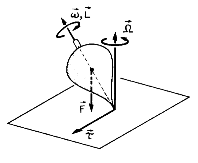
Figure 4.2: A rapidly spinning top [57].

The spinning top remains with the angular momentum conserved, $d\mathbf{L}_{0}/dt=0$, and rotation speed $\bm{\omega}$ and no torque is acted on it until it reaches the ground. When it lands, the back reaction to the weight $\mathbf{F}$ yields a torque $\bm{\tau}$ that breaks the conservation of the angular momentum. The new equation for the movement of the top is then

$$\bm{\tau}=\dfrac{d\mathbf{L}}{dt}=\bm{\Omega}\times\mathbf{L_{0}},$$ (4.11)

where $\bm{\Omega}$ is a rotation velocity different from $\bm{\omega}$, which characterizes the precession movement of the spinning top.

These computations can be generalized to a curved space-time by the principle of General Covariance, with $d/dx^{\mu}\to\nabla_{\mu}$. Nonetheless, GR predicts a different kind of precession for freely falling spinning bodies, $i.e.$ bodies where no torque or any other force is being applied. Following Ref. [7], consider a gyroscope with an intrinsic angular momentum vector $S^{\mu}=\left(S^{0},\mathbf{S}\right)$ orbiting a spherical body like the Earth. The equation of parallel transport for $S^{\mu}$ becomes

$$\nabla_{\nu}S_{\mu}=0\Leftrightarrow\dfrac{dS_{\mu}}{d\tau}=\Gamma^{\lambda}_{\mu\nu}S_{\lambda}\dfrac{dx^{\nu}}{d\tau},$$ (4.12)

where $\tau$ is the coordinate of proper time. The angular momentum vector $S_{\mu}$ is defined so as to be orthogonal to the velocity vector,

$$\dfrac{dx^{\mu}}{d\tau}S_{\mu}=0\Rightarrow S_{0}=-v^{i}S_{i},$$ (4.13)

where $i\in\{1,2,3\}$. Inserting this condition into (4.12) and multiplying it with $d\tau/dt$ yields

$$\dfrac{dS_{i}}{dt}=\Gamma^{j}_{i0}S_{j}-\Gamma^{0}_{i0}v^{j}S_{j}-\Gamma^{j}_{ik}v^{k}S_{j}-\Gamma^{0}_{ik}v^{k}v^{j}S_{j}\simeq\left({}^{(3)}\Gamma^{j}_{i0}-^{(2)}\Gamma^{0}_{i0}v^{j}+^{(2)}\Gamma^{j}_{ik}v^{k}\right)S_{j}.$$ (4.14)

The computation of this equation was done with a metric according to the PPN formalism,

$$g^{00}=-1-2\phi,\qquad\qquad g^{i0}=\zeta_{i},\qquad\qquad g^{ij}=\left(1-2\phi\right)\delta_{ij}.$$ (4.15)

The approximation from Eq. (4.14) considered only parameters of the order $\phi\sim{\cal O}(\epsilon)$ and $\zeta_{i}\sim{\cal O}(\epsilon^{3/2})$ or less, where the parameter $\epsilon$ was defined after Eq. (4.3). The number preceding some terms like ${}^{(n)}\Gamma$ represents the order of the term, $\Gamma={\cal O}(\epsilon^{n})$. Expanding the above equation with the connection terms from the metric yields

$$\dfrac{d\mathbf{S}}{dt}\simeq\dfrac{1}{2}\mathbf{S}\times\left(\nabla\times\bm{\zeta}\right)-\mathbf{S}\dfrac{\partial\phi}{\partial t}-2\left(\mathbf{v}\cdot\mathbf{S}\right)\nabla\phi-\mathbf{S}\left(\mathbf{v}\cdot\nabla\phi\right)+\mathbf{v}\left(\mathbf{S}\cdot\nabla\phi\right).$$ (4.16)

It is useful at this stage to introduce a new spin vector $\bm{\mathcal{S}}$ defined as

$$\mathbf{S}=\left(1-\phi\right)\bm{\mathcal{S}}+\dfrac{1}{2}\mathbf{v}\left(\mathbf{v}\cdot\bm{\mathcal{S}}\right)\quad\Leftrightarrow\quad\bm{\mathcal{S}}=\left(1+\phi\right)\mathbf{S}-\dfrac{1}{2}\mathbf{v}\left(\mathbf{v}\cdot\bm{S}\right),$$ (4.17)

where its equation of parallel transport to order ${\cal O}(\epsilon^{3/2})$ or less is

$$\dfrac{d\bm{\mathcal{S}}}{dt}=\dfrac{d\mathbf{S}}{dt}+\mathbf{S}\left(\dfrac{\partial\phi}{\partial t}+\mathbf{v}\cdot\nabla\phi\right)+\dfrac{1}{2}\nabla\phi\left(\mathbf{v}\cdot\mathbf{S}\right)+\dfrac{1}{2}\mathbf{v}\left(\mathbf{S}\cdot\nabla\phi\right).$$ (4.18)

$\mathbf{S}$ was considered as constant everywhere in space and $d\mathbf{v}/dt\simeq-\nabla\phi$. Inserting Eq. (4.16) into this one yields for $\bm{\mathcal{S}}$

$$\dfrac{d\bm{\mathcal{S}}}{dt}=\bm{\Omega}\times\bm{\mathcal{S}},\qquad\qquad\bm{\Omega}=\dfrac{1}{2}\nabla\times\bm{\zeta}-\dfrac{3}{2}\mathbf{v}\times\nabla\phi,$$ (4.19)

showing that $\bm{\mathcal{S}}$ precesses with angular velocity $\bm{\Omega}$.

As shown in Ref. [7], if the central spherical body is the rotating Earth at rest, then the fields $\phi$ and $\bm{\zeta}$ can be written as

$$\phi=-\dfrac{GM_{\oplus}}{r},\qquad\qquad\bm{\zeta}=\dfrac{2G}{r^{3}}\left(\mathbf{r}\times\mathbf{J}_{\oplus}\right),$$ (4.20)

where $M_{\oplus}$ and $\mathbf{J}_{\oplus}$ are the mass and angular momentum of the Earth. Inserting this fields into the precession velocity of $\bm{\mathcal{S}}$ means that it becomes

$$\bm{\Omega}=3G\dfrac{\mathbf{r}\left(\mathbf{r}\cdot\mathbf{J}_{\oplus}\right)}{r^{5}}-G\dfrac{\mathbf{J}_{\oplus}}{r^{3}}+3GM_{\oplus}\dfrac{\mathbf{r}\times\mathbf{v}}{2r^{3}},$$ (4.21)

where the last term depends only on the mass of the earth and not on its spin and it is called geodetic precession.

The geodetic precession effect is a direct consequence of the GR theory in the orbit of the Earth and it was observationally checked by the Gravity Probe B (GPB) experiment. This experiment consisted in a satellite orbiting the Earth containing a telescope focused to the binary star HR8703, from the Pegasus constellation, to use as a position reference, and four extremely precise gyroscopes (four in order to decrease the data error). The spin axis of the gyroscopes is set to be aligned with the guide star during a certain period of time. At the end of it, the change in the precession of the spin axis alignment reveals the predicted geodetic effect. The display of the experiment is shown in figure 4.3, which also shows another effect predicted by GR that was tested in the same experiment $-$ the frame-dragging effect.

The GPB confirmed the geodetic effect as a correct prediction of GR with $0,28\%$ of accuracy [58]. Interactions between random patches of electrostatic potential in the gyroscopes did not allow for such a high precision in the frame-dragging effect [59].

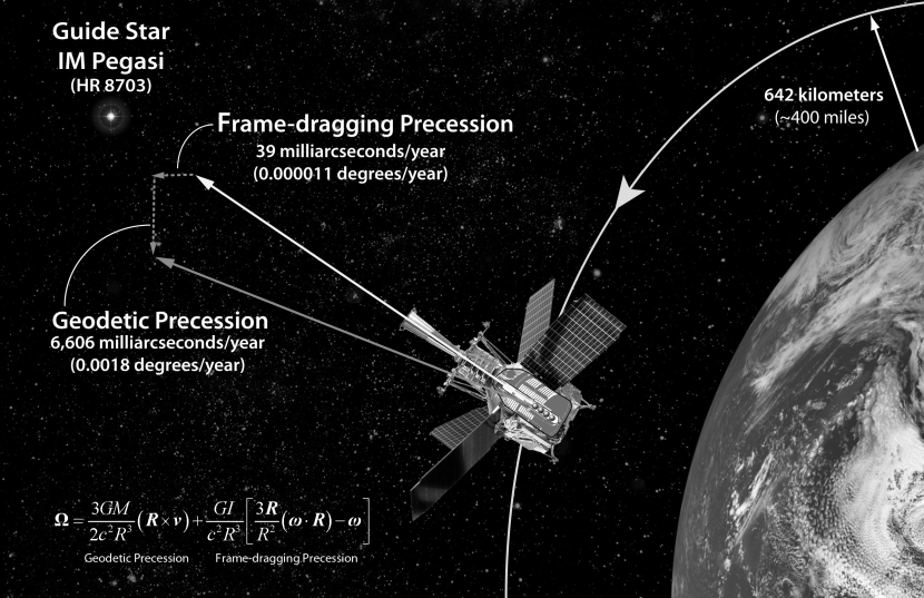
Figure 4.3: Representation of the GPB experiment and the geodetic effect prediction [60].

Although not as accurate as the GPB experiment, tests on LLR also confirm the geodetic precession, with a 1% accuracy [4]. LLR involves the analysis of data coming from lasers emitted from the Earth to the Moon and then reflected back to the Earth. This LLR experiment also yields a specific constraint on Yukawa modifications to the ISL, equivalent to the perigee precession of LAGEOS II [3], which will be mentioned in a later section.

Chapter 5 Short Range Solar System impact of a NMC

The contents of the following chapters include original work and are completely based in Ref. [1].

In this chapter the procedure from section 2.3.2 to assess the short range Solar System impact of $f(R)$ theories will be followed, where a NMC model will be considered instead. This is done considering that the additional degree of freedom arising from a non-trivial $f(R)$ function is sufficiently massive so that its effects are not extremely long-ranged, and as such the background cosmological setting can be neglected $-$ this point (which shall be developed in the following sections) shows that the method is complementary to the recent study on the compatibility between cosmological and Solar System dynamics exposed in section 3.3.

The action functional used is again the one from Eq. (3.1), with the field equations (3.2). It is once more assumed that matter behaves as dust, with the energy momentum tensor described by Eq. (2.60), and that the mass density respects the conditions from Eq. (2.61).

As before, the metric used is one that describes the spacetime around a spherical star like the Sun and it is given by the following perturbation of the Minkowski metric, in spherical coordinates:

$$ds^{2}=-\left[1+2\Psi\left(r\right)\right]c^{2}dt^{2}+\left[1+2\Phi(r)\right]dr^{2}+r^{2}d\Omega^{2},$$ (5.1)

where $\Psi$ and $\Phi$ are perturbing functions such that $\left|\Psi(r)\right|\ll 1$ and $\left|\Phi(r)\right|\ll 1$. For the purpose of the present work the functions $\Psi$ and $\Phi$ will be computed at order ${\cal O}(1/c^{2})$. The functions $f^{i}(R)$ are assumed to admit the following Taylor expansions around $R=0$, which coincide with the forms used in the NMC preheating study from section 3.2:

$$f^{1}(R)=2\kappa\left(R+\dfrac{R^{2}}{6m^{2}}\right)+{\cal O}(R^{3}),\qquad\qquad f^{2}(R)=2\xi\dfrac{R}{m^{2}}+{\cal O}(R^{2}),$$ (5.2)

where $m$ is a characteristic mass scale and $\xi$ a dimensionless parameter specific of the NMC, indicating the relative strength of the latter with respect to the quadratic term in $f^{1}(R)$.

It should be noted that the Cosmological Constant is dropped, consistent with the assumption that the metric is asymptotically flat — i.e. no cosmological background with a time-dependent, non-vanishing curvature $R_{0}\neq 0$ is assumed, contrary to what was considered in section 3.3.

5.1 Solution of linearized modified field equations

5.1.1 Solution for the curvature $R$

The trace of the field equations (3.2) is

$$\left(f^{1}_{R}+2f^{2}_{R}{\cal L}_{m}\right)R-2f^{1}=-3\square\left(f^{1}_{R}+2f^{2}_{R}{\cal L}_{m}\right)+\left(1+f^{2}\right)T.$$ (5.3)

After expanding the trace with the respective expressions, the equation is linearized: this is done by neglecting terms of order ${\cal O}(1/c^{3})$ or smaller, which then yields the following equation,

$$\nabla^{2}R-m^{2}R=-\dfrac{8\pi G}{c^{2}}m^{2}\left[\rho-6\left(\dfrac{2\xi}{m^{2}}\right)\nabla^{2}\rho\right].$$ (5.4)

The variable substitution $u=rR$, enables the more straightforward expression

$$\dfrac{d^{2}u(r)}{dr^{2}}-m^{2}u(r)=s(r),$$ (5.5)

where

$$s(r)=-\dfrac{8\pi G}{c^{2}}m^{2}r\left[\rho-6\left(\dfrac{2\xi}{m^{2}}\right)\nabla^{2}\rho\right],$$ (5.6)

is the source function.

The boundary conditions on $u(r)$ are the ones listed after Eq. (2.64). The Green function of Eq. (5.5) solves the following equation in the sense of distributions

$$\dfrac{d^{2}G(r,r^{\prime})}{dr^{2}}-m^{2}G(r,r^{\prime})=\delta(r-r^{\prime}),$$ (5.7)

where $\delta(r-r^{\prime})$ is the Dirac delta distribution. The Green function $G(r,r^{\prime})$ is used to determine the solution of the curvature equation in the form (5.5) by means of the integral $u(r)=\int^{R_{S}}_{0}G(r,r^{\prime})s(r^{\prime})dr^{\prime}$. Due to the different boundary conditions, the curvature is written as a twofold solution:

$$R(r)=\left\{\begin{array}[]{l l}R^{\uparrow}(r)&\quad\text{if }r>R_{S}\\ \\ R^{\downarrow}(r)&\quad\text{if }0\leq r\leq R_{S}\end{array}\right.,$$ (5.8)

where $R^{\downarrow}(r)$ is the curvature inside the star,

$$R^{\downarrow}(r)=-\dfrac{4\pi G}{c^{2}m}\left[\dfrac{e^{-mr}}{r}I_{1}(r)+\dfrac{2\sinh(mr)}{r}I_{2}(r)\right],$$ (5.9)

the quantities $I_{1}(r)$ and $I_{2}(r)$ have been computed by using the properties (2.61) of the mass density $\rho(r)$ and are given by

$$I_{1}(r) = 2\left(12\xi-1\right)m^{2}\int^{r}_{0}\sinh(mr^{\prime})r^{\prime}\rho(r^{\prime})dr^{\prime}-24\xi\cosh(mr)mr\rho(r),$$ (5.10)

$$I_{2}(r) = (12\xi-1)m^{2}\int^{R_{S}}_{r}e^{-mr^{\prime}}r^{\prime}\rho(r^{\prime})dr^{\prime}-12\xi e^{-mr}mr\rho(r),$$

and $R^{\uparrow}(r)$ is the curvature outside the star, given by

$$R^{\uparrow}(r)=\dfrac{2GM_{S}}{c^{2}r}m^{2}\left(1-12\xi\right)A(m,R_{S})e^{-mr},$$ (5.11)

with $M_{S}$ the mass of the spherical body and $A(m,R_{S})$ a form factor defined as

$$A(m,R_{S})=\dfrac{4\pi}{mM_{S}}\int^{R_{S}}_{0}\sinh(mr)r\rho(r)dr,$$ (5.12)

which will be discussed in a subsequent section.

The expression (5.11) vanishes as $r\rightarrow\infty$ and it is considered to be valid only at Solar System scales, since spacetime should assume a De Sitter metric with curvature $R_{0}\neq 0$ at cosmological scales. Note also that in the limit $m\rightarrow 0$ then $R^{\uparrow}(r)\rightarrow 0$ for any $r>R_{S}$.

5.1.2 Solution for $\Psi$

The $tt$ component of the Ricci tensor at order ${\cal O}(1/c^{2})$ is given by

$$R_{tt}=\dfrac{2\Psi^{\prime}}{r}+\Psi^{\prime\prime}+{\cal O}\left(\dfrac{1}{c^{3}}\right)=\nabla^{2}\Psi+{\cal O}\left(\dfrac{1}{c^{3}}\right).$$ (5.13)

Then, neglecting all terms smaller than ${\cal O}(1/c^{2})$ in the $tt$ component of the field equations (3.2), and using the curvature equation (5.4), the equation ruling $\Psi$ becomes:

$$\nabla^{2}\Psi=\dfrac{c^{2}}{3k}\rho-\dfrac{R}{6}.$$ (5.14)

This is solved outside the spherical body, $r\geq R_{S}$, by decomposing it into a sum,

$$\nabla^{2}\Psi=\nabla^{2}\Psi_{0}+\nabla^{2}\Psi_{1},$$ (5.15)

where

$$\nabla^{2}\Psi_{0}=\dfrac{c^{2}}{3k}\rho\leavevmode\nobreak\ \leavevmode\nobreak\ \leavevmode\nobreak\ \leavevmode\nobreak\ ,\leavevmode\nobreak\ \leavevmode\nobreak\ \leavevmode\nobreak\ \leavevmode\nobreak\ \nabla^{2}\Psi_{1}=-\dfrac{R}{6}.$$ (5.16)

The first equation is easily solved using the divergence theorem, which gives

$$\Psi_{0}(r)=-\dfrac{4}{3}\dfrac{GM_{S}}{c^{2}r}.$$ (5.17)

The second one is more cumbersome: a tedious integration eventually shows that

$$\Psi_{1}(r)=\dfrac{GM_{S}}{3c^{2}r}\left[1-\left(1-12\xi\right)A(m,R_{S})e^{-mr}\right],$$ (5.18)

so that for $r\geq R_{S}$ the solution is

$$\Psi(r)=-\dfrac{GM_{S}}{c^{2}r}\left[1+\left(\dfrac{1}{3}-4\xi\right)A(m,R_{S})e^{-mr}\right].$$ (5.19)

5.1.3 Solution for $\Phi$

By the same token, being the mass distribution static, the expressions

$$R_{rr}=\dfrac{2}{r}\Phi^{\prime}-\Psi^{\prime\prime}+{\cal O}\left(\dfrac{1}{c^{3}}\right)\leavevmode\nobreak\ \leavevmode\nobreak\ \leavevmode\nobreak\ \leavevmode\nobreak\ ,\leavevmode\nobreak\ \leavevmode\nobreak\ \leavevmode\nobreak\ \leavevmode\nobreak\ T_{rr}=0,$$ (5.20)

can be inserted into the $rr$ component of the field equations, along with the $f^{i}(R)$ expressions from (5.2), obtaining

$$2\Phi^{\prime}-r\Psi^{\prime\prime}-\dfrac{rR}{2}+\dfrac{2R^{\prime}}{3m^{2}}-\dfrac{4\xi c^{2}}{m^{2}k}\rho^{\prime}=0.$$ (5.21)

This equation is easily integrated outside the spherical body, $r\geq R_{S}$, leading to

$$\Phi(r)=\dfrac{GM_{S}}{c^{2}r}\left[1-\left(\dfrac{1}{3}-4\xi\right)A(m,R_{S})e^{-mr}(1+mr)\right].$$ (5.22)

In the GR limit, $\xi=0$ and $m\to\infty$, the exponential term in both $\Psi$ and $\Phi$ vanishes and the weak-field approximation of the Schwarzschild metric is recovered, as expected.

5.2 Discussion of Yukawa potential

As it has been shown, from the $tt$ component of the metric it is possible to identify a Newtonian potential plus a Yukawa perturbation:

$$U(r)=-\dfrac{GM_{S}}{r}\left(1+\alpha A(m,R_{S})e^{-r/\lambda}\right),$$ (5.23)

defining the characteristic length $\lambda=1/m$ and the strength of the Yukawa addition

$$\alpha=\dfrac{1}{3}-4\xi,$$ (5.24)

so that, if $\xi=0$, the Yukawa strength for pure $f(R)$ theories from chapter 2 is obtained, $\alpha=1/3$; it should also be noticed that a positive NMC (as assumed in Refs. [36, 61]) yields $\alpha\leq 1/3$. Strikingly, a NMC with $\xi=1/12$ cancels the Yukawa contribution.

5.2.1 The form factor $A(m,R_{S})$

As defined before, the form factor is

$$A(m,R_{S})=\dfrac{4\pi}{mM_{S}}\int_{0}^{R_{S}}\sinh(mr)r\rho(r)dr.$$ (5.25)

This dimensionless form factor was found by integrating the field equations of NMC gravity but it is not specific of the NMC gravity nor of $f(R)$ theories of this kind, as it was shown in section 4.1. This form factor can then be evaluated in several ways, according to the function of mass density $\rho(r)$. Taking the limit of a point source, $r\to 0$ allows to expand around $mr\ll 1$, so that $\sinh\left(mr\right)\approx mr[1+(mr)^{2}/6]$ and

$$A(m,R_{S})\approx\dfrac{4\pi}{M_{S}}\int^{R_{S}}_{0}\left[1+\dfrac{(mr)^{2}}{6}\right]r^{2}\rho(r)dr=1+\dfrac{2m^{2}\pi}{3M_{S}}\int^{R_{S}}_{0}r^{4}\rho(r)dr\sim 1.$$ (5.26)

This can be verified explicitly by making all computations with a test mass density (such as a uniform profile) and, in the end, taking the limit $R_{S}\to 0$. Indeed, taking

$$\rho_{0}=\dfrac{3M_{S}}{4\pi R_{S}^{3}}$$ (5.27)

then

$$A(m,R_{S})=3\dfrac{mR_{S}\cosh(mR_{S})-\sinh(mR_{S})}{(mR_{S})^{3}},$$ (5.28)

which admits the limiting cases

$$A(m,R_{S}) \approx 1+\dfrac{(mR_{S})^{2}}{10}\sim 1\leavevmode\nobreak\ \leavevmode\nobreak\ ,\leavevmode\nobreak\ \leavevmode\nobreak\ mR_{S}\ll 1,$$ (5.29)

$$A(m,R_{S}) \approx \dfrac{3}{2}\dfrac{e^{mR_{S}}}{(mR_{S})^{2}}\leavevmode\nobreak\ \leavevmode\nobreak\ ,\leavevmode\nobreak\ \leavevmode\nobreak\ mR_{S}\gg 1.$$

If the central body is the Sun (with radius $R_{\odot}$), the more accurate density NASA profile [62] can instead be considered (which obeys condition $\rho(R_{\odot})=0$, while $(d\rho/dr)(R_{\odot})\simeq 0$),

$$\rho(r)=\rho_{0}\bigg{[}1-5.74\left(\dfrac{r}{R_{\odot}}\right)+11.9\left(\dfrac{r}{R_{\odot}}\right)^{2}-10.5\left(\dfrac{r}{R_{\odot}}\right)^{3}+3.34\left(\dfrac{r}{R_{\odot}}\right)^{4}\bigg{]},$$ (5.30)

obtaining

$$A(m,R_{\odot}) = x^{-7}[4.6\times 10^{4}x+2.1\times 10^{3}x^{3}+(2.7\times 10^{4}+131x^{2})x\cosh x-$$

$$(7.3\times 10^{4}+3.6\times 10^{3}x^{2}-14.6x^{4})\sinh x],$$

(with $x=mR_{\odot}$, for brevity), with the limiting cases

$$A(m,R_{\odot}) \approx 1+6\times 10^{-2}(mR_{\odot})^{2}\sim 1\leavevmode\nobreak\ \leavevmode\nobreak\ ,\leavevmode\nobreak\ \leavevmode\nobreak\ mR_{\odot}\ll 1,$$

$$A(m,R_{\odot}) \approx \ 7.3\dfrac{e^{mR_{\odot}}}{(mR_{\odot})^{3}}\leavevmode\nobreak\ \leavevmode\nobreak\ ,\leavevmode\nobreak\ \leavevmode\nobreak\ mR_{\odot}\gg 1.$$ (5.32)

Both forms for $A(m,R_{\odot})$ are plotted in Fig. 5.1, showing that it grows with $mR_{\odot}$. Although this effectively boosts the form factor for values of lengthscale $\lambda\ll R_{\odot}$, the contribution from the Yukawa term in Eq. (5.23) is nevertheless suppressed by the factor $\exp(-r/\lambda)$.

5.2.2 PPN Parameters

Similarly to the present considerations, the PPN formalism posits an expansion of the metric elements and other quantities (energy-momentum tensor, equations of motion, etc.) in powers of $1/c^{2}$, as it was introduced in section 4.2.

Clearly, such a formalism is incompatible with the presence of a Yukawa term in the gravitational potential, since the latter cannot be expanded in powers of $1/r$; furthermore, the discussion after Eq. (5.11) highlights that, in the limit $m\to 0$, the background cosmological curvature must be considered and the asymptotically flat Ansatz (5.1) for the metric cannot be assumed: this was performed in section 3.3, as already mentioned.

Nevertheless, for consistency, what happens if the condition $mr\ll 1$ is valid throughout the region of interest (e.g. the Solar System) can be considered: in this case, the metric (5.1) with the solutions (5.19) and (5.22) is well approximated by

$$ds^{2}=-\left[1-\dfrac{2GM_{S}}{c^{2}r}\left(\dfrac{4}{3}-4\xi\right)\right]c^{2}dt^{2}+\left[1+\dfrac{2GM_{S}}{c^{2}r}\left(\dfrac{2}{3}+4\xi\right)\right]dr^{2}+r^{2}d\Omega^{2},$$ (5.33)

which yields

$$\gamma=\dfrac{1}{2}\dfrac{1+6\xi}{1-3\xi}.$$ (5.34)

In the absence of a NMC, $\xi=0$, this yields $\gamma=1/2$, a strong departure from GR that is disallowed by current experimental bounds, $\gamma=1+(2.1\pm 2.3)\times 10^{-5}$ [48]. This apparent disagreement between $f(R)$ theories and observations was already noted (as discussed in section 2.3), and can be avoided if the additional degree of freedom arising from a non-linear $f(R)$ function is massive enough.

The expression above appears to show that a NMC allows $f(R)$ theories to remain compatible with observations, as long as $\xi=1/12$ — which is just a restatement of the previously obtained result. Again, the path towards obtaining the $\gamma$ PPN parameter depicted above is presented for illustration only, as it relies on an approximation of a Yukawa perturbation and disregards the fact that, in the limit $mr\ll 1$, the background cosmological dynamics cannot be neglected. As such, no conclusions can be drawn from comparison with the experimental bound on $\gamma$ mentioned above.

5.3 Experimental constraints to NMC gravity parameters

The Yukawa potential (5.23) is not new in physics as an alternative way to account for deviations from Newtonian gravity or other forces of nature, as it was shown in section 4.1. Fig. 5.2 shows the exclusion plot for the phase space $(\lambda,\alpha)$, which may be used to constrain the phase space of the model (3.1) under scrutiny.

In doing so, it is important to recall that the results obtained in Eqs. (5.19,5.22,5.23) are not exact, but only accurate to order ${\cal O}(c^{-2})$, and are based upon the assumption of a perturbation to a Minkowski metric: a future analysis should expand this framework to also include terms ${\cal O}(c^{-4})$, as well as establish some matching criteria between the static, spherically symmetric spacetime here considered and the evolving background spacetime [63] (see also Ref. [64]). Indeed, Ref. [65] has found that in $f(R)$ theories, ${\cal O}(c^{-4})$ terms can arise that are not exponentially suppressed, and as such may play a role at large distances, particularly if the ${\cal O}(c^{-2})$ Yukawa interaction here obtained is short-ranged.

From Fig. 5.2 (as discussed after (5.24)), it is seen that a NMC with $\xi=1/12$ cancels this contribution, as shown by the values of $|\alpha|\to 0$ overlaid on the exclusion plot. Also, it should be noticed that large values of $\xi$ lead to a large, negative strength $\alpha\sim-4\xi$ (the cases $\xi=25$ and $\xi=2500$ are shown).

This plot may be transformed into the phase space $(m,\xi)$ of the model under scrutiny, (5.2), using

$$m=\frac{1}{\lambda},\qquad\qquad\xi=\frac{1}{12}-\frac{\alpha}{4},$$ (5.35)

to get the exclusion plot depicted in Fig. 5.3.

Further insight is obtained by casting the NMC presented in Eq. (5.2) as

$$f^{2}(R)=\frac{R}{6M^{2}},$$ (5.36)

so that it is characterized by a distinct mass scale $M$, instead of the relative strength parameter $\xi$: by making the transformation $\xi=(m/M)^{2}/12$, the suggestive form

$$\alpha=\dfrac{1}{3}\left[1-\left(\dfrac{m}{M}\right)^{2}\right],$$ (5.37)

is thus obtained, which, inverting, allows to plot the exclusion plot for the phase space $(m,M)$ in Fig. 5.4.

Figure 5.1: Numerical plot of form factor $A(m,R_{\odot})$ for a constant density (full) and fourth-order density profile for the Sun, Eq. (5.30) (dashed).

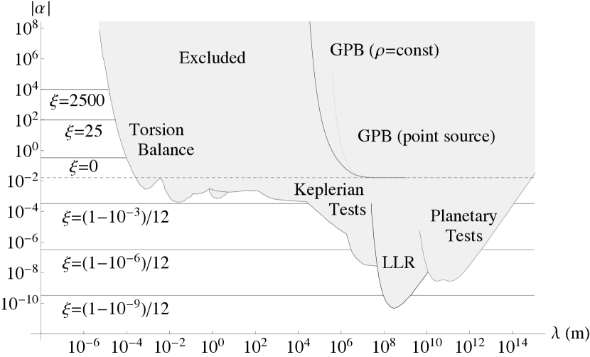
Figure 5.2: Yukawa exclusion plot for $\alpha$ and $\lambda$. Adapted from Refs. [51, 52].

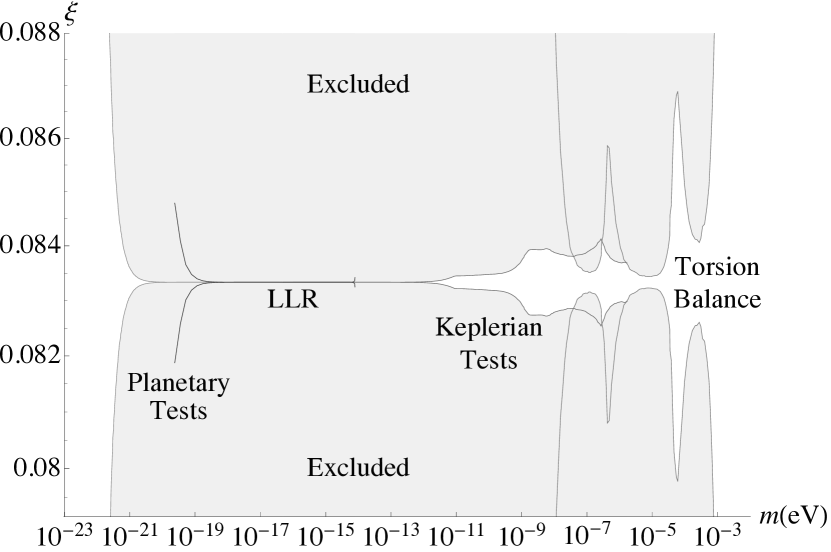
Figure 5.3: Exclusion plot for the dimensionless relative strength $\xi$ and characteristic mass scale $m$.

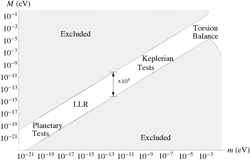
Figure 5.4: Exclusion plot for the characteristic mass scales $M$ and $m$.

Figs. 5.2-5.4 show us that, if $m$ falls within the range $10^{-22}\leavevmode\nobreak\ {\rm eV}<m<1\leavevmode\nobreak\ {\rm meV}$ (corresponding to lengthscales $\lambda$ ranging from the millimeter to Solar System scales), then the strong constraints available on the Yukawa strength, $|\alpha|\ll 1$, require that $\xi\sim 1/12$ — or, equivalently, that both characteristic mass scales are very similar, $m\sim M$.

5.3.1 Geodetic precession

In this section it is assumed that the Earth can be approximated as a spherically symmetric body. In order to assess the impact of the obtained expression for $\Phi(r)$, Eq. (5.22), we now consider a gyroscope in a circular orbit with radius $r$ around the Earth. According to section 4.3, the intrinsic angular momentum vector $S^{\mu}=\left(S^{0},\mathbf{S}\right)$ precesses according to the equation of parallel transport:

$$\frac{dS^{\mu}}{d\tau}=-\Gamma^{\mu}_{\nu\sigma}S^{\nu}\frac{dx^{\sigma}}{d\tau},$$ (5.38)

where $\tau$ is the proper time. For convenience, the metric tensor around the Earth is written in rectangular isotropic coordinates,

$$ds^{2}=-\left[1-\frac{2GM_{S}}{c^{2}r}\left(1+\alpha A(m,R_{S})e^{-mr}\right)\right]c^{2}dt^{2}+\left[1+\frac{2GM_{S}}{c^{2}r}\left(1-\alpha A(m,R_{S})e^{-mr}\right)\right]dV^{2}.$$ (5.39)

The standard method of computation of gyroscope precession in GR yields for the secular part of $d\mathbf{S}/dt$ in NMC gravity, in the slow motion and weak field approximation,

$$\left(\dfrac{d\mathbf{S}}{dt}\right)_{{\rm sec}}=\frac{3}{2}\frac{GM_{S}}{c^{2}r^{3}}\left[1-\frac{\alpha A(m,R_{S})}{3}(1+mr)e^{-mr}\right]\left(\mathbf{r}\times\mathbf{v}\right)\times\mathbf{S},$$ (5.40)

where $\mathbf{r}$ is the radius vector of the center of mass of the gyroscope and $\mathbf{v}$ is its velocity vector. Imposing the equality between the acceleration $v^{2}/r$ of the center of mass of the gyroscope and the sum of the Newton plus Yukawa forces per unit mass yields

$$vr=\sqrt{GM_{S}r[1+\alpha A(m,R_{S})(1+mr)e^{-mr}]}.$$ (5.41)

Since $\left(d\mathbf{S}/dt\right)_{{\rm sec}}=\bm{\Omega}_{G}\times\mathbf{S}$, the angular velocity vector $\bm{\Omega}_{G}$ of geodetic precession is given by

$$\bm{\Omega}_{G}=\frac{3}{2}\frac{\left(GM_{S}\right)^{3/2}}{c^{2}r^{5/2}}\left[1+\alpha A(m,R_{S})(1+mr)e^{-mr}\right]^{1/2}\times\left[1-\frac{\alpha A(m,R_{S})}{3}(1+mr)e^{-mr}\right]\mathbf{n},$$ (5.42)

where $\mathbf{n}$ is the unit vector perpendicular to the plane of the orbit. If $\xi=0$, the above expression reduces to the case for $f(R)$ models, as expected [33].

5.3.1.A Gravity Probe B results

As it was already mentioned, the final results of the GPB experiment report an accuracy of 0.28% in the measurement of geodetic precession [58]. This corresponds to the following constraint on NMC gravity parameters:

$$\left|\frac{\Omega_{G}-\Omega_{G}^{{\rm GR}}}{\Omega_{G}^{{\rm GR}}}\right|<0.0028,$$ (5.43)

where only the modulus of angular velocity is considered, and $\Omega_{G}^{{\rm GR}}$ denotes the value of geodetic precession in GR. Substituting the expression of NMC geodetic precession in this constraint we find

$$\Big{|}\sqrt{1+\alpha A(m,R_{S})(1+mr)e^{-mr}}\left[1-\frac{\alpha A(m,R_{S})}{3}(1+mr)e^{-mr}\right]-1\Big{|}<0.0028.$$ (5.44)

Defining $x\equiv\alpha A(m,R_{S})(1+mr)e^{-mr}$, this is written as

$$\Big{|}\sqrt{1+x}\left(1-\frac{x}{3}\right)-1\Big{|}<0.0028.$$ (5.45)

If $x\gg 1$, then $|x|<0.04$, which is contradictory. Since substitution shows that $x\sim 1$ breaks the above relation, the only natural constraint left is $x\ll 1$, so that a first order expansion of the above yields $|x|<0.0168$. This last condition is translated as

$$|\alpha|<\dfrac{0.0168}{1+mr}\dfrac{e^{mr}}{A(m,R_{S})}.$$ (5.46)

In order to satisfy the assumption (2.61) of continuity of mass density and its derivative across the surface of the Earth, it is possible to model the density with a constant value in an interior region (i.e. mantle plus core) and a sharp transition in a thin crustal layer. When the thickness of the latter tends to zero, the form factor $A(m,R_{S})$ converges to the value corresponding to the uniform density model, Eq. (5.29), hence the inequality (5.46) reads

$$|\alpha| < 0.0168\leavevmode\nobreak\ \leavevmode\nobreak\ ,\leavevmode\nobreak\ \leavevmode\nobreak\ mR_{\oplus}\ll 1\leavevmode\nobreak\ \leavevmode\nobreak\ ,$$ (5.47)

$$|\alpha| < 0.0112\dfrac{mR_{\oplus}^{2}}{r}e^{m(r-R_{\oplus})}\leavevmode\nobreak\ \leavevmode\nobreak\ ,\leavevmode\nobreak\ \leavevmode\nobreak\ mR_{\oplus}\gg 1\leavevmode\nobreak\ \leavevmode\nobreak\ ,$$

where $R_{\oplus}\approx 6371$ km is the radius of the Earth. Knowing that the GPB satellite orbits the Earth at a height of $\sim 650$ km, this condition can be plotted in the $(\lambda,\alpha)$ exclusion plot, as shown in Fig. 5.2. It is found that the condition is well-within the already excluded phase space, so that the current bounds on geodetic precession do not add any new constraint on the model parameters.

5.3.1.B Measurement of the LAGEOS II perigee precession

A recent analysis of the perigee precession of the LAGEOS II satellite reported a much stronger constraint on the strength of the Yukawa perturbation, $|\alpha|\simeq|(1.0\pm 8.9)|\times 10^{-12}$, at a range $\lambda=1/m=6081$ km, very close to one Earth radius [3]: a striking improvement over previous Earth-LAGEOS and Lunar-LAGEOS measurements (at the level of $10^{-5}$ and $10^{-8}$), and comparable to the Lunar Laser Ranging constraint on $\alpha$ for $\lambda\sim 60R_{\oplus}$ [4].

Non-gravitational perturbations, mainly thermal perturbative effects, can strongly affect the precession of the perigee of LAGEOS II: in [3], solar radiation pressure and Earth’s albedo are taken into account, while Rubincam and Yarkovsky-Schach (YS) thermal effects (which need the satellite spin modeling) have not been considered. Nevertheless, the residuals in the perigee rate of the satellite are fitted with a linear trend (which represents the secular total GR precession) plus four periodic terms which correspond to the main spectral lines of the unmodeled YS effect [3].

This said, if the impressive bound on $\alpha$ quoted above is indeed confirmed, no qualitative changes occur in the previous analysis: as long as the Yukawa coupling strength lies below unity sufficiently, then the NMC parameter must be $\xi\sim 1/12\rightarrow M\sim m$, so that lowering the upper bound on the former only brings the two mass scales of the functions $f^{1}(R)$ and $f^{2}(R)$ closer together.

Chapter 6 Discussion and Outlook

In this work it has been computed the effect of a NMC model, specified by (5.2), in a perturbed weak-field Schwarzschild metric, as depicted in Eq. (5.19) and (5.22). In the weak-field limit, this translates into a Yukawa perturbation to the usual Newtonian potential, with characteristic range and coupling strength

$$\lambda=\dfrac{1}{m}\leavevmode\nobreak\ \leavevmode\nobreak\ \leavevmode\nobreak\ \leavevmode\nobreak\ ,\leavevmode\nobreak\ \leavevmode\nobreak\ \leavevmode\nobreak\ \leavevmode\nobreak\ \alpha=\left(\dfrac{1}{3}-4\xi\right)=\dfrac{1}{3}\left[1-\left(\dfrac{m}{M}\right)^{2}\right]\leavevmode\nobreak\ \leavevmode\nobreak\ .$$ (6.1)

This result is quite natural and can be interpreted straightforwardly: a minimally coupled $f(R)$ theory introduces a new massive degree of freedom (as hinted by the equivalence with a scalar-tensor theory [66, 67, 68]), leading to a Yukawa contribution with characteristic lengthscale $\lambda=1/m$ and coupling strength $\alpha=1/3$.

The introduction of a NMC has no dynamical effect in the vacuum, as there is no matter to couple the scalar curvature to: as a result, it is not expected any modification in the range of this Yukawa addition. Conversely, a NMC has an impact on the description of the interior of the central body leading to a correction to the latter’s coupling strength (which has a negative sign since ${\cal L}_{m}=-\rho$), as mentioned in the beginning of chapter 3.

Using the available experimental constraints, it was found that, for $10^{-22}\leavevmode\nobreak\ {\rm eV}<m<1\leavevmode\nobreak\ {\rm meV}$ (i.e. the range $10^{-4}\leavevmode\nobreak\ {\rm m}<\lambda<10^{16}\leavevmode\nobreak\ {\rm m}$), where $|\alpha|\ll 1$, then the NMC parameter must be $\xi\sim 1/12$ or, equivalently, both mass scales $m$ and $M$ of the non-trivial functions $f^{1}(R)$ and $f^{2}(R)$ must be extremely close.

If this is the case, the latter relation is not interpreted as an undesirable fine-tuning, but instead is suggestive of a common origin for both non-trivial functions $f^{1}(R)$ and $f^{2}(R)$, in line with the argument stating that the model (3.1) should arise as a low energy phenomenological approximation to a yet unknown fundamental theory of gravity.

Furthermore, one notices that the result $\xi=1/12$ is directly equivalent to the action

$$S=\int\left(1+\dfrac{R}{6m^{2}}\right)\left(\kappa R+{\cal L}_{m}\right)\sqrt{-g}d^{4}x,$$ (6.2)

and the main result of this work can be recast in a more appealing way: if an analytical (around $R=0$) NMC model leads to a massive degree of freedom with a short range which falls within the currently observable region $1\leavevmode\nobreak\ {\rm mm}\lesssim\lambda\lesssim 10^{15}\leavevmode\nobreak\ {\rm m}$, then it must correspond to a global factorisation of the Einstein-Hilbert Lagrangian, as shown above. Further studies based on this insight, and its extension to higher order couplings, can be realised by considering the so-called $F(R,{\cal L}_{m})$ set of theories [69].

Conversely, for values of $m$ (or $\lambda$) away from the range mentioned above the Yukawa coupling strength, $\alpha$ can be much larger than unity, so that $\xi$ can assume any value and the mass scales $m$ and $M$ can differ considerably.

In particular, the Starobinsky inflationary model, which requires the much heavier mass scale $m\approx 3\times 10^{13}$ GeV $\sim 10^{-6}M_{P}$, manifests itself at a lengthscale $\lambda\sim 10^{-29}\leavevmode\nobreak\ {\rm m}$. This implies that the generalized preheating scenario posited in section 2.2.1 and in Ref. [40], which requires $1<\xi<10^{4}$, is thus completely allowed by experiment and unconstrained by this work.

By computing the perturbation induced on geodetic precession, it was found that no significant new constraint arises, as this is already included in the existing Yukawa exclusion plot. Furthermore, even considering the much improved precision claimed in a recent study of LAGEOS II — or, for that matter, any further refinement of $|\alpha|\ll 1$ $-$, no qualitatively new results arise, since this only bridges the gap between $m$ and $M$ (i.e. narrows the value of $|\xi-1/12|$).

Finally, a word is due for the so-called chameleon mechanism, first posited in Ref. [70, 71, 72, 73], as discussed in Ref. [33] in relation to $f(R)$ theories. This non-linear effect goes beyond the linear expansion of the modified field equations, and relies on the equivalence between $f(R)$ theories and a scalar-tensor theory with a scalar field $\phi$ proportional to $f_{R}$, which appears non-minimally coupled to the matter Lagrangian density (in the Einstein frame) [66, 67, 68, 9].

As it turns out, the effective potential of this scalar field can be written as $V_{eff}(\phi)=V(\phi)+e^{a\phi}\rho$ (with $a$ an appropriate constant), so that the position of its minimum depends on the density $\rho$, and the mass for the scalar field grows with the density: this is particularly relevant in a cosmological context, where the low background density yields a light, long-ranged field.

Given the above, Ref. [33] speculates that further computations allowing for this non-linear effect could lead to different constraints on the mass scale $m$ of the adopted quadratic form for $f^{1}(R)$: quite naturally, the inclusion of a direct coupling between curvature (vis-à-vis the scalar field) and matter only heightens this possibility.

Clearly, this prompts for a future study of the relation between this chameleon mechanism and a NMC model, in the framework of its equivalence with a multi-scalar-tensor theory as shown in section 3.1. Nonetheless, one should notice that for $\xi=1/12$ the chameleon mechanism is not necessary.

References

- Castel-Branco et al. [2014] N. Castel-Branco, J. Páramos, and R. March, “Perturbation of the metric around a spherical body from a nonminimal coupling between matter and curvature,” (2014), arXiv:1403.7251 [astro-ph.CO] .
- Will [2006] C. M. Will, “The Confrontation between general relativity and experiment,” Living Rev.Rel. 9, 3 (2006), arXiv:gr-qc/0510072 [gr-qc] .
- Lucchesi and Peron [2010] D. M. Lucchesi and R. Peron, “Accurate Measurement in the Field of the Earth of the General-Relativistic Precession of the LAGEOS II Pericenter and New Constraints on Non-Newtonian Gravity,” Phys. Rev. Lett. 105, 231103 (2010).
- Muller et al. [2005] J. Muller, J. G. Williams, and S. G. Turyshev, “Lunar laser ranging contributions to relativity and geodesy,” (2005), arXiv:gr-qc/0509114 [gr-qc] .
- Walker [1935] A. G. Walker, “On Riemannian Spaces with Spherical Symmetry about a Line, and the Conditions of Isotropy in General Relativity,” The Quarterly Journal of Mathematics 6, 81 (1935).
- Robertson [1935] H. P. Robertson, “Kinematics and World-Structure,” Astrophys.J. 82, 284 (1935).
- Weinberg [1972] S. Weinberg, Gravitation and Cosmology: Principles and Applications of the General Theory of Relativity (Springer Verlag, Berlin, 1972).
- Guth [1981] A. H. Guth, “Inflationary universe: A possible solution to the horizon and flatness problems,” Phys. Rev. D 23, 347 (1981).
- Felice and Tsujikawa [2010] A. D. Felice and S. Tsujikawa, “ Theories,” Living Reviews in Relativity 13 (2010), 10.12942/lrr-2010-3.
- et al. [2009] B. et al., “CMBPol Mission Concept Study - Probing Inflation with CMB Polarization,” in AIP Conference Proceedings, Vol. 1141 (2009) pp. 10–120.
- Ade et al. [2013a] P. Ade et al. (Planck Collaboration), “Planck 2013 results. XXII. Constraints on inflation,” (2013a), arXiv:1303.5082 [astro-ph.CO] .
- Ade et al. [2014] P. Ade et al. (BICEP2 Collaboration), “BICEP2 I: Detection Of B-mode Polarization at Degree Angular Scales,” (2014), arXiv:1403.3985 [astro-ph.CO] .
- Flauger et al. [2014] R. Flauger, J. Colin Hill, and D. N. Sperger, “Toward and Understanding of Foregroud Emission in the BICEP2 Region,” (2014), arXiv:1405.7351 [astro-ph.CO] .
- J. Mortonson and Seljak [2014] M. J. Mortonson and U. Seljak, “A joint analysis of Planck and BICEP2 B modes including dust polarization uncertainty,” (2014), arXiv:1405.5857 [astro-ph.CO] .
- Kiefer [2012] C. Kiefer, Quantum Gravity (Oxford University Press, 2012).
- Bertone et al. [2005] G. Bertone, D. Hooper, and J. Silk, “Particle dark matter: Evidence, candidates and constraints,” Phys.Rept. 405, 279 (2005), arXiv:hep-ph/0404175 [hep-ph] .
- Perlmutter et al. [1999] S. Perlmutter et al. (Supernova Cosmology Project), “Measurements of Omega and Lambda from 42 high redshift supernovae,” Astrophys.J. 517, 565 (1999), arXiv:astro-ph/9812133 [astro-ph] .
- Riess et al. [1998] A. G. Riess et al. (Supernova Search Team), “Observational evidence from supernovae for an accelerating universe and a cosmological constant,” Astron.J. 116, 1009 (1998), arXiv:astro-ph/9805201 [astro-ph] .
- Ade et al. [2013b] P. Ade et al. (Planck Collaboration), “Planck 2013 results. I. Overview of products and scientific results,” (2013b), arXiv:1303.5062 [astro-ph.CO] .
- Copeland et al. [2006] E. J. Copeland, M. Sami, and S. Tsujikawa, “Dynamics of dark energy,” Int.J.Mod.Phys. D15, 1753 (2006), arXiv:hep-th/0603057 [hep-th] .
- Capozziello et al. [2005] S. Capozziello, V. F. Cardone, and A. Troisi, “Reconciling dark energy models with theories,” Phys. Rev. D 71, 043503 (2005).
- Lovelock [1971] D. Lovelock, “The Einstein tensor and its generalizations,” J.Math.Phys. 12, 498 (1971).
- Koivisto [2006] T. Koivisto, “A note on covariant conservation of energy–momentum in modified gravities,” Classical and Quantum Gravity 23, 4289 (2006).
- Brans and Dicke [1961] C. Brans and R. H. Dicke, “Mach’s Principle and a Relativistic Theory of Gravitation,” Phys. Rev. 124, 925 (1961).
- Capozziello et al. [1997] S. Capozziello, R. de Ritis, and A. A. Marino, “Some aspects of the cosmological conformal equivalence between ’Jordan frame’ and ’Einstein frame’,” Class.Quant.Grav. 14, 3243 (1997), arXiv:gr-qc/9612053 [gr-qc] .
- Faraoni et al. [1999] V. Faraoni, E. Gunzig, and P. Nardone, “Conformal transformations in classical gravitational theories and in cosmology,” Fund.Cosmic Phys. 20, 121 (1999), arXiv:gr-qc/9811047 [gr-qc] .
- Starobinsky [1980] A. Starobinsky, “A new type of isotropic cosmological models without singularity,” Physics Letters B 91, 99 (1980).
- Komatsu et al. [2009] E. Komatsu et al. (WMAP Collaboration), “Five-Year Wilkinson Microwave Anisotropy Probe (WMAP) Observations: Cosmological Interpretation,” Astrophys.J.Suppl. 180, 330 (2009), arXiv:0803.0547 [astro-ph] .
- B. et al. [1986] M. B., M. S. Morris, and W.-M. Suen, “The cosmology: Inflation without a phase transition,” Phys. Rev. D 34, 2934 (1986).
- Kofman et al. [1994] L. Kofman, A. Linde, and A. A. Starobinsky, “Reheating after inflation,” Phys. Rev. Lett. 73, 3195 (1994).
- Chiba et al. [2007] T. Chiba, T. L. Smith, and A. L. Erickcek, “Solar System constraints to general gravity,” Phys. Rev. D 75, 124014 (2007).
- Bertolami et al. [2008] O. Bertolami, F. S. N. Lobo, and J. Páramos, “Nonminimal coupling of perfect fluids to curvature,” Phys. Rev. D 78, 064036 (2008).
- Näf and Jetzer [2010] J. Näf and P. Jetzer, “On the 1/c expansion of f(r) gravity,” Phys. Rev. D 81, 104003 (2010).
- Bertolami et al. [2007] O. Bertolami, C. G. Boehmer, T. Harko, and F. S. Lobo, “Extra force in modified theories of gravity,” Phys.Rev. D75, 104016 (2007), arXiv:0704.1733 [gr-qc] .
- Harko et al. [2011] T. Harko, T. S. Koivisto, and F. S. N. Lobo, “Palatini Formulation of Modified Gravity with a Non-Minimal Curvature-Matter Coupling,” Modern Physics Letters A 26, 1467 (2011).
- Bertolami and Páramos [2008] O. Bertolami and J. Páramos, “Do theories matter?” Physical Review D 77, 084018 (2008).
- Bertolami and Páramos [2011] O. Bertolami and J. Páramos, “Mimicking the cosmological constant: Constant curvature spherical solutions in a nonminimally coupled model,” Physical Review D 84, 064022 (2011).
- Bertolami and Páramos [2013] O. Bertolami and J. Páramos, “Homogeneous spherically symmetric bodies with a nonminimal coupling between curvature and matter: the choice of the Lagrangian density for matter,” (2013), arXiv:1306.1177 [gr-qc] .
- Damour and Esposito-Farese [1992] T. Damour and G. Esposito-Farese, “Tensor multiscalar theories of gravitation,” Class.Quant.Grav. 9, 2093 (1992).
- Bertolami et al. [2011] O. Bertolami, P. Frazão, and J. Páramos, “Reheating via a generalized nonminimal coupling of curvature to matter,” Phys. Rev. D 83, 044010 (2011).
- Faraoni [2007] V. Faraoni, “Viability criterion for modified gravity with an extra force,” Physical Review D 76, 127501 (2007).
- Bertolami and Sequeira [2009] O. Bertolami and M. C. Sequeira, “Energy conditions and stability in f(R) theories of gravity with nonminimal coupling to matter,” Physical Review D 79, 104010 (2009).
- Dolgov and Kawasaki [2003] A. D. Dolgov and M. Kawasaki, “Can modified gravity explain accelerated cosmic expansion?” Physics Letters B 573, 1 (2003).
- Montelongo Garcia and Lobo [2011] N. Montelongo Garcia and F. S. N. Lobo, “Wormhole geometries supported by a nonminimal curvature-matter coupling,” Classical and Quantum Gravity 28 (2011).
- Bertolami et al. [2013] O. Bertolami, R. March, and J. Páramos, “Solar system constraints to nonminimally coupled gravity,” Phys. Rev. D 88, 064019 (2013).
- Chiba [2011] T. Chiba, “The Constancy of the Constants of Nature: Updates,” Prog.Theor.Phys. 126, 993 (2011), arXiv:1111.0092 [gr-qc] .
- Bertolami et al. [2010] O. Bertolami, P. Frazão, and J. Páramos, “Accelerated expansion from a nonminimal gravitational coupling to matter,” Phys. Rev. D 81, 104046 (2010).
- Bertotti et al. [2003] B. Bertotti, L. Iess, and P. Tortora, “A test of general relativity using radio links with the Cassini spacecraft,” Nature 425, 374 (2003).
- Capozziello et al. [2003] S. Capozziello, V. Cardone, S. Carloni, and A. Troisi, “Curvature quintessence matched with observational data,” Int.J.Mod.Phys. D12, 1969 (2003), arXiv:astro-ph/0307018 [astro-ph] .
- Fischbach and Talmadge [1999] E. Fischbach and C. L. Talmadge, The Search for Non-Newtonian Gravity (Springer Verlag, 1999).
- Adelberger et al. [2003] E. Adelberger, B. R. Heckel, and A. Nelson, “Tests of the gravitational inverse square law,” Ann.Rev.Nucl.Part.Sci. 53, 77 (2003), arXiv:hep-ph/0307284 [hep-ph] .
- Salumbides et al. [2013] E. Salumbides, W. Ubachs, and V. Korobov, “Bounds on fifth forces at the sub-Angstrom length scale,” (2013), arXiv:1308.1711 [hep-ph] .
- Adelberger et al. [2009] E. Adelberger, J. Gundlach, B. Heckel, S. Hoedl, and S. Schlamminger, “Torsion balance experiments: A low-energy frontier of particle physics,” Prog.Part.Nucl.Phys. 62, 102 (2009).
- Talmadge et al. [1988] C. Talmadge, J. P. Berthias, R. W. Hellings, and E. M. Standish, “Model-independent constraints on possible modifications of newtonian gravity,” Phys. Rev. Lett. 61, 1159 (1988).
- Nordtvedt [1968] K. Nordtvedt, “Equivalence Principle for Massive Bodies. 2. Theory,” Phys.Rev. 169, 1017 (1968).
- Will [1993] C. M. Will, Theory and experiment in gravitational physics, 2nd ed. (Cambridge University Press, Cambridge, UK; New York; USA, 1993).
- Feynman et al. [2010] R. P. Feynman, R. B. Leighton, and M. Sands, The Feynman Lectures on Physics, new millenium edition ed., Vol. 1 (Basic Books, 2010).
- Everitt et al. [2011] C. W. F. Everitt, D. B. DeBra, B. W. Parkinson, J. P. Turneaure, J. W. Conklin, M. I. Heifetz, G. M. Keiser, A. S. Silbergleit, T. Holmes, J. Kolodziejczak, M. Al-Meshari, J. C. Mester, B. Muhlfelder, V. G. Solomonik, K. Stahl, P. W. Worden, W. Bencze, S. Buchman, B. Clarke, A. Al-Jadaan, H. Al-Jibreen, J. Li, J. A. Lipa, J. M. Lockhart, B. Al-Suwaidan, M. Taber, and S. Wang, “Gravity Probe B: Final Results of a Space Experiment to Test General Relativity,” Phys. Rev. Lett. 106, 221101 (2011).
- Will [2011] C. M. Will, “Finally, results from Gravity Probe B,” Physics 4, 43 (2011).
- gpb [2014] “Gravity Probe B - MISSION STATUS,” http://einstein.stanford.edu/highlights/status1.html (2014).
- Páramos and Bastos [2012] J. Páramos and C. Bastos, “Gravitational collapse in nonminimally coupled gravity: Finite density singularities and the breaking of the no-hair theorem,” Phys. Rev. D 86, 103007 (2012).
- NAS [2014] “Space Math at NASA,” http://spacemath.gsfc.nasa.gov/ (2014).
- Clifton et al. [2013] T. Clifton, P. Dunsby, R. Goswami, and A. M. Nzioki, “On the absence of the usual weak-field limit, and the impossibility of embedding some known solutions for isolated masses in cosmologies with dark energy,” Phys. Rev. D 87, 063517 (2013).
- Sereno and Jetzer [2006] M. Sereno and P. Jetzer, “Dark matter vs. modifications of the gravitational inverse-square law. Results from planetary motion in the solar system,” Mon.Not.Roy.Astron.Soc. 371, 626 (2006), arXiv:astro-ph/0606197 [astro-ph] .
- Clifton [2008] T. Clifton, “The Parameterised Post-Newtonian Limit of Fourth-Order Theories of Gravity,” Phys.Rev. D77, 024041 (2008), arXiv:0801.0983 [gr-qc] .
- Teyssandier and Tourranc [1983] P. Teyssandier and P. Tourranc, “The Cauchy problem for the theories of gravity without torsion,” J.Math.Phys. 24 (1983).
- Schmidt [1990] H. Schmidt, “Variational derivatives of arbitrarily high order and multiinflation cosmological models,” Class.Quant.Grav. 7, 1023 (1990).
- Wands [1994] D. Wands, “Extended gravity theories and the Einstein-Hilbert action,” Class.Quant.Grav. 11, 269 (1994), arXiv:gr-qc/9307034 [gr-qc] .
- Harko and Lobo [2010] T. Harko and F. S. N. Lobo, “ gravity,” Eur. Phys. J. C 70, 373 (2010).
- Khoury and Weltman [2004a] J. Khoury and A. Weltman, “Chameleon cosmology,” Phys.Rev. D69, 044026 (2004a), arXiv:astro-ph/0309411 [astro-ph] .
- Khoury and Weltman [2004b] J. Khoury and A. Weltman, “Chameleon fields: Awaiting surprises for tests of gravity in space,” Phys. Rev. Lett. 93, 171104 (2004b).
- Waterhouse [2006] T. P. Waterhouse, “An Introduction to Chameleon Gravity,” (2006), arXiv:astro-ph/0611816 [astro-ph] .
- Brax et al. [2007] P. Brax, C. Vandebruck, and A. Davis, “A Chameleon Primer,” (2007), arXiv:0706.1024 [astro-ph] .