Online Submodular Maximization under a Matroid Constraint with Application to Learning Assignments

Abstract

Which ads should we display in sponsored search in order to maximize our revenue? How should we dynamically rank information sources to maximize the value of the ranking? These applications exhibit strong diminishing returns: Redundancy decreases the marginal utility of each ad or information source. We show that these and other problems can be formalized as repeatedly selecting an assignment of items to positions to maximize a sequence of monotone submodular functions that arrive one by one. We present an efficient algorithm for this general problem and analyze it in the no-regret model. Our algorithm possesses strong theoretical guarantees, such as a performance ratio that converges to the optimal constant of $1-1/e$. We empirically evaluate our algorithm on two real-world online optimization problems on the web: ad allocation with submodular utilities, and dynamically ranking blogs to detect information cascades. Finally, we present a second algorithm that handles the more general case in which the feasible sets are given by a matroid constraint, while still maintaining a $1-1/e$ asymptotic performance ratio.

Keywords: Submodular Functions, Matroid Constraints, No Regret Algorithms, Online Algorithms

1 Introduction

Consider the problem of repeatedly choosing advertisements to display in sponsored search to maximize our revenue. In this problem, there is a small set of positions on the page, and each time a query arrives we would like to assign, to each position, one out of a large number of possible ads. In this and related problems that we call online assignment learning problems, there is a set of positions, a set of items, and a sequence of rounds, and on each round we must assign an item to each position. After each round, we obtain some reward depending on the selected assignment, and we observe the value of the reward. When there is only one position, this problem becomes the well-studied multi-armed bandit problem (Auer et al., 2002). When the positions have a linear ordering the assignment can be construed as a ranked list of elements, and the problem becomes one of selecting lists online. Online assignment learning thus models a central challenge in web search, sponsored search, news aggregators, and recommendation systems, among other applications.

A common assumption made in previous work on these problems is that the quality of an assignment is the sum of a function on the (item, position) pairs in the assignment. For example, online advertising models with click-through-rates (Edelman et al., 2007) make an assumption of this form. More recently, there have been attempts to incorporate the value of diversity in the reward function (Radlinski et al., 2008). Intuitively, even though the best $K$ results for the query “turkey” might happen to be about the country, the best list of $K$ results is likely to contain some recipes for the bird as well. This will be the case if there are diminishing returns on the number of relevant links presented to a user; for example, if it is better to present each user with at least one relevant result than to present half of the users with no relevant results and half with two relevant results. We incorporate these considerations in a flexible way by providing an algorithm that performs well whenever the reward for an assignment is a monotone submodular function of its set of (item, position) pairs. The (simpler) offline problem of maximizing a single assignment for a fixed submodular function is an important special case of the problem of maximizing a submodular function subject to a matroid constraint. Matroids are important objects in combinatorial optimization, generalizing the notion of linear independence in vector spaces. The problem of maximizing a submodular function subject to arbitrary matroid constraints was recently resolved by Calinescu et al. (2011), who provided an algorithm with optimal (under reasonable complexity assumptions) approximation guarantees. In this paper, besides developing a specialized algorithm, TGonline, optimized for online learning of assignments, we also develop an algorithm, OCG, for the general problem of maximizing submodular functions subject to a matroid constraint.

Our key contributions are:

1. an efficient algorithm, TabularGreedy, that provides a $(1-1/e)$ approximation ratio for the problem of optimizing assignments under submodular utility functions,

2. a specialized algorithm for online learning of assignments, TGonline, that has strong performance guarantees in the no-regret model,

3. an algorithm for online maximization of submodular functions subject to a general matroid constraint,

4. an empirical evaluation on two problems of information gathering on the web.

This manuscript is organized as follows. In §2, we introduce the assignment learning problem. In §3, we develop a novel algorithm for the offline problem of finding a near-optimal assignment subject to a monotone submodular utility function. In §4, we develop TGonline for online learning of assignments. We then, in §5, develop an algorithm, OCG, for online optimization of submodular functions subject to arbitrary matroid constraints. We evaluate our algorithms in §6, review related work in §7, and conclude in §8.

2 The assignment learning problem

We consider problems, where we have $K$ positions (e.g., slots for displaying ads), and need to assign to each position an item (e.g., an ad) in order to maximize a utility function (e.g., the revenue from clicks on the ads). We address both the offline problem, where the utility function is specified in advance, and the online problem, where a sequence of utility functions arrives over time, and we need to repeatedly select a new assignment in order to maximize the cumulative utility.

The Offline Problem.

In the offline problem we are given sets $P_{1}$, $P_{2}$, …, $P_{K}$, where $P_{k}$ is the set of items that may be placed in position $k$. We assume without loss of generality that these sets are disjoint. An assignment is a subset $S\subseteq{\mathcal{V}}$, where ${\mathcal{V}}=P_{1}\cup P_{2}\cup\dots\cup P_{K}$ is the set of all items. We call an assignment feasible, if at most one item is assigned to each position (i.e., for all $k$, $|S\cap P_{k}|\leq 1$). We use $\mathcal{P}$ to refer to the set of feasible assignments.

Our goal is to find a feasible assignment maximizing a utility function $f:2^{{\mathcal{V}}}\to\mathbb{R}_{\geq 0}$. As we discuss later, many important assignment problems satisfy submodularity, a natural diminishing returns property: Assigning a new item to a position $k$ increases the utility more if few elements have been assigned, and less if many items have already been assigned. Formally, a utility function $f$ is called submodular, if for all $S\subseteq S^{\prime}$ and $s\notin S^{\prime}$ it holds that $f(S\cup\left\{s\right\})-f(S)\geq f(S^{\prime}\cup\left\{s\right\})-f(S^{\prime})$. We will also assume $f$ is monotone, i.e., for all $S\subseteq S^{\prime}$, we have $f(S)\leq f(S^{\prime})$. Our goal is thus, for a given non-negative, monotone and submodular utility function $f$, to find a feasible assignment $S^{*}$ of maximum utility,

$$S^{*}=\mathop{\rm arg\,max}_{S\in\mathcal{P}}f(S).$$

This optimization problem is NP-hard. In fact, Mirrokni et al. (2008) show that any algorithm that is guaranteed to obtain a solution within a factor of $(1-1/e+\epsilon)$ of the optimal value requires exponentially many evaluations of $f$ in the worst case. In light of this negative result, we can only hope to efficiently obtain a solution that achieves a fraction of $(1-1/e)$ of the optimal value. In §3.2 we develop such an algorithm.

The Online Problem.

The offline problem is inappropriate to model dynamic settings, where the utility function may change over time, and we need to repeatedly select new assignments, trading off exploration (experimenting with the ads displayed to gain information about the utility function), and exploitation (displaying ads which we believe will maximize utility). More formally, we face a sequential decision problem, where, on each round (which, e.g., corresponds to a user query for a particular term), we want to select an assignment $S_{t}$ (ads to display). We assume that the sets $P_{1}$, $P_{2}$, …, $P_{K}$ are fixed in advance for all rounds. After we select the assignment we obtain reward $f_{t}(S_{t})$ for some non-negative monotone submodular utility function $f_{t}$. We call the setting where we do not get any information about $f_{t}$ beyond the reward the bandit feedback model. In contrast, in the full-information feedback model we obtain oracle access to $f_{t}$ (i.e., we can evaluate $f_{t}$ on arbitrary feasible assignments). Both models arise in real applications, as we show in §6.

The goal is to maximize the total reward we obtain, namely $\sum_{t}f_{t}(S_{t})$. Following the multi-armed bandit literature, we evaluate our performance after $T$ rounds by comparing our total reward against that obtained by a clairvoyant algorithm with knowledge of the sequence of functions $\langle f_{1},\ldots,f_{T}\rangle$, but with the restriction that it must select the same assignment on each round. The difference between the clairvoyant algorithm’s total reward and ours is called our regret. The goal is then to develop an algorithm whose expected regret grows sublinearly in the number of rounds; such an algorithm is said to have (or be) no-regret. However, since sums of submodular functions remain submodular, the clairvoyant algorithm has to solve an offline assignment problem with $f(S)=\sum_{t}f_{t}(S)$. Considering the hardness of this problem, no polynomial-time algorithm can possibly hope to achieve a no-regret guarantee. To accommodate this fact, we discount the reward of the clairvoyant algorithm by a factor of $(1-1/e)$: We define the $(1-1/e)$-regret of a random sequence $\langle S_{1},\ldots,S_{T}\rangle$ as

$$\left({1-\frac{1}{e}}\right)\cdot\max_{S\in\mathcal{P}}\left\{\sum_{t=1}^{T}f_{t}(S)\right\}\ -\ \mathbb{E}\left[\sum_{t=1}^{T}f_{t}(S_{t})\right]\mbox{ .}$$

Our goal is then to develop efficient algorithms whose $(1-1/e)$-regret grows sublinearly in $T$.

Subsumed Models.

Our model generalizes several common models for sponsored search ad selection, and web search results. These include models with click-through-rates, in which it is assumed that each (ad, position) pair has some probability $p(a,k)$ of being clicked on, and there is some monetary reward $b(a)$ that is obtained whenever ad $a$ is clicked on. Often, the click-through-rates are assumed to be separable, meaning $p(a,k)$ has the functional form $\alpha(a)\cdot\beta(k)$ for some functions $\alpha$ and $\beta$. See Feldman and Muthukrishnan (2008) and Lahaie et al. (2007) for more details on sponsored search ad allocation. Note that in both of these cases, the (expected) reward of a set $S$ of (ad, position) pairs is $\sum_{(a,k)\in S}{g(a,k)}$ for some nonnegative function $g$. It is easy to verify that such a reward function is monotone submodular. Thus, we can capture this model in our framework by setting $P_{k}=\mathcal{A}\times\left\{k\right\}$, where $\mathcal{A}$ is the set of ads. Another subsumed model, for web search, appears in Radlinski et al. (2008); it assumes that each user is interested in a particular set of results, and any list of results that intersects this set generates a unit of value; all other lists generate no value, and the ordering of results is irrelevant. Again, the reward function is monotone submodular. In this setting, it is desirable to display a diverse set of results in order to maximize the likelihood that at least one of them will interest the user.

Our model is flexible in that we can handle position-dependent effects and diversity considerations simultaneously. For example, we can handle the case that each user $u$ is interested in a particular set $A_{u}$ of ads and looks at a set $I_{u}$ of positions, and the reward of an assignment $S$ is any monotone-increasing concave function $g$ of $|S\cap(A_{u}\times I_{u})|$. If $I_{u}=\left\{1,2,\ldots,k\right\}$ and $g(x)=x$, this models the case where the quality is the number of relevant result that appear in the first $k$ positions. If $I_{u}$ equals all positions and $g(x)=\min\left\{x,1\right\}$ we recover the model of Radlinski et al. (2008).

3 An approximation algorithm for the offline problem

3.1 The locally greedy algorithm

A simple approach to the assignment problem is the following greedy procedure: the algorithm steps through all $K$ positions (according to some fixed, arbitrary ordering). For position $k$, it simply chooses the item that increases the total value as much as possible, i.e., it chooses

$$\vspace{-1mm}{s_{k}=\mathop{\rm arg\,max}_{s\in P_{k}}\left\{f(\{s_{1},\dots,s_{k-1}\}+s)\right\}\mbox{,}}\vspace{-0mm}$$

where, for a set $S$ and element $e$, we write $S+e$ for $S\cup\left\{e\right\}$. Perhaps surprisingly, no matter which ordering over the positions is chosen, this so-called locally greedy algorithm produces an assignment that obtains at least half the optimal value (Fisher et al., 1978). In fact, the following more general result holds. We will use this lemma in the analysis of our improved offline algorithm, which uses the locally greedy algorithm as a subroutine.

Lemma 1

Suppose $f:2^{\mathcal{V}}\to\mathbb{R}_{\geq 0}$ is of the form $f(S)=f_{0}(S)+\sum_{k=1}^{K}f_{k}(S\cap P_{k})$ where $f_{0}:2^{\mathcal{V}}\to\mathbb{R}_{\geq 0}$ is monotone submodular, and $f_{k}:2^{P_{k}}\to\mathbb{R}_{\geq 0}$ is arbitrary for $k\geq 1$. Let $L$ be the solution returned by the locally greedy algorithm. Then

$$f(L)+f_{0}(L)\geq\max_{S\in\mathcal{P}}f(S).$$

The proof is given in Appendix A. Observe that in the special case where $f_{k}\equiv 0$ for all $k\geq 1$, Lemma 1 says that $f(L)\geq\frac{1}{2}\max_{S\in\mathcal{P}}f(S)$.

The following example shows that the $1/2$ approximation ratio is tight. Consider an instance of the ad allocation problem with two ads, two positions and two users, Alice and Bob. Alice is interested in ad 1, but pays relatively little attention to ads: She will only click on the ad if it appears in the first position. Bob is interested in ad 2, and will look through all positions. Now suppose that Alice searches slightly less frequently (with probability $\frac{1}{2}-\varepsilon$) than Bob (who searches with probability $\frac{1}{2}+\varepsilon$). The greedy algorithm first chooses the ad to assign to slot 1. Since the ad is more likely to be shown to Bob, the algorithm chooses ad 2, with an expected utility of $\frac{1}{2}+\varepsilon$. Since Alice will only look at position 1, no ad assigned to slot 2 can increase the expected utility further. On the other hand, the optimal solution is to assign ad 1 to slot 1, and ad 2 to slot 2, with an expected utility of 1.

3.2 An algorithm with optimal approximation ratio

We now present an algorithm that achieves the optimal approximation ratio of $1-1/e$, improving on the $\frac{1}{2}$ approximation for the locally greedy algorithm. Our algorithm associates with each partition $P_{k}$ a color $c_{k}$ from a palette $\left[C\right]$ of $C$ colors, where we use the notation $\left[n\right]=\left\{1,2,\dots,n\right\}$. For any set $S\subseteq{\mathcal{V}}\times\left[C\right]$ and vector $\vec{c}=(c_{1},\ldots,c_{K})$, define

$$\textsf{sample}_{\vec{c}}(S)=\bigcup_{k=1}^{K}\left\{x\in P_{k}:(x,c_{k})\in S\right\}\mbox{ .}\vspace{-1mm}$$

Given a set $S$ of (item, color) pairs, which we may think of as labeling each item with one or more colors, $\textsf{sample}_{\vec{c}}(S)$ returns a set containing each item $x$ that is labeled with whatever color $\vec{c}$ assigns to the partition that contains $x$. Let $F(S)$ denote the expected value of $f(\textsf{sample}_{\vec{c}}(S))$ when each color $c_{k}$ is selected uniformly at random from $\left[C\right]$. Our TabularGreedy algorithm greedily optimizes $F$, as shown in the following pseudocode.

Algorithm: TabularGreedy

Input: integer $C$, sets $P_{1}$, $P_{2}$, …, $P_{K}$, function $f:2^{\mathcal{V}}\to\mathbb{R}_{\geq 0}$ (where ${\mathcal{V}}=\bigcup_{k=1}^{K}P_{k}$)

 

set $G:=\emptyset$.

for $c$ from $1$ to $C$ do /* For each color      */ for $k$ from $1$ to $K$ do /* For each partition */ set $g_{k,c}=\mathop{\rm arg\,max}_{x\in P_{k}\times\left\{c\right\}}\left\{F(G+x)\right\}$ /* Greedily pick $g_{k,c}$   */

set $G:=G+g_{k,c}$;

for each $k\in\left[K\right]$, choose $c_{k}$ uniformly at random from $\left[C\right]$.

return $\textsf{sample}_{\vec{c}}(G)$, where $\vec{c}:=(c_{1},\ldots,c_{K})$.

Observe that when $C=1$, there is only one possible choice for $\vec{c}$, and TabularGreedy is simply the locally greedy algorithm from §3.1. In the limit as $C\to\infty$, TabularGreedy can intuitively be viewed as an algorithm for a continuous extension of the problem followed by a rounding procedure, in the same spirit as Vondrák’s ContinuousGreedy algorithm (Calinescu et al., 2011). In our case, the continuous extension is to compute a probability distribution $D_{k}$ for each position $k$ with support in $P_{k}$ (plus a special “select nothing” outcome), such that if we independently sample an element $x_{k}$ from $D_{k}$, $\mathbb{E}\left[f(\left\{x_{1},\ldots,x_{K}\right\})\right]$ is maximized. It turns out that if the positions individually, greedily, and in round-robin fashion, add infinitesimal units of probability mass to their distributions so as to maximize this objective function, they achieve the same objective function value as if, rather than making decisions in a round-robin fashion, they had cooperated and added the combination of $K$ infinitesimal probability mass units (one per position) that greedily maximizes the objective function. The latter process, in turn, can be shown to be equivalent to a greedy algorithm for maximizing a (different) submodular function subject to a cardinality constraint, which implies that it achieves a $1-1/e$ approximation ratio (Nemhauser et al., 1978). TabularGreedy represents a tradeoff between these two extremes; its performance is summarized by Theorem 2. For now, we assume that the $\mathop{\rm arg\,max}$ in the inner loop is computed exactly. In Appendix A we bound the performance loss that results from approximating the $\mathop{\rm arg\,max}$ (e.g., by estimating $F$ by repeated sampling).

Theorem 2

Suppose $f$ is monotone submodular. Then

$$F(G)\geq\beta(K,C)\cdot\max_{S\in\mathcal{P}}f(S),$$

where $\beta(K,C)$ is defined as $1-(1-\frac{1}{C})^{C}-{K\choose 2}C^{-1}$.

It follows that, for any $\varepsilon>0$, TabularGreedy achieves a $(1-1/e-\varepsilon)$ approximation factor using a number of colors that is polynomial in $K$ and $1/\varepsilon$. The theorem will follow immediately from the combination of two key lemmas, which we now prove. Informally, Lemma 3 analyzes the approximation error due to the outer greedy loop of the algorithm, while Lemma 4 analyzes the approximation error due to the inner loop.

Lemma 3

Let $G_{c}=\left\{g_{1,{c}},g_{2,{c}},\ldots,g_{K,{c}}\right\}$, and let $G^{-}_{c}=G_{1}\cup G_{2}\cup\ldots\cup G_{{c}-1}$. For each color ${c}$, choose $E_{c}\in\mathbb{R}$ such that $F(G^{-}_{c}\cup G_{c})\geq\max_{x\in\mathcal{R}_{c}}\left\{F(G^{-}_{c}+x)\right\}-E_{c}$ where $\mathcal{R}_{c}:=\left\{R:\forall k\in\left[K\right],|R\cap(P_{k}\times\left\{{c}\right\})|=1\right\}$ is the set of all possible choices for $G_{c}$. Then

$$F(G)\geq\beta(C)\cdot\max_{S\in\mathcal{P}}\left\{f(S)\right\}-\sum_{c=1}^{C}E_{c}\mbox{ .}$$ (1)

where $\beta(C)=1-\left({1-\frac{1}{C}}\right)^{C}$.

Proof  (Sketch) We will refer to an element $R$ of $\mathcal{R}_{c}$ as a row, and to ${c}$ as the color of the row. Let $\mathcal{R}_{\left[C\right]}:=\bigcup_{{c}=1}^{C}\mathcal{R}_{c}$ be the set of all rows. Consider the function $H:2^{\mathcal{R}_{\left[C\right]}}\to\mathbb{R}_{\geq 0}$, defined as $H(\mathcal{R})=F\left({\bigcup_{R\in\mathcal{R}}R}\right)$. We will prove the lemma in three steps: (i) $H$ is monotone submodular, (ii) TabularGreedy is simply the locally greedy algorithm for finding a set of $C$ rows that maximizes $H$, where the $c^{\text{th}}$ greedy step is performed with additive error $E_{c}$, and (iii) TabularGreedy obtains the guarantee (1) for maximizing $H$, and this implies the same ratio for maximizing $F$.

To show that $H$ is monotone submodular, it suffices to show that $F$ is monotone submodular. Because $F(S)=\mathbb{E}_{\vec{c}}\left[f(\textsf{sample}_{\vec{c}}(S))\right]$, and because a convex combination of monotone submodular functions is monotone submodular, it suffices to show that for any particular coloring $\vec{c}$, the function $f(\textsf{sample}_{\vec{c}}(S))$ is monotone submodular. This follows from the definition of sample and the fact that $f$ is monotone submodular.

The second claim is true by inspection. To prove the third claim, we note that the row colors for a set of rows $\mathcal{R}$ can be interchanged with no effect on $H(\mathcal{R})$. For problems with this special property, it is known that the locally greedy algorithm obtains an approximation ratio of $\beta(C)=1-(1-\frac{1}{C})^{C}$ (Nemhauser et al., 1978). Theorem 6 of Streeter and Golovin (2007) extends this result to handle additive error, and yields

$$F(G)=H(\left\{G_{1},G_{2},\ldots,G_{C}\right\})\geq\beta(C)\cdot\max_{\mathcal{R}\subseteq\mathcal{R}_{\left[C\right]}:|\mathcal{R}|\leq C}\left\{H(\mathcal{R})\right\}-\sum_{{c}=1}^{C}E_{c}\mbox{ .}\vspace{-2mm}$$

To complete the proof, it suffices to show that $\max_{\mathcal{R}\subseteq\mathcal{R}_{\left[C\right]}:|\mathcal{R}|\leq C}\left\{H(\mathcal{R})\right\}\geq\max_{S\in\mathcal{P}}\left\{f(S)\right\}$. This follows from the fact that for any assignment $S\in\mathcal{P}$, we can find a set $\mathcal{R}(S)$ of $C$ rows such that $\textsf{sample}_{\vec{c}}(\bigcup_{R\in\mathcal{R}(S)}R)=S$ with probability 1, and therefore $H(\mathcal{R}(S))=f(S)$.  

We now bound the performance of the the inner loop of TabularGreedy.

Lemma 4

Let $f^{*}=\max_{S\in\mathcal{P}}\left\{f(S)\right\}$, and let $G_{c}$, $G^{-}_{c}$, and $\mathcal{R}_{c}$ be defined as in the statement of Lemma 3. Then, for any ${c}\in\left[C\right]$,

$$F(G^{-}_{c}\cup G_{c})\geq\max_{R\in\mathcal{R}_{c}}\left\{F(G^{-}_{c}\cup R)\right\}-{K\choose 2}C^{-2}f^{*}\mbox{ .}$$

Proof  (Sketch) Let $N$ denote the number of partitions whose color (assigned by $\vec{c}$) is ${c}$. For $R\in\mathcal{R}_{c}$, let $\Delta_{\vec{c}}(R):=f(\textsf{sample}_{\vec{c}}(G^{-}_{c}\cup R))-f(\textsf{sample}_{\vec{c}}(G^{-}_{c}))$, and let $F_{c}(R):=F(G^{-}_{c}\cup R)-F(G^{-}_{c})$. By definition, $F_{c}(R)=\mathbb{E}_{\vec{c}}\left[\Delta_{\vec{c}}(R)\right]=\mathbb{P}\left[N=1\right]\mathbb{E}_{\vec{c}}\left[\Delta_{\vec{c}}(R)|N=1\right]+\mathbb{P}\left[N\geq 2\right]\mathbb{E}_{\vec{c}}\left[\Delta_{\vec{c}}(R)|N\geq 2\right]$, where we have used the fact that $\Delta_{\vec{c}}(R)=0$ when $N=0$. The idea of the proof is that the first of these terms dominates as $C\to\infty$, and that $\mathbb{E}_{\vec{c}}\left[\Delta_{\vec{c}}(R)|N=1\right]$ can be optimized exactly simply by optimizing each element of $P_{k}\times\left\{{c}\right\}$ independently. Specifically, it can be seen that $\mathbb{E}_{\vec{c}}\left[\Delta_{\vec{c}}(R)|N=1\right]=\sum_{k=1}^{K}f_{k}(R\cap(P_{k}\times\left\{{c}\right\}))$ for suitable $f_{k}$. Additionally, $f_{0}(R)=\mathbb{P}\left[N\geq 2\right]\mathbb{E}_{\vec{c}}\left[\Delta_{\vec{c}}(R)|N\geq 2\right]$ is a monotone submodular function of a set of (item, color) pairs, for the same reasons $F$ is. Applying Lemma 1 with these $\left\{f_{k}:k\geq 0\right\}$ yields

$$F_{c}(G_{c})+\mathbb{P}\left[N\geq 2\right]\mathbb{E}_{\vec{c}}\left[\Delta_{\vec{c}}(G_{c})|N\geq 2\right]\geq\max_{R\in\mathcal{R}_{c}}\left\{F_{c}(R)\right\}\mbox{ .}$$

To complete the proof, it suffices to show $\mathbb{P}\left[N\geq 2\right]\leq{K\choose 2}C^{-2}$ and $\mathbb{E}_{\vec{c}}\left[\Delta_{\vec{c}}(G_{c})|N\geq 2\right]\leq f^{*}$. The first inequality holds because, if we let $M$ be the number of pairs of partitions that are both assigned color ${c}$, we have $\mathbb{P}\left[N\geq 2\right]=\mathbb{P}\left[M\geq 1\right]\leq\mathbb{E}\left[M\right]={K\choose 2}C^{-2}$. The second inequality follows from the fact that for any $\vec{c}$ we have $\Delta_{\vec{c}}(G_{c})\leq f(\textsf{sample}_{\vec{c}}(G^{-}_{c}\cup G_{c}))\leq f^{*}$.  

4 An algorithm for online learning of assignments

We now transform the offline algorithm of §3.2 into an online algorithm. The high-level idea behind this transformation is to replace each greedy decision made by the offline algorithm with a no-regret online algorithm. A similar approach was used by Radlinski et al. (2008) and Streeter and Golovin (2008) to obtain an online algorithm for different (simpler) online problems.

Algorithm: TGonline  (described in the full-information feedback model)

Input: integer $C$, sets $P_{1}$, $P_{2}$, …, $P_{K}$

 

for each $k\in\left[K\right]$ and $c\in\left[C\right]$, let $\mathcal{E}_{k,c}$ be a no-regret algorithm with action set $P_{k}\times\left\{c\right\}$.

for $t$ from $1$ to $T$ do for each $k\in\left[K\right]$ and $c\in\left[C\right]$, let $g^{t}_{k,c}\in P_{k}\times\left\{c\right\}$ be the action selected by $\mathcal{E}_{k,c}$

for each $k\in\left[K\right]$, choose $c_{k}$ uniformly at random from $\left[C\right]$. Define $\vec{c}=(c_{1},\ldots,c_{K})$.

select the set $G_{t}=\textsf{sample}_{\vec{c}}\left({\left\{g^{t}_{k,c}:k\in\left[K\right],c\in\left[C\right]\right\}}\right)$

observe $f_{t}$, and let $\bar{F}_{t}(S):=f_{t}(\textsf{sample}_{\vec{c}}(S))$

for each $k\in\left[K\right]$, $c\in\left[C\right]$ do define $G^{t-}_{k,c}\equiv\left\{g^{t}_{k^{\prime},c^{\prime}}:k^{\prime}\in\left[K\right],c^{\prime}<c\right\}\cup\left\{g^{t}_{k^{\prime},c}:k^{\prime}<k\right\}$

for each $x\in P_{k}\times\left\{c\right\}$, feed back $\bar{F}_{t}(G^{t-}_{k,c}+x)$ to $\mathcal{E}_{k,c}$ as the reward for choosing $x$

The following theorem summarizes the performance of TGonline.

Theorem 5

Let $r_{k,c}$ be the regret of $\mathcal{E}_{k,c}$, and let $\beta(K,C)=1-\left({1-\frac{1}{C}}\right)^{C}-{K\choose 2}C^{-1}$. Then

$$\mathbb{E}\left[\sum_{t=1}^{T}f_{t}(G_{t})\right]\geq\beta(K,C)\cdot\max_{S\in\mathcal{P}}\left\{\sum_{t=1}^{T}f_{t}(S)\right\}-\mathbb{E}\left[\sum_{k=1}^{K}\sum_{c=1}^{C}r_{k,c}\right]\mbox{ .}$$

Observe that Theorem 5 is similar to Theorem 2, with the addition of the $\mathbb{E}\left[r_{k,c}\right]$ terms. The idea of the proof is to view TGonline as a version of TabularGreedy that, instead of greedily selecting single (element,color) pairs $g_{k,c}\in P_{k}\times\left\{c\right\}$, greedily selects (element vector, color) pairs $\vec{g}_{k,c}\in P_{k}^{T}\times\left\{c\right\}$ (here, $P_{k}^{T}$ is the $T^{\text{th}}$ power of the set $P_{k}$). We allow for the case that the greedy decision is made imperfectly, with additive error $r_{k,c}$; this is the source of the extra terms. Once this correspondence is established, the theorem follows along the lines of Theorem 2. For a proof, see Appendix A.

Corollary 4.1

If TGonline is run with randomized weighted majority (Cesa-Bianchi et al., 1997) as the subroutine, then

$$\mathbb{E}\left[\sum_{t=1}^{T}f_{t}(G_{t})\right]\geq\beta(K,C)\cdot\max_{S\in\mathcal{P}}\left\{\sum_{t=1}^{T}f_{t}(S)\right\}-O\left({C\sum_{k=1}^{K}\sqrt{T\log\left|P_{k}\right|}}\right)\mbox{ .}$$

where $\beta(K,C)=1-\left({1-\frac{1}{C}}\right)^{C}-{K\choose 2}C^{-1}$.

Optimizing for $C$ in Corollary 4.1 yields $(1-\frac{1}{e})$-regret $\tilde{\Theta}(K^{3/2}T^{1/4}\sqrt{\textsf{OPT}})$ ignoring logarithmic factors, where $\textsf{OPT}:=\max_{S\in\mathcal{P}}\left\{\sum_{t=1}^{T}f_{t}(S)\right\}$ is the value of the static optimum.

Dealing with bandit feedback.

TGonline can be modified to work in the bandit feedback model. The idea behind this modification is that on each round we “explore” with some small probability, in such a way that on each round we obtain an unbiased estimate of the desired feedback values $\bar{F}_{t}(G^{t-}_{k,c}+x)$ for each $k\in\left[K\right]$, $c\in\left[C\right]$, and $x\in P_{k}$. This technique can be used to achieve a bound similar to the one stated in Corollary 4.1, but with an additive regret term of $O\left({\left({T\left|{\mathcal{V}}\right|CK}\right)^{\frac{2}{3}}\left({\log\left|{\mathcal{V}}\right|}\right)^{\frac{1}{3}}}\right)$.

Stronger notions of regret.

By substituting in different algorithms for the subroutines $\mathcal{E}_{k,c}$, we can obtain additional guarantees. For example, Blum and Mansour (2007) consider online problems in which we are given time-selection functions $I_{1},I_{2},\ldots,I_{M}$. Each time-selection function $I:\left[T\right]\rightarrow[0,1]$ associates a weight with each round, and defines a corresponding weighted notion of regret in the natural way. Blum and Mansour’s algorithm guarantees low weighted regret with respect to all $M$ time selection functions simultaneously. This can be used to obtain low regret with respect to different (possibly overlapping) windows of time simultaneously, or to obtain low regret with respect to subsets of rounds that have particular features. By using their algorithm as a subroutine within TGonline, we get similar guarantees, both in the full information and bandit feedback models.

5 Handling arbitary matroid constraints

Our offline problem is known as maximizing a monotone submodular function subject to a (simple) partition matroid constraint in the operations research and theoretical computer science communities. The study of this problem culminated in the elegant $(1-1/e)$ approximation algorithm of Vondrák (2008) and a matching unconditional lower bound of Mirrokni et al. (2008). Vondrák’s algorithm, called the ContinuousGreedy algorithm, has also been extended to handle arbitrary matroid constraints (Calinescu et al., 2011). The ContinuousGreedy algorithm, however, cannot be applied to our problem directly, because it requires the ability to sample $f(\cdot)$ on infeasible sets $S\notin\mathcal{P}$. In our context, this means it must have the ability to ask (for example) what the revenue will be if ads $a_{1}$ and $a_{2}$ are placed in position $\#1$ simultaneously. We do not know how to answer such questions in a way that leads to meaningful performance guarantees, and hence we developed the TabularGreedy algorithm to circumvent this difficulty. However, in some applications, it may be possible to evaluate $f(\cdot)$ on infeasible sets $S\notin\mathcal{P}$ at the end of each round, particularly in the full information setting. As we will now show, in this case we may implement an online version of the ContinuousGreedy algorithm, which has the virtue of being able to deal with arbitrary matroid constraints.

5.1 Background: Matroid Constraints and the Continuous Greedy Algorithm

A matroid $\mathcal{M}=({\mathcal{V}},\mathcal{I})$ consists of a finite ground set ${\mathcal{V}}$ and a nonempty collection of independent sets $\mathcal{I}\subseteq 2^{{\mathcal{V}}}$ such that ($i$) $A\subset B$ and $B\in\mathcal{I}$ implies $A\in\mathcal{I}$, and ($ii$) $A,B\in\mathcal{I}$ and $|A|<|B|$ implies there exists some $b\in B\setminus A$ such that $A+b\in\mathcal{I}$. Matroids play an important role in the theory of optimization, where they generalize the notion of linear independence in vector spaces; see e.g. Schrijver (2003).

We are interested in problems of the form

$$\max\left\{f(S):S\in\mathcal{I}\right\}$$ (2)

for a monotone submodular function $f:2^{{\mathcal{V}}}\to\mathbb{R}_{\geq 0}$ such that $f(\emptyset)=0$ and a matroid $({\mathcal{V}},\mathcal{I})$. This is known as maximizing $f$ subject to a matroid constraint. Note our offline assignment problem is a special case with a so-called simple partition matroid constraint, so that ${\mathcal{V}}=P_{1}\cup P_{2}\cup\dots\cup P_{K}$, where $P_{k}$ is the set of items suitable for position $k$, and $\mathcal{I}=\left\{S:\forall k,\ |S\cap P_{k}|\leq 1\right\}$ is the set of feasible assignments.

To obtain a $(1-1/e)$ approximation to Problem (2), Calinescu et al. (2011) use Vondrák’s ContinuousGreedy algorithm. This algorithm defines a continuous relaxation of the problem, obtains a $(1-1/e)$ approximation to the relaxation, and then rounds the resulting fractional solution to a feasible solution to the original problem without losing any objective value in expectation. We discuss each step in turn.

The continuous relaxation of Problem (2) that the ContinuousGreedy algorithm works with has a feasible set consisting of the matroid polytope of the constraint matroid $\mathcal{M}=({\mathcal{V}},\mathcal{I})$, denoted $P\left({\mathcal{M}}\right)$. It is defined as the convex hull of all characteristic vectors of independent sets in $\mathcal{M}$, i.e.,

$$P\left({\mathcal{M}}\right):=\operatorname{conv}\left\{\mathbf{1}_{S}:S\in\mathcal{I}\right\}$$

and lies in $\mathbb{R}^{{\mathcal{V}}}$. The objective is the smooth multilinear extension of the monotone submodular objective function $f:2^{{\mathcal{V}}}\to\mathbb{R}_{\geq 0}$, which is a function $F:[0,1]^{{\mathcal{V}}}\to\mathbb{R}_{\geq 0}$ defined as follows. For $y\in[0,1]^{{\mathcal{V}}}$, let $S_{y}\subseteq{\mathcal{V}}$ be a random set such that each $v\in{\mathcal{V}}$ is included in $S_{y}$ independently with probability $y_{v}$. Then the multilinear extension of $f$ is defined as

$$F(y):=\mathbb{E}\left[f(S_{y})\right]=\sum_{S\subseteq{\mathcal{V}}}f(S)\prod_{v\in S}y_{v}\prod_{v\notin S}\left({1-y_{v}}\right)$$ (3)

Calinescu et al. (2011) show that for all $u,v\in{\mathcal{V}}$ the multilinear extension satisfies $\dfrac{\partial F}{\partial y_{u}}\geq 0$ and $\dfrac{\partial^{2}F}{\partial y_{u}\partial y_{v}}\leq 0$. Given the definitions of $P\left({\mathcal{M}}\right)$ and $F$, we can define the continuous relaxation of Problem (2) as

$$\max\left\{F(y):y\in P\left({\mathcal{M}}\right)\right\}$$ (4)

This relaxation is NP-hard, and indeed is as hard to approximate as the original problem. However, Vondrák (2008) shows how a $(1-1/e)$ approximation may be obtained as follows. Define a parameterized curve $\left\{y(t):t\in[0,1]\right\}\subset[0,1]^{{\mathcal{V}}}$ satisfying $y(0)=\mathbf{0}$ and $\dfrac{dy}{dt}\in\mathop{\rm arg\,max}_{z\in P\left({\mathcal{M}}\right)}\left({z\cdot\nabla F(y)}\right)$. Then $y(1)\in P\left({\mathcal{M}}\right)$ since $y(1)=\int_{t=0}^{1}\left({\dfrac{dy}{dt}}\right)dt$ is a convex combination of vectors in $P\left({\mathcal{M}}\right)$. Moreover, $F(y(1))\geq(1-1/e)\,\textsf{OPT}$, where $\textsf{OPT}=\max\left\{F(y^{\prime}):y^{\prime}\in P\left({\mathcal{M}}\right)\right\}$ is the optimal value of Problem (4). This is proved by demonstrating that any $y\in P\left({\mathcal{M}}\right)$ there is a direction $v\in P\left({\mathcal{M}}\right)$ such that $v\cdot\nabla F(y)\geq\textsf{OPT}-F(y)$. Given this fact, it is easy to show that $F(y(t))$ dominates the solution to the differential equation $d\phi/dt\geq\textsf{OPT}-\phi$ with boundary condition $\phi(0)=0$, whose solution is $\phi(t)=(1-e^{-t})\textsf{OPT}$. Hence $F(y(1))\geq(1-1/e)\,\textsf{OPT}$. To implement this procedure, first note that given $\nabla F(y)$, computing $\mathop{\rm arg\,max}_{z\in P\left({\mathcal{M}}\right)}\left({z\cdot\nabla F(y)}\right)$ is easy, as it amounts to optimizing a linear function over $P\left({\mathcal{M}}\right)$; in fact an integral optimum may be found using a simple greedy algorithm. However, two complications arise. The first is that this continuous process must be discretized. For technical reasons, Calinescu et al. (2011) replace all occurrences of the gradient $\nabla F(y)$ in the continuous process with a related quantity called the marginal, $\Delta F(y)\in\mathbb{R}_{\geq 0}^{{\mathcal{V}}}$, defined coordinate-wise by

$$(\Delta F(y))_{v}=\mathbb{E}\left[f(S_{y}\cup\left\{v\right\})-f(S_{y})\right]=(1-y_{v})(\nabla F(y))_{v}.$$

The second complication arises because $\Delta F(y)$ cannot be computed exactly given oracle access to $f$, but must be estimated via random sampling. Calinescu et al. (2011) choose to take enough samples are taken so that by Chernoff bounds it is likely that the estimate of each coordinate of $\Delta F(y(t))$ for each iteration $t\in\left\{0,\delta,2\delta,\ldots,1\right\}$ is accurate to up high precision, namely $\delta\,\textsf{OPT}$.

Algorithm: Continuous Greedy (Vondrák (2008); Calinescu et al. (2011))

Input: matroid $\mathcal{M}=({\mathcal{V}},\mathcal{I})$, monotone submodular $f:2^{\mathcal{V}}\to\mathbb{R}_{\geq 0}$, $\delta\in\left\{1/n:n\in\mathbb{N}\right\}$, $\rho\in\mathbb{N}$

 

set $y(0)=\mathbf{0}$.

for $t$ from $\delta$ to $1$ in increments of $\delta$ do for each $v\in{\mathcal{V}}$ do Compute estimates $\omega_{v}(t-\delta)$ of $(\Delta F(y(t-\delta)))_{v}=F(y(t-\delta)+(1-y(t-\delta)_{v})\mathbf{1}_{\left\{v\right\}})-F(y(t-\delta))$ via random sampling, by taking the average of $f(S_{y(t-\delta)}\cup\left\{v\right\})-f(S_{y(t-\delta)})$ over $\rho$ independent samples of $S_{y(t-\delta)}$ as described in (3);

Let $I(t)$ be a maximum-weight independent set in $\mathcal{M}$, according to the weights $\omega_{v}(t-\delta)$. This may be computed via a simple greedy algorithm.

set $y(t)=y(t-\delta)+\delta\,\mathbf{1}_{I(t)}$. return $\textnormal{{PipageRound}}(y(1))$;

Algorithm 1 Pseudocode for the ContinuousGreedy algorithm. For default parameters, Calinescu et al. (2011) select $\delta=1/9d^{2}$ where $d=\max\left\{|S|:S\in\mathcal{I}\right\}$ is the rank of $\mathcal{M}$, and $\rho=\frac{10}{\delta^{2}}(1+\ln|{\mathcal{V}}|)$ samples per marginal coordinate.

Finally, given a fractional solution $y$, the ContinuousGreedy algorithm rounds it to an integral solution which is the characteristic vector of a feasible set, using a rounding technique called pipage rounding. Refer to (Calinescu et al., 2011) for details.

5.2 The Online Continuous Greedy Algorithm

In this section we develop an online version of the ContinuousGreedy algorithm. We begin with an observation that the (randomized variant of the) pipage rounding scheme in Calinescu et al. (2011) is oblivious, in the sense that it does not require access to the objective function. This was emphasized by Calinescu et al. (2011), who point out its advantage in settings where we have only approximate-oracle access to $f$. For the same reason, it is extremely convenient for the design of the online continuous greedy algorithm. In particular, once we obtain a fractional solution $y$ to Problem (4), we can round it to a random feasible solution $S\in\mathcal{I}$ for the original problem such that $\mathbb{E}\left[f(S)\right]\geq F(y)$ before gaining access to $f$. We elect to do so, and hence the final rounding step is identical for the ContinuousGreedy algorithm and our online version of it.

Hence we may focus on developing an online algorithm for the online version of the continuous relaxation, Problem (4). Hence there is a stream of nonnegative monotone submodular functions $\left\{f_{t}\right\}_{t=1}^{T}$ with multilinear extensions $\left\{F_{t}\right\}_{t=1}^{T}$, and a fixed matroid $\mathcal{M}=({\mathcal{V}},\mathcal{I})$, and in each time step $t$ we must output some $y^{t}\in P\left({\mathcal{M}}\right)$ with the goal of maximizing $\sum_{t=1}^{T}F_{t}(y^{t})$, and after outputting $y^{t}$ we then receive oracle access to $f_{t}$. We assume here the full information model, in which we have oracle access to (i.e., we may efficiently compute) $f_{t}(S)$ for arbitrary $S\subseteq{\mathcal{V}}$.

Consider the ContinuousGreedy algorithm. There are $1/\delta$ stages of the algorithm, and in each stage $\tau$ it seeks a set $I(\tau)\in\mathcal{I}$ maximizing a linear objective, namely $\mathbf{1}_{I(\tau)}\cdot\Delta F(y(\tau-\delta))$. Our online variant will thus need to solve, for each stage $\tau$, the problem of the online maximization of linear functions subject to a matroid constraint. For this, the follow the perturbed leader algorithm (Kalai and Vempala, 2005) is suitable. On each round $t$, this algorithm simply outputs the feasible solution maximizing $g_{0}+\sum_{1\leq t^{\prime}<t}g_{t^{\prime}}$, where $g_{t^{\prime}}$ is the linear objective seen in round $t^{\prime}$, and $g_{0}$ is a random linear objective drawn from a suitably chosen distribution. To ensure that these algorithms have no-regret, we must offer suitable feedback to them at the end of each round. The objective faced by the algorithm for stage $\tau$ will be $S\mapsto\mathbf{1}_{S}\cdot\Delta F(y^{t}(\tau-\delta))$, where $y^{t}(\tau-\delta)$ is the point reached in the algorithm’s trajectory through $P\left({\mathcal{M}}\right)$ for that round at stage $\tau$, i.e., $\delta$ times the sum of characteristic vectors of the outputs of the earlier stages. Unfortunately, we cannot compute $\Delta F(y^{t}(\tau-\delta))$ exactly. We will defer the details of how to address this point to §5.2.3. For now, suppose we can in fact feed back $S\mapsto\mathbf{1}_{S}\cdot\Delta F(y^{t}(\tau-\delta))$.

Algorithm: Online Continuous Greedy

Input: matroid $\mathcal{M}=({\mathcal{V}},\mathcal{I})$, sequence of monotone submodular functions $f_{t}:2^{\mathcal{V}}\to\mathbb{R}_{\geq 0}$, $\delta\in\left\{1/n:n\in\mathbb{N}\right\}$

 

Initialize $1/\delta$ Perturbed Follow the Leader algorithms $\left\{\mathcal{E}_{\tau}:\tau\in\left\{\delta,2\delta,\ldots,1\right\}\right\}$ for maximizing a linear objective over $\mathcal{I}$.

for $t$ from $1$ to $T$ do for each $\tau\in\left\{\delta,2\delta,\ldots,1\right\}$ do Let $I(\tau)\in\mathcal{I}$ be the set selected by $\mathcal{E}_{\tau}$. Let $y=\sum_{s=1}^{1/\delta}\delta\,\mathbf{1}_{I(s\delta)}$.

Select $S_{t}=\textnormal{{PipageRound}}(y)$;

Obtain reward $f_{t}(S_{t})$ and oracle access to $f_{t}$.

for each $\tau\in\left\{\delta,2\delta,\ldots,1\right\}$ do If $\tau=\delta$ let $y(\tau)=\mathbf{0}$, otherwise let $y(\tau)=\sum_{s=1}^{\tau/\delta-1}\delta\mathbf{1}_{I(s\delta)}$.

Generate an unbiased estimate $\omega_{\tau}(t)$ for $\Delta F_{t}(y(\tau))$, where $F_{t}$ is the multilinear extension of $f_{t}$. Feed back the linear objective function $S\mapsto(\mathbf{1}_{S}\cdot\omega_{\tau}(t))$ to $\mathcal{E}_{\tau}$.

Algorithm 2 The OnlineContinuousGreedy algorithm.

5.2.1 Analysis of the Continuous Greedy Algorithm with Noise

Streeter and Golovin (2008) introduced an analysis framework based on “meta-actions”, in which an online process over $T$ rounds is interpreted as a single run in a combined instance of a suitable offline problem with objective $\sum_{t=1}^{T}F_{t}$, in which the algorithm makes errors. Using this framework, we will analyze the ContinuousGreedy algorithm with noise in much the same way we analyzed TabularGreedy.

Recall that in the analysis of TabularGreedy (specifically, in the proof of Lemma 3) we considered problem of selecting a set of $C$ rows to maximize a monotone submodular function $H$, where each row corresponds to a way of filling in a row of the algorithm’s table of items (i.e., a choice of item for each partition). TabularGreedy is then interpreted as a noisy version of the locally greedy algorithm for this problem. We analyze ContinuousGreedy likewise, where the role of a row is played by a set in $\mathcal{I}$, and the monotone submodular objective function $H:2^{\mathcal{I}\times\delta\mathbb{N}}\to\mathbb{R}_{\geq 0}$ defined by $H(\mathcal{R})=F(\sum_{(S,\tau)\in\mathcal{R}}\delta\mathbf{1}_{S})$, where $F$ is the multilinear extension of the original objective $f$. Note that $\max_{\mathcal{R}:|\mathcal{R}|\leq 1/\delta}\left({H(\mathcal{R})}\right)=\max_{S\in\mathcal{I}}\left({f(S)}\right)$, since we can use pipage rounding to round any $y=\sum_{(S,\tau)\in\mathcal{R}}\delta\mathbf{1}_{S}$ to some $S\in\mathcal{I}$ with $f(S)\geq F(y)$, and given any $S\in\mathcal{I}$ we can construct $\mathcal{R}(S)=\left\{(S,\tau):\tau\in\delta\mathbb{N},0\leq\tau\leq 1\right\}$ which has the property that $H(\mathcal{R}(S)):=F(\sum_{(S,\tau)\in\mathcal{R}}\delta\mathbf{1}_{S})=F(\mathbf{1}_{S})=f(S)$.

Now, let $I({\tau})$ be the set chosen in round $\tau$ of ContinuousGreedy, and define the stage $\tau$ error $\epsilon_{\tau}$ to be such that

$$H(\left\{I(\tau^{\prime}):\tau^{\prime}\leq\tau\right\})-H(\left\{I(\tau^{\prime}):\tau^{\prime}<\tau\right\})\geq\delta\left({\textsf{OPT}-H(\left\{I(\tau^{\prime}):\tau^{\prime}<\tau\right\})}\right)-\epsilon_{\tau}.$$

where $\textsf{OPT}=\max_{\mathcal{R}:|\mathcal{R}|\leq 1/\delta}\left({H(\mathcal{R})}\right)$. We obtain the following result.

Theorem 6

Suppose $f:2^{{\mathcal{V}}}\to\mathbb{R}_{\geq 0}$ is monotone submodular. Let $S$ be the output of the noisy ContinuousGreedy algorithm with errors $\left\{\epsilon_{\tau}:\tau\in\delta\mathbb{N},0\leq\tau\leq 1\right\}$ run on matroid $({\mathcal{V}},\mathcal{I})$. Then

$$\mathbb{E}\left[f(S)\right]\geq\left({1-\frac{1}{e}}\right)\max_{S\in\mathcal{I}}\left\{f(S)\right\}-\sum_{\tau}\epsilon_{\tau}.$$

Proof  ContinuousGreedy can be viewed as a noisy version of the locally greedy algorithm for selecting the set of $1/\delta$ rows maximizing the monotone submodular objective function $H:2^{\mathcal{I}\times\delta\mathbb{N}}\to\mathbb{R}_{\geq 0}$ is defined by $H(\mathcal{R}):=F(\sum_{(S,\tau)\in\mathcal{R}}\delta\mathbf{1}_{S})$, where $F$ is the multilinear extension of the original objective $f$. Note the order of the rows does not matter, since from the definition of $H$, it is clear that permuting the order of rows has no effect on the objective, i.e., for all permutations $\pi$, we have $H(\left\{(S_{\tau},\tau):\tau\in\delta\mathbb{N},0\leq\tau\leq 1\right\})=H(\left\{(S_{\tau},\pi(\tau)):\tau\in\delta\mathbb{N},0\leq\tau\leq 1\right\})$. That $H$ is monotone submodular follows easily from the facts that $\dfrac{\partial F}{\partial y_{u}}\geq 0$ and $\dfrac{\partial^{2}F}{\partial y_{u}\partial y_{v}}\leq 0$ (Calinescu et al., 2011). Hence from Theorem $6$ of Streeter and Golovin (2007), which bounds the performance of a noisy version of the locally greedy algorithm for precisely this problem, we obtain

$$F(y(1))=H(\left\{I(\tau):\tau\in\delta\mathbb{N},0\leq\tau\leq 1\right\})\geq\left({1-\frac{1}{e}}\right)\max_{\mathcal{R}:|\mathcal{R}|\leq 1/\delta}\left\{H(\mathcal{R})\right\}-\sum_{\tau}\epsilon_{\tau}.$$ (5)

As we proved above when introducing $H$, $\max_{\mathcal{R}:|\mathcal{R}|\leq 1/\delta}\left\{H(\mathcal{R})\right\}=\max_{S\in\mathcal{I}}f(S)$. Hence $F(y(1))\geq\left({1-\frac{1}{e}}\right)\max_{S\in\mathcal{I}}f(S)-\sum_{\tau}\epsilon_{\tau}$, and to complete the proof it suffices to note that pipage rounding results in an output $S$ with $\mathbb{E}\left[f(S)\right]\geq F(y(1))$.  

We distinguish two different sources of error: that arising because of discretization, and that arising from not computing $\mathop{\rm arg\,max}_{S\in\mathcal{I}}\left\{\mathbf{1}_{S}\cdot\Delta F(y(\tau-\delta))\right\}$ exactly for whatever reason. The ContinuousGreedy algorithm, even when it is given a perfect estimate of the vector $\Delta F$ and computes $\mathop{\rm arg\,max}_{S\in\mathcal{I}}\left\{\mathbf{1}_{S}\cdot\Delta F\right\}$ exactly, will not generally achieve zero error. This is because maximizing $\mathbf{1}_{S}\cdot\Delta F(y(\tau-\delta))$ is not equivalent to maximizing $F(y(\tau))-F(y(\tau-\delta))$, due to the nonlinearity of $F$. We bound this source of error as in Lemma 4, using a slight variation of an argument of Calinescu et al. (2011).

Lemma 7

Let $\textsf{OPT}=\max_{S\in\mathcal{P}}\left\{f(S)\right\}$. Fix $\tau$ and arbitrary $I(\delta),I(2\delta),\ldots,I(\tau-\delta)\in\mathcal{I}$. Let $I(\tau)\in\mathcal{I}$ and $\epsilon^{\prime}_{\tau}$ be such that $\mathbf{1}_{I(\tau)}\cdot\Delta F(y(\tau-\delta))\geq\max_{S\in\mathcal{I}}\mathbf{1}_{S}\cdot\Delta F(y(\tau-\delta))-\epsilon^{\prime}_{\tau}$, where $y(\tau-\delta)=\sum_{\tau^{\prime}<\tau}\delta\mathbf{1}_{I(\tau^{\prime})}$ as in the description of ContinuousGreedy. Let $I^{-}(\tau):=\left\{(I(\tau^{\prime}),\tau^{\prime}):\tau^{\prime}\in\delta\mathbb{N},\tau^{\prime}<\tau\right\}$. Then,

$$H(I^{-}(\tau)\cup\left\{(I(\tau),\tau)\right\})-H(I^{-}(\tau))\geq\delta\left({\textsf{OPT}-H(I^{-}(\tau))}\right)-d\delta^{2}\textsf{OPT}-\delta\epsilon^{\prime}_{\tau}$$

where $d=\max\left\{|S|:S\in\mathcal{I}\right\}$ is the rank of $\mathcal{M}$.

Proof  For any $S$, define $\Delta(S):=H(I^{-}(\tau)\cup\left\{(S,\tau)\right\})-H(I^{-}(\tau))$, where $H(\mathcal{R}):=F(\sum_{(S,\tau)\in\mathcal{R}}\delta\mathbf{1}_{S})$. Let $y^{(1)}=y(\tau-\delta)=\sum_{\tau^{\prime}<\tau}\delta\mathbf{1}_{I(\tau^{\prime})}$, $y^{(2)}=y^{(1)}+\delta\mathbf{1}_{I(\tau)}$. Then $\Delta(I(\tau))=F(y^{(2)})-F(y^{(1)})$. Since $F$ is monotone, we may bound $\Delta(I(\tau))$ from below by $\Delta(I(\tau))\geq F(z)-F(y^{(1)})$ for any $z\leq y^{(2)}$. We select $z$ such that $z_{v}=y^{(2)}_{v}$ for all $v\notin I(\tau)$, and $z_{v}=y_{v}+\delta-\delta y_{v}=1-(1-y_{v})(1-\delta)$ for all $v\in I(\tau)$. Recall $S_{y}$ is a random set such that each $v$ is in $S_{y}$ independently with probability $y_{v}$, and $F(y)=\mathbb{E}\left[f(S_{y})\right]$. We apply the following interpretation to $F(z)$: Sample $A=S_{y^{(1)}}$ and then independently sample $B=S_{(y^{(2)}-y^{(1)})}$. Then the random set $A\cup B$ has the same distribution as $S_{z}$. We then bound

$$\Delta(I(\tau)) \geq \mathbb{E}\left[f(A\cup B)-f(A)\right]$$ (6)

$$\geq \sum_{v\in I(\tau)}\mathbb{E}\left[f(A\cup B)-f(A)\mid B=\left\{v\right\}\right]\cdot\mathbb{P}\left[B=\left\{v\right\}\right]$$ (7)

$$= \sum_{v\in I(\tau)}(\Delta F(y^{(1)}))_{v}\left({\delta(1-\delta)^{|I(\tau)|-1}}\right)$$ (8)

$$\geq \delta(1-d\delta)\mathbf{1}_{I(\tau)}\cdot\Delta F(y^{(1)})$$ (9)

$$\geq \delta(1-d\delta)\left({\max_{S\in\mathcal{I}}\left({\mathbf{1}_{S}\cdot\Delta F(y^{(1)})}\right)-\epsilon^{\prime}_{\tau}}\right)$$ (10)

Here we have used that $|I(\tau)|\leq d$, and that $(1-\delta)^{d-1}\geq(1-d\delta)$. The latter follows easily from Bernoulli’s inequality.

Next we claim that

$$\max_{S\in\mathcal{I}}\left({\mathbf{1}_{S}\cdot\Delta F(y(\tau-\delta))}\right)\geq\textsf{OPT}-F(y(\tau-\delta))=\textsf{OPT}-H(I^{-}(\tau))$$ (11)

Fix an optimal solution $S^{*}\in\mathcal{I}$, and let $A$ be in the support of $S_{y(\tau-\delta)}$. By the monotonicity and submodularity of $f$, we have $f(S^{*})\leq f(A\cup S^{*})\leq f(A)+\sum_{v\in S^{*}}\left({f(A+v)-f(A)}\right)$. Taking the expectation of these inequalities yields

$$\textsf{OPT}\leq F(y(\tau-\delta))+\sum_{v\in S^{*}}\Delta F(y(\tau-\delta))$$

from which we easily obtain Eq. (11).

Combining Eq. (11) with Eq. (10) yields

$$\Delta(I(\tau))\geq\delta(1-d\delta)\left({\textsf{OPT}-F(y(\tau-\delta))-\epsilon^{\prime}_{\tau}}\right)\geq\delta\left({\textsf{OPT}-F(y(\tau-\delta))}\right)-d\delta^{2}\textsf{OPT}-\delta\epsilon^{\prime}_{\tau}$$

which is equivalent to the claimed inequality, since $H(I^{-}(\tau))=F(y(\tau-\delta))$.  

By combining Theorem 6 with Lemma 7 we obtain the following result.

Theorem 8

Suppose a noisy version of the ContinuousGreedy algorithm is run on a matroid $({\mathcal{V}},\mathcal{I})$ of rank $d$ with discretization parameter $\delta$, such that in stage $\tau$ the selected independent set $I(\tau)$ satisfies $\mathbf{1}_{I(\tau)}\cdot\Delta F(y(\tau-\delta))\geq\max_{S\in\mathcal{I}}\mathbf{1}_{S}\cdot\Delta F(y(\tau-\delta))-\epsilon^{\prime}_{\tau}$ for some error terms $\left\{\epsilon^{\prime}_{\tau}:\tau\in\delta\mathbb{N}\right\}$. Then the random set $S$ output by the algorithm satisfies

$$\mathbb{E}\left[f(S)\right]\geq\left({1-\frac{1}{e}-d\delta}\right)\textsf{OPT}-\sum_{\tau}\delta\epsilon^{\prime}_{\tau}.$$

5.2.2 The Meta-actions Analysis of the Online Continuous Greedy Algorithm

After running the online continuous greedy algorithm for $T$ rounds, we may view the $T$ choices made by the algorithm $\mathcal{E}_{\tau}$ for any fixed stage $\tau$ in aggregate, as a single choice made in the (noisy) execution of the offline continuous greedy algorithm in a larger instance. This larger instance is the direct sum of the $T$ instances. Thus we have $T$ copies of the input matroid, $\mathcal{M}_{t}=({\mathcal{V}}\times\left\{t\right\},\mathcal{I}\times\left\{t\right\})$ for $1\leq t\leq T$, from which we construct a larger matroid $\mathcal{M}^{\oplus}$ with groundset ${\mathcal{V}}^{\oplus}:=\bigcup_{t=1}^{T}{\mathcal{V}}_{t}$ and independent sets $\mathcal{I}^{\oplus}:=\left\{S:\forall t,S\cap{\mathcal{V}}_{t}\in\mathcal{I}_{t}\right\}$, and we have $T$ monotone submodular objective functions $f_{1},\ldots,f_{T}$ from which we construct the monotone submodular objective $f^{\oplus}(S):=\sum_{t=1}^{T}f_{t}(S\cap{\mathcal{V}}_{t})$. By analogy with the single instance case, we can define the multilinear extension $F^{\oplus}:[0,1]^{{\mathcal{V}}\times[T]}\to\mathbb{R}_{\geq 0}$ of $f^{\oplus}$ by $F^{\oplus}(Y)=\mathbb{E}\left[f^{\oplus}(S_{Y})\right]$, where $S_{Y}$ is a random set such that each $v\in{\mathcal{V}}_{t}$ is included in $S_{Y}$ independently with probability $Y_{vt}$. We can also define an objective on rows, $H^{\oplus}(\mathcal{R})=F^{\oplus}(\sum_{(S,\tau)\in\mathcal{R}}\delta[S])$ where $[S]$ is the $0/1$ characteristic matrix of $S$ with $[S]_{vt}=1$ iff $(v,t)\in S$. Call a row $S$ proper if $S\in\mathcal{I}^{\oplus}$ and also, $S$ consists of $T$ copies of the same subset of ${\mathcal{V}}$, so that $S=Q\times[T]$ for some $Q\in\mathcal{I}$. We interpret the online problem as noisily selecting $1/\delta$ proper rows to maximize $H^{\oplus}$. By construction, the regret incurred by each $\mathcal{E}_{\tau}$ over the $T$ rounds of the online algorithm is precisely the error $\epsilon^{\prime}_{\tau}$ measured with respect to this larger instance. Combining this fact with Theorem 8 yields the following result.

Theorem 9

Let $r(\tau)$ be the regret of $\mathcal{E}_{\tau}$ in the online continuous greedy algorithm with discretization parameter $\delta$. Then

$$\mathbb{E}\left[\sum_{t=1}^{T}f_{t}(S_{t})\right]\geq\left({1-\frac{1}{e}-d\delta}\right)\max_{S\in\mathcal{I}}\sum_{t=1}^{T}f_{t}(S)-\delta\sum_{s=1}^{1/\delta}r(s\delta)$$

The regret bound for the follow the perturbed leader algorithm (Theorem $1.1$ of Kalai and Vempala (2005)), suitably tailored for our purposes, is $O(d\sqrt{ngT})$ where $d$ is the rank of $\mathcal{M}$, $n=|{\mathcal{V}}|$, and $g=\max_{t,v}f_{t}(\left\{v\right\})$ is an upper bound for each coordinate of $\Delta F_{t}$. Therefore if we were to feed back the exact marginals $\Delta F_{t}(y(\tau))$ to each $\mathcal{E}_{\tau}$, we would obtain the following bound.

$$\mathbb{E}\left[\sum_{t=1}^{T}f_{t}(S_{t})\right]\geq\left({1-\frac{1}{e}-d\delta}\right)\max_{S\in\mathcal{I}}\sum_{t=1}^{T}f_{t}(S)-O(d\sqrt{ngT})$$

Though we cannot precisely compute these marginals $\Delta F_{t}(y(\tau))$, we will still obtain the above bound using unbiased estimates of them, using only one evaluation of each function $f_{t}$.

5.2.3 Generating Feedback: How to Estimate the Marginal

We could follow Calinescu et al. (2011) and take sufficiently many samples to ensure that with high probability the estimates for $\Delta F(y^{t}(\tau-\delta))$ are sharp. Instead, we will feed back a rough estimate of $\Delta F(y^{t}(\tau-\delta))$. Perhaps surprisingly, using unbiased estimates, or even certain biased estimates, results in exactly the same expected regret bounds as using the actual marginals. This is a consequence of the following lemma.

Lemma 10

(Lemma $5$ of Streeter and Golovin (2007)) Let $\mathcal{E}$ be a no-regret algorithm that incurs a worst-case expected regret $R(T)$ over $T$ rounds in the full-information feedback model. For each feasible $S$, let $x^{t}_{S}$ be the payoff of $S$ in round $t$, and let $\hat{x}^{t}_{S}$ be an estimate of $x^{t}_{S}$ such that $\mathbb{E}\left[\hat{x}^{t}_{S}\right]=\gamma x^{t}_{S}+\eta^{t}$ for all $S$. Let $\mathcal{E}^{\prime}$ be the algorithm that results from running $\mathcal{E}$ but feeding back the estimates $\hat{x}^{t}_{S}$ instead of the true payoffs $x^{t}_{S}$. Then the expected worst-case regret of $\mathcal{E}^{\prime}$ is $R(T)/\gamma$.

To generate an unbiased estimate of $\Delta F(y)$, from the multilinearity of $F$ with only one evaluation of $f$, we pick some $v\in{\mathcal{V}}$ uniformly at random, and sample $\theta\in[0,1]^{{\mathcal{V}}}$ uniformly at random, and define $A=\left\{u:\theta_{u}\leq y_{u}\right\}$, $B=A\cup\left\{v\right\}$. Then sample $X\in\left\{0,1\right\}$ uniformly at random. We then generate an estimate of the gradient

$$\omega=\left\{\begin{array}[]{ll}-2|{\mathcal{V}}|f(A)\cdot\mathbf{1}_{\left\{v\right\}}&\text{if }X=0\\ \ \ \ 2|{\mathcal{V}}|f(B)\cdot\mathbf{1}_{\left\{v\right\}}&\text{if }X=1\end{array}\right.$$

Lemma 11

The estimate $\omega$ described above is an unbiased estimate of $\Delta F$.

Proof  By the multilinearity of $F$,

$$(\Delta F(y))_{v} = F(y+(1-y_{v})\mathbf{1}_{\left\{v\right\}})-F(y)$$ (12)

$$= \mathbb{E}\left[f(S_{y}\cup\left\{v\right\})-f(S_{y})\right]$$ (13)

The estimate has $\omega_{v}\neq 0$ only if $v$ is the selected coordinate, so that $\mathbb{E}\left[\omega_{v}\right]=\mathbb{E}\left[\omega_{v}\mid v\text{ selected}\right]\mathbb{P}\left[v\text{ selected}\right]$, and $v$ is selected with probability $1/|{\mathcal{V}}|$. Hence $\mathbb{E}\left[\omega_{v}\right]=\frac{1}{|{\mathcal{V}}|}\mathbb{E}\left[\omega_{v}\mid v\text{ selected}\right]$. In the case that $v$ is selected, it is clear that $f(A)$ is an unbiased estimate of $F(y)$ and $f(B)$ is an unbiased estimate of $F(y+(1-y_{v})\mathbf{1}_{\left\{v\right\}})$. Hence, $\mathbb{E}\left[\omega_{v}\mid v\text{ selected},X=0\right]=-2|{\mathcal{V}}|F(y)$ and $\mathbb{E}\left[\omega_{v}\mid v\text{ selected},X=1\right]=2|{\mathcal{V}}|F(y+(1-y_{v})\mathbf{1}_{\left\{v\right\}})$. It follows that $\mathbb{E}\left[\omega_{v}\mid v\text{ selected}\right]=|{\mathcal{V}}|(\Delta F(y))_{v}$, and $\mathbb{E}\left[\omega_{v}\right]=(\Delta F(y))_{v}$.  

Of course, one may take more samples to reduce the variance in the estimates for $\Delta F$, e.g., several per coordinate, though Lemma 10 indicates that this will not improve the worst-case regret.

5.2.4 Using Online Continuous Greedy for the Offline Problem

The OnlineContinuousGreedy algorithm guarantees no-regret against arbitrary sequences of objectives $\left\{f_{t}\right\}_{t\geq 0}$. Our analysis also suggests it can be used to solve the original offline problem, $\max_{S\in\mathcal{I}}f(S)$, faster than Vondrák’s original (offline) ContinuousGreedy algorithm. As described in (Calinescu et al., 2011), ContinuousGreedy has a running time of order $\tilde{O}(n^{8})$ plus the time required to evaluate $f$ on $\tilde{O}(n^{7})$ arguments, where the $\tilde{O}$ notation suppresses logarithmic factors. Calinescu et al. (2011) describe this high complexity as being “mostly due to the number of random samples necessary to achieve high probability bounds” and suggest that this “can be substantially reduced by a more careful implementation and analysis.”

To use OnlineContinuousGreedy to solve the offline problem, simply run it for some number $T$ of rounds with objectives $f_{t}\equiv f$ for all rounds $t$, generating solutions $\left\{y^{t}\right\}_{t=1}^{T}$ to the fractional relaxation of the problem, while omitting the step in which the algorithm generates $S_{t}$ via the pipage rounding of $y^{t}$. Then select a round $t\in[T]$ uniformly at random, and pipage round $y^{t}$ to obtain a set $S$. As $T$ increases the bound on the expected quality of the solution will increase. Fix a desired relative error bound $\epsilon$, so that we will compute a set $S^{\prime}$ such that $\mathbb{E}\left[f(S^{\prime})\right]\geq(1-1/e-\epsilon)\max_{S\in\mathcal{I}}f(S)$. Setting $\delta=\epsilon/2d$ and $T=\frac{4d^{2}ng}{\epsilon^{2}\textsf{OPT}^{2}}$ suffices, where $d=\max\left\{|S|:S\in\mathcal{I}\right\}$ is the rank of the input matriod $\mathcal{M}=({\mathcal{V}},\mathcal{I})$, $n=|{\mathcal{V}}|$ is the size of the groundset, $\textsf{OPT}=\max_{S\in\mathcal{I}}f(S)$ is the offline optimum value, and $g=\max_{v\in{\mathcal{V}}}f(\left\{v\right\})$ is an upper bound on $(\Delta F(y))_{v}$ for all $y\in P\left({\mathcal{M}}\right)$. The running time is proportional to $nT/\delta=O\left({\frac{d^{3}n^{2}g}{\epsilon^{3}\textsf{OPT}^{2}}}\right)$ plus the time for the final pipage rounding operation and the time required to evaluate $f$ on $T/\delta=O\left({\frac{d^{3}ng}{\epsilon^{3}\textsf{OPT}^{2}}}\right)$ arguments.

6 Evaluation

We evaluate TGonline experimentally on two applications: Learning to rank blogs that are effective in detecting cascades of information, and allocating advertisements to maximize revenue.

6.1 Online learning of diverse blog rankings

We consider the problem of ranking a set of blogs and news sources on the web. Our approach is based on the following idea: A blogger writes a posting, and, after some time, other postings link to it, forming cascades of information propagating through the network of blogs.

More formally, an information cascade is a directed acyclic graph of vertices (each vertex corresponds to a posting at some blog), where edges are annotated by the time difference between the postings. Based on this notion of an information cascade, we would like to select blogs that detect big cascades (containing many nodes) as early as possible (i.e., we want to learn about an important event before most other readers). In Leskovec et al. (2007) it is shown how one can formalize this notion of utility using a monotone submodular function that measures the informativeness of a subset of blogs. Optimizing the submodular function yields a small set of blogs that “covers” most cascades. This utility function prefers diverse sets of blogs, minimizing the overlap of the detected cascades, and therefore minimizing redundancy.

The work by Leskovec et al. (2007) leaves two major shortcomings: Firstly, they select a set of blogs rather than a ranking, which is of practical importance for the presentation on a web service. Secondly, they do not address the problem of sequential prediction, where the set of blogs must be updated dynamically over time. In this paper, we address these shortcomings.

Results on offline blog ranking.

In order to model the blog ranking problem, we adopt the assumption that different users have different attention spans: Each user will only consider blogs appearing in a particular subset of positions. In our experiments, we assume that the probability that a user is willing to look at position $k$ is proportional to $\gamma^{k}$, for some discount factor $0<\gamma<1$. More formally, let $g$ be the monotone submodular function measuring the informativeness of any set of blogs, defined as in Leskovec et al. (2007). Let $P_{k}=\mathcal{B}\times\left\{k\right\}$, where $\mathcal{B}$ is the set of blogs. Given an assignment $S\in\mathcal{P}$, let $S^{[k]}=S\cap\left\{P_{1}\cup P_{2}\cup\ldots\cup P_{k}\right\}$ be the assignment of blogs to positions 1 through $k$. We define the discounted value of the assignment $S$ as $f(S)=\sum_{k=1}^{K}\gamma^{k}\left({g(S^{[k]})-g(S^{[k-1]})}\right).$ It can be seen that $f:2^{\mathcal{V}}\to\mathbb{R}_{\geq 0}$ is monotone submodular.

For our experiments, we use the data set of Leskovec et al. (2007), consisting of 45,192 blogs, 16,551 cascades, and 2 million postings collected during 12 months of 2006. We use the population affected objective of Leskovec et al. (2007), and use a discount factor of $\gamma=0.8$. Based on this data, we run our TabularGreedy algorithm with varying numbers of colors $C$ on the blog data set. Fig. 1(a) presents the results of this experiment. For each value of $C$, we generate 200 rankings, and report both the average performance and the maximum performance over the 200 trials. Increasing $C$ leads to an improved performance over the locally greedy algorithm ($C=1$).

Results on online learning of blog rankings.

We now consider the online problem where on each round $t$ we want to output a ranking $S_{t}$. After we select the ranking, a new set of cascades occurs, modeled using a separate submodular function $f_{t}$, and we obtain a reward of $f_{t}(S_{t})$. In our experiments, we choose one assignment per day, and define $f_{t}$ as the utility associated with the cascades occurring on that day. Note that $f_{t}$ allows us to evaluate the performance of any possible ranking $S_{t}$, hence we can apply TGonline in the full-information feedback model.

We compare the performance of our online algorithm using $C=1$ and $C=4$. Fig. 1(b) presents the average cumulative reward gained over time by both algorithms. We normalize the average reward by the utility achieved by the TabularGreedy algorithm (with $C=1$) applied to the entire data set. Fig. 1(b) shows that the performance of both algorithms rapidly (within the first 47 rounds) converges to the performance of the offline algorithm. The TGonline algorithm with $C=4$ levels out at an approximately 4% higher reward than the algorithm with $C=1$.

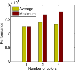
(a) Blogs: Offline results

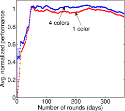
(b) Blogs: Online results

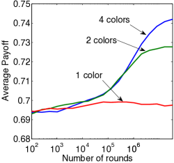
(c) Ad display: Online results

Figure 1: (a,b) Results for discounted blog ranking ($\gamma=0.8$), in offline (a) and online (b) setting. (c) Performance of TGonline with $C=1$, $2$, and $4$ colors for the sponsored search ad selection problem (each round is a query). Note that $C=1$ corresponds to the online algorithm of Radlinski et al. (2008) and Streeter and Golovin (2008).

6.2 Online ad display

We evaluate TGonline for the sponsored search ad selection problem in a simple Markovian model incorporating the value of diverse results and complex position-dependence among clicks. In this model, each user $u$ is defined by two sets of probabilities: $p_{\text{click}}(a)$ for each ad $a\in\mathcal{A}$, and $p_{\text{abandon}}(k)$ for each position $k\in\left[K\right]$. When presented an assignment of ads $\left\{a_{1},a_{2},\ldots,a_{K}\right\}$, where $a_{k}$ occupies position $k$, the user scans the positions in increasing order. For each position $k$, the user clicks on $a_{k}$ with probability $p_{\text{click}}(a_{k})$, leaving the results page forever. Otherwise, with probability $(1-p_{\text{click}}(a_{k}))\cdot p_{\text{abandon}}(k)$, the user loses interest and abandons the results without clicking on anything. Finally, with probability $(1-p_{\text{click}}(a_{k}))\cdot(1-p_{\text{abandon}}(k))$, the user proceeds to look at position $k+1$. The reward function $f_{t}$ is the number of clicks, which is either zero or one. We only receive information about $f_{t}(S_{t})$ (i.e., bandit feedback).

In our evaluation, there are $5$ positions, $20$ available ads, and two (equally frequent) types of users: type $1$ users interested in all positions ($p_{\text{abandon}}\equiv 0$), and type $2$ users that quickly lose interest ($p_{\text{abandon}}\equiv 0.5$). There are also two types of ads, half of type $1$ and half of type $2$, and users are probabilistically more interested in ads of their own type than those of the opposite type. Specifically, for both types of users we set $p_{\text{click}}(a)=0.5$ if $a$ has the same type as the user, and $p_{\text{click}}(a)=0.2$ otherwise. In Fig. 1(c) we compare the performance of TGonline with $C=4$ to the online algorithm of Radlinski et al. (2008); Streeter and Golovin (2008), based on the average of $100$ experiments. The latter algorithm is equivalent to running TGonline with $C=1$. They perform similarly in the first $10^{4}$ rounds; thereafter the former algorithm dominates.

It can be shown that with several different types of users with distinct $p_{\text{click}}(\cdot)$ functions the offline problem of finding an assignment within $1-\frac{1}{e}+\varepsilon$ of optimal is NP-hard. This is in contrast to the case in which $p_{\text{click}}$ and $p_{\text{abandon}}$ are the same for all users; in this case the offline problem simply requires finding an optimal policy for a Markov decision process, which can be done efficiently using well-known algorithms. A slightly different Markov model of user behavior which is efficiently solvable was considered in Aggarwal et al. (2008). In that model, $p_{\text{click}}$ and $p_{\text{abandon}}$ are the same for all users, and $p_{\text{abandon}}$ is a function of the ad in the slot currently being scanned rather than its index.

7 Related Work

An earlier version of this work appeared as Streeter et al. (2009) (also Golovin et al. (2009)). The present article is significantly extended, including a new algorithm for online optimization over arbitrary matroids. For a general introduction to the literature on submodular function maximization (including offline versions of the problems we study), see Vondrák (2007) and the survey by Krause and Golovin (2014). For an overview of applications of submodularity to machine learning and artificial intelligence, see Krause and Guestrin (2011).

In the online setting, the most closely related work is that of Streeter and Golovin (2008). Like us, they consider sequences of monotone submodular reward functions that arrive online, and develop an online algorithm that uses multi-armed bandit algorithms as subroutines. The key difference from our work is that, as in Radlinski et al. (2008), they are concerned with selecting a set of $K$ items rather than the more general problem of selecting an assignment of items to positions addressed in this paper. Kakade et al. (2007) considered the general problem of using $\alpha$-approximation algorithms to construct no $\alpha$-regret online algorithms, and essentially proved it could be done for the class of linear optimization problems in which the cost function has the form $c(S,w)$ for a solution $S$ and weight vector $w$, and $c(S,w)$ is linear in $w$. However, their result is orthogonal to ours, because our objective function is submodular and not linear.

Since the earlier version of this paper appeared, subsequent research has produced algorithms that incorporate context into their decisions: Dey et al. (2013) developed an algorithm for contextual optimization of sequences of actions, and used it to optimize control libraries used for various robotic planning tasks. Ross et al. (2013) developed an improved variant, and applied it to tasks such as news recommendation and document summarization.

8 Conclusions

In this paper, we showed that important problems, such as ad display in sponsored search and computing diverse rankings of information sources on the web, require optimizing assignments under submodular utility functions. We developed an efficient algorithm, TabularGreedy, which obtains the optimal approximation ratio of $(1-1/e)$ for this NP-hard optimization problem. We also developed an online algorithm, TGonline, that asymptotically achieves no $(1-1/e)$-regret for the problem of repeatedly selecting informative assignments, under the full-information and bandit-feedback settings. We demonstrated that our algorithm outperforms previous work on two real world problems, namely online ranking of informative blogs and ad allocation. Finally, we developed OnlineContinuousGreedy, an online algorithm that can handle more general matroid constraints, while still guaranteeing no $(1-1/e)$-regret.

Acknowledgments.

This work was supported in part by Microsoft Corporation through a gift as well as through the Center for Computational Thinking at Carnegie Mellon, by NSF ITR grant CCR-0122581 (The Aladdin Center), NSF grant IIS-0953413, and by ONR grant N00014-09-1-1044.

Appendix A: Proofs

Lemma 1 is a corollary of the following more general lemma. The difference between the two lemmas is that, unlike Lemma 1, Lemma 12 allows for the possibility that each $\mathop{\rm arg\,max}$ in the locally greedy algorithm is evaluated with additive error. We will need this result in analyzing TGonline later on.

Lemma 12

Let $f:\mathcal{P}\to\mathbb{R}_{\geq 0}$ be a function of the form $f(S)=f_{0}(S)+\sum_{k=1}^{K}f_{k}(S\cap P_{k})$, where $f_{0}:2^{\mathcal{V}}\to\mathbb{R}_{\geq 0}$ is monotone submodular, and $f_{k}:P_{k}\to\mathbb{R}_{\geq 0}$ is arbitrary for $k\geq 1$. Let $L=\left\{\ell_{1},\ell_{2},\ldots,\ell_{K}\right\}$, where $\ell_{k}\in P_{k}$ (for $1\leq k\leq K$). Suppose that for any $k$,

$$f(\left\{\ell_{1},\ell_{2},\ldots,\ell_{k}\right\})\geq\max_{x\in P_{k}}\left\{f(\left\{\ell_{1},\ell_{2},\ldots,\ell_{k-1}\right\}+x)\right\}-\varepsilon_{k}\mbox{ .}$$ (14)

Then

$$f(L)+f_{0}(L)\geq\max_{S\in\mathcal{P}}\left\{f(S)\right\}-\sum_{k=1}^{K}\varepsilon_{k}\mbox{ .}$$

Proof  Let $\textsf{OPT}=\mathop{\rm arg\,max}_{S\in\mathcal{P}}\left\{f(S)\right\}$, and let $\textsf{OPT}=\left\{o_{1},o_{2},\ldots,o_{K}\right\}$, where $o_{k}\in P_{k}$ (for $1\leq k\leq K$). Define

$$\Delta_{k}(L):=f_{k}(\left\{o_{k}\right\})+f_{0}(L\cup\left\{o_{1},o_{2},\ldots,o_{k}\right\})-f_{0}(L\cup\left\{o_{1},o_{2},\ldots,o_{k-1}\right\})\mbox{ .}$$

Let $L_{k}=\left\{\ell_{1},\ell_{2},\ldots,\ell_{k-1}\right\}$. Using submodularity of $f_{0}$, we have

$$\Delta_{k}(L) \leq f_{k}(\left\{o_{k}\right\})+f_{0}(L_{k}+o_{k})-f_{0}(L_{k})$$

$$=f(L_{k}+o_{k})-f(L_{k})$$

$$\leq f(L_{k}+\ell_{k})-f(L_{k})+\varepsilon_{k}\mbox{ .}$$

Then, using monotonicity of $f_{0}$,

$$f(\textsf{OPT}) \leq f_{0}(L\cup\textsf{OPT})+\sum_{k=1}^{K}f_{k}(\textsf{OPT}\cap P_{k})$$

$$=f_{0}(L)+\sum_{k=1}^{K}\Delta_{k}(L)$$

$$\leq f_{0}(L)+\sum_{k=1}^{K}f(L_{k}+\ell_{k})-f(L_{k})+\varepsilon_{k}$$

$$=f_{0}(L)+f(L)-f(\emptyset)+\sum_{k=1}^{K}\varepsilon_{k}\mbox{ .}$$

Rearranging this inequality and using $f(\emptyset)\geq 0$ completes the proof.  

To analyze TGonline, we will also need Theorem 13, which is a generalization of Theorem 2.

Theorem 13

Suppose $f$ is monotone submodular. Let $G=\left\{g_{k,c}:k\in\left[K\right],c\in\left[C\right]\right\}$, where $g_{k,c}\in P_{k}$ for all $k$ and $c$. Suppose that for all $k\in\left[K\right]$ and $c\in\left[C\right]$,

$$F(G^{-}_{k,c}+g_{k,c})\geq\max_{x\in P_{k}\times\left\{c\right\}}\left\{G^{-}_{k,c}+x\right\}-\varepsilon_{k,c}$$ (15)

where $G^{-}_{k,c}=\left\{g_{k^{\prime},c^{\prime}}:k^{\prime}\in\left[K\right],c^{\prime}<c\right\}\cup\left\{g_{k^{\prime},c}:k^{\prime}<k\right\}$ (i.e., $G^{-}_{k,c}$ equals $G$ just before $g_{k,c}$ is added). Then $f(G)\geq\beta(C,K)\cdot\max_{S\in\mathcal{P}}\left\{f(S)\right\}-\sum_{k=1}^{K}\sum_{c=1}^{C}\varepsilon_{k,c}$, where $\beta(C,K)$ is defined as $1-(1-\frac{1}{C})^{C}-{K\choose 2}C^{-1}$.

Proof  The proof is identical to the proof of Theorem 2 in the main text, using Lemma 12 in place of Lemma 1.  

Finally, we prove Theorem 5, which we restate here for convenience.

Theorem 5 Let $r_{k,c}$ be the regret of $\mathcal{E}_{k,c}$, and let $\beta(K,C)=1-\left({1-\frac{1}{C}}\right)^{C}-{K\choose 2}C^{-1}$. Then

$$\mathbb{E}\left[\sum_{t=1}^{T}f_{t}(G_{t})\right]\geq\beta(K,C)\cdot\max_{S\in\mathcal{P}}\left\{\sum_{t=1}^{T}f_{t}(S)\right\}-\mathbb{E}\left[\sum_{k=1}^{K}\sum_{c=1}^{C}r_{k,c}\right]\mbox{ .}$$

Proof  The idea of the proof is to view TGonline as a version of TabularGreedy that, instead of greedily selecting single (element,color) pairs $g_{k,c}\in P_{k}\times\left\{c\right\}$, greedily selects (element vector, color) pairs $\vec{g}_{k,c}\in P_{k}^{T}\times\left\{c\right\}$, where $T$ is the number of rounds.

First note that for any $k\in\left[K\right]$, $c\in\left[C\right]$, and $x\in P_{k}\times\left\{c\right\}$, by definition of $r_{k,c}$ we have

$$\sum_{t=1}^{T}\bar{F}_{t}\left({G^{t}_{k,c}+g^{t}_{k,c}}\right)\geq\left({\sum_{t=1}^{T}\bar{F}_{t}\left({G^{t}_{k,c}+x}\right)}\right)-r_{k,c}\mbox{ .}$$

Taking the expectation of both sides over $c$, and choosing $x$ to maximize the right hand side, we get

$$\sum_{t=1}^{T}F_{t}\left({G^{t}_{k,c}+g^{t}_{k,c}}\right)\geq\max_{x\in P_{k}\times\left\{c\right\}}\left\{\sum_{t=1}^{T}F_{t}\left({G^{t}_{k,c}+x}\right)\right\}-\varepsilon_{k,c}$$ (16)

where we define $F_{t}(S)=\mathbb{E}_{\vec{c}}\left[f_{t}(\textsf{sample}_{\vec{c}}(S))\right]$ and $\varepsilon_{k,c}=\mathbb{E}\left[r_{k,c}\right]$.

We now define some additional notation. For any set $\vec{S}$ of vectors in ${\mathcal{V}}^{T}$, define

$$f(\vec{S})=\sum_{t=1}^{T}f_{t}\left({\left\{\vec{a}_{t}:\vec{a}\in\vec{S}\right\}}\right)\mbox{ .}$$

Next, for any set $\vec{S}$ of (element vector, color) pairs in $\bigcup_{k=1}^{K}(P_{k}^{T}\times\left\{c\right\})$, define $\textsf{sample}_{\vec{c}}(\vec{S})=\bigcup_{k=1}^{K}\left\{\vec{x}\in P_{k}^{T}:(\vec{x},c_{k})\in\vec{S}\right\}$. Define $F(\vec{S})=\mathbb{E}_{\vec{c}}\left[f(\textsf{sample}_{\vec{c}}(\vec{S}))\right]$. By linearity of expectation,

$$F(\vec{S})=\sum_{t=1}^{T}F_{t}\left({\left\{(\vec{x}_{t},c):(\vec{x},c)\in\vec{S}\right\}}\right)\mbox{ .}$$ (17)

Let $\vec{g}_{k,c}=(\vec{x},c)$, where $\vec{x}$ is such that $(\vec{x}_{t},c)=g^{t}_{k,c}$ for all $t\in\left[T\right]$. Analogously to $G^{t-}_{k,c}$, define $\vec{G}^{-}_{k,c}=\left\{\vec{g}_{k^{\prime},c^{\prime}}:k^{\prime}\in\left[K\right],c^{\prime}<c\right\}\cup\left\{\vec{g}_{k^{\prime},c}:k^{\prime}<k\right\}$. By (17), for any $(\vec{x},c)\in{\mathcal{V}}^{T}\times\left[C\right]$ we have $F(\vec{G}^{-}_{k,c}+(\vec{x},c))=\sum_{t=1}^{T}F_{t}(G^{t-}_{k,c}+(\vec{x}_{t},c))$. Combining this with (16), we get

$$F\left({\vec{G}^{-}_{k,c}+\vec{g}_{k,c}}\right)\geq\max_{a:a\in P_{k}}\left\{F\left({\vec{G}^{-}_{k,c}+(a^{T},c)}\right)\right\}-\varepsilon_{k,c}$$ (18)

where $a^{T}$ is the unique element of $\left\{a\right\}^{T}$. Having proved (18), we can now use Theorem 13 to complete the proof. Let $\vec{P}_{k}:=\left\{a^{T}:a\in P_{k}\right\}$ for each $k\in\left[K\right]$, and define a new partition matroid over ground set $\left\{a^{T}:a\in{\mathcal{V}}\right\}$ with feasible solutions $\vec{\mathcal{P}}:=\left\{\vec{S}:\forall k\in\left[K\right],|\vec{S}\cap\vec{}P_{k}|\leq 1\right\}$. Let $\vec{G}=\left\{\vec{g}_{k,c}:k\in\left[K\right],c\in\left[C\right]\right\}$. As argued in the proof of Lemma 3, $F_{t}$ is monotone submodular. Using this fact together with (17), it is straightforward to show that $F$ itself is monotone submodular. Thus by Theorem 13,

$$F(\vec{G})\geq\beta(C,K)\cdot\max_{\vec{S}\in\vec{\mathcal{P}}}\left\{f(\vec{S})\right\}-\sum_{k=1}^{K}\sum_{c=1}^{C}\varepsilon_{k,c}\mbox{ .}$$

To complete the proof, it suffices to show that $F(\vec{G})=\mathbb{E}\left[\sum_{t=1}^{T}f_{t}(G_{t})\right]$, and that $\max_{\vec{S}\in\vec{\mathcal{P}}}\left\{f(\vec{S})\right\}\geq\max_{S\in\mathcal{P}}\left\{\sum_{t=1}^{T}f_{t}(S)\right\}$. Both facts follow easily from the definitions.

References

• Aggarwal etΒ al. (2008) Gagan Aggarwal, Jon Feldman, S.Β Muthukrishnan, and Martin PΓ‘l. Sponsored search auctions with Markovian users. In WINE, pages 621–628, 2008.
• Auer etΒ al. (2002) Peter Auer, NicolΓ² Cesa-Bianchi, Yoav Freund, and RobertΒ E. Schapire. The nonstochastic multiarmed bandit problem. SIAM Journal on Computing, 32(1):48–77, 2002.
• Blum and Mansour (2007) Avrim Blum and Yishay Mansour. From external to internal regret. Journal of Machine Learning Research, 8:1307–1324, 2007.
• Calinescu etΒ al. (2011) Gruia Calinescu, Chandra Chekuri, Martin PΓ‘l, and Jan VondrΓ‘k. Maximizing a submodular set function subject to a matroid constraint. SIAM Journal on Computing, 40(6):1740–1766, 2011.
• Cesa-Bianchi etΒ al. (1997) NicolΓ² Cesa-Bianchi, Yoav Freund, David Haussler, DavidΒ P. Helmbold, RobertΒ E. Schapire, and ManfredΒ K. Warmuth. How to use expert advice. J. ACM, 44(3):427–485, 1997.
• Dey etΒ al. (2013) Debadeepta Dey, TianΒ Yu Liu, Martial Hebert, and JΒ Andrew Bagnell. Contextual sequence prediction with application to control library optimization. Robotics, pageΒ 49, 2013.
• Edelman etΒ al. (2007) Benjamin Edelman, Michael Ostrovsky, and Michael Schwarz. Internet advertising and the generalized second price auction: Selling billions of dollars worth of keywords. American Economic Review, 97(1):242–259, 2007.
• Feldman and Muthukrishnan (2008) Jon Feldman and S.Β Muthukrishnan. Algorithmic methods for sponsored search advertising. In Zhen Liu and CathyΒ H. Xia, editors, Performance Modeling and Engineering. 2008. doi: 10.1007/978-0-387-79361-0β€œΛ™4. URL http://dx.doi.org/10.1007/978-0-387-79361-0_4.
• Fisher etΒ al. (1978) MarshallΒ L. Fisher, GeorgeΒ L. Nemhauser, and LaurenceΒ A. Wolsey. An analysis of approximations for maximizing submodular set functions - II. Mathematical Programming Study, (8):73–87, 1978.
• Golovin etΒ al. (2009) Daniel Golovin, Andreas Krause, and Matthew Streeter. Online learning of assignments that maximize submodular functions. CoRR, abs/0908.0772, 2009.
• Kakade etΒ al. (2007) ShamΒ M. Kakade, AdamΒ Tauman Kalai, and Katrina Ligett. Playing games with approximation algorithms. In STOC, pages 546–555, 2007.
• Kalai and Vempala (2005) Adam Kalai and Santosh Vempala. Efficient algorithms for online decision problems. Journal of Computer and System Sciences, 71(3):291–307, 2005. ISSN 0022-0000. doi: http://dx.doi.org/10.1016/j.jcss.2004.10.016.
• Krause and Golovin (2014) Andreas Krause and Daniel Golovin. Submodular function maximization. In Tractability: Practical Approaches to Hard Problems (to appear). Cambridge University Press, February 2014. URL files/krause12survey.pdf.
• Krause and Guestrin (2011) Andreas Krause and Carlos Guestrin. Submodularity and its applications in optimized information gathering. ACM Transactions on Intelligent Systems and Technology, 2(4), July 2011. URL http://dl.acm.org/citation.cfm?id=1989736.
• Lahaie etΒ al. (2007) SΓ©bastien Lahaie, DavidΒ M. Pennock, Amin Saberi, and RakeshΒ V. Vohra. Sponsored search auctions. In Noam Nisan, Tim Roughgarden, Eva Tardos, and VijayΒ V. Vazirani, editors, Algorithmic Game Theory. Cambridge University Press, New York, NY, USA, 2007. ISBN 0521872820.
• Leskovec etΒ al. (2007) Jure Leskovec, Andreas Krause, Carlos Guestrin, Christos Faloutsos, Jeanne VanBriesen, and Natalie Glance. Cost-effective outbreak detection in networks. In KDD, pages 420–429, 2007.
• Mirrokni etΒ al. (2008) Vahab Mirrokni, Michael Schapira, and Jan VondrΓ‘k. Tight information-theoretic lower bounds for welfare maximization in combinatorial auctions. In EC, pages 70–77, 2008.
• Nemhauser etΒ al. (1978) GeorgeΒ L. Nemhauser, LaurenceΒ A. Wolsey, and MarshallΒ L. Fisher. An analysis of approximations for maximizing submodular set functions - I. Mathematical Programming, 14(1):265–294, 1978.
• Radlinski etΒ al. (2008) Filip Radlinski, Robert Kleinberg, and Thorsten Joachims. Learning diverse rankings with multi-armed bandits. In ICML, pages 784–791, 2008.
• Ross etΒ al. (2013) Stephane Ross, Jiaji Zhou, Yisong Yue, Debadeepta Dey, and Drew Bagnell. Learning policies for contextual submodular prediction. In Proceedings of The 30th International Conference on Machine Learning, pages 1364–1372, 2013.
• Schrijver (2003) Alexander Schrijver. Combinatorial optimization : polyhedra and efficiency. Volume B: Matroids, Trees, Stable Sets, chapters 39-69. Springer, 2003.