Abstract

In this work we study the radiative corrections to the mass of the lightest Higgs boson of the MSSM from three generations of Majorana neutrinos and sneutrinos. The spectrum of the MSSM is augmented by three right handed neutrinos and their supersymmetric partners. A seesaw mechanism of type I is used to generate the physical neutrino masses and oscillations that we require to be in agreement with present neutrino data. We present a full one-loop computation of these Higgs mass corrections, and analyze in full detail their numerical size in terms of both the MSSM and the new (s)neutrino parameters. A critical discussion on the different possible renormalization schemes and their implications, in particular concerning decoupling, is included.

1 Introduction

In order to account for the impressive experimental data on neutrino mass differences and neutrino mixing angles [1] physics beyond the Standard Model (SM) is needed. On the other hand, after the discovery of a Higgs boson at the Large Hadron Collider (LHC) [2, 3], the problem of stabilizing the Higgs mass at the electroweak scale within the SM became even more relevant. Similarly, the existence of Cold Dark Matter (CDM) [4] has to be accounted for by an extension of the SM. Consequently, in order to incorporate neutrino masses into the SM, to stabilize the Higgs-boson mass scale and to provide a viable CDM we choose here one of the most popular extensions of the SM: the simplest version of a supersymmetric extension of the SM, the Minimal Supersymmetric Standard Model (MSSM) [5, 6, 7], with the addition of heavy right-handed Majorana neutrinos, and where the well known seesaw mechanism of type I [8, 9, 10, 11, 12, 13] is implemented to generate the observed small neutrino masses. From now on we will denote this model by “MSSM-seesaw”. The lightest Higgs boson in this model can be interpreted as the Higgs particle discovered at the LHC [14].

In this MSSM-seesaw context, the smallness of the light neutrino masses, $m_{\nu}\sim m_{D}^{2}/m_{M}$, appears naturally due to the induced large suppression by the ratio of the two very distant mass scales. Namely, the Majorana neutrino mass $m_{M}$, that represents the new physics scale, and the Dirac neutrino mass $m_{D}$, which is related to the electroweak scale via the neutrino Yukawa couplings $Y_{\nu}$, by $m_{D}=Y_{\nu}v\sin\beta$. The Higgs sector content in the MSSM-seesaw is as in the MSSM, i.e. composed of two Higgs doublets. $\tan\beta$ is the ratio of the two vacuum expectation values, $\tan\beta=v_{2}/v_{1}$, and $v^{2}=v_{1}^{2}+v_{2}^{2}=(174\,\,\mathrm{GeV})^{2}$. Small neutrino masses of the order of $m_{\nu}\sim\mathcal{O}(0.1)$ eV can be easily accommodated with large Yukawa couplings, $Y_{\nu}\sim{\cal O}(1)$, if the new physics scale is very large, within the range $m_{M}\sim 10^{13}-10^{15}\,\,\mathrm{GeV}$. This is to be compared with the Dirac neutrino case where, in order to get similar small neutrino masses, extremely tiny, hence irrelevant, Yukawa couplings of the order of $Y_{\nu}\sim 10^{-12}-10^{-13}$ are required.

As for all SM fermions, the neutrinos in the MSSM are accompanied by their respective super partners, the scalar neutrinos. The hypothesis of Majorana massive (s)neutrinos is very appealing for various reasons, including the interesting possibility of generating satisfactorily baryogenesis via leptogenesis [15]. Furthermore, they can produce an interesting phenomenology due to their potentially large Yukawa couplings to the Higgs sector of the MSSM, such as corrections to the light ${\cal CP}$-even Higgs-boson mass, $M_{h}$ [16, 17] (see also  [18, 19, 20, 21] for previous evaluations). Further striking phenomenological implications [22] of the MSSM-seesaw scenario are the prediction of sizeable rates for lepton flavor violating processes (within the present experimental reach for specific areas of the model parameters [23, 24, 25, 26, 27, 28, 29, 30, 31]), non-negligible contributions to electric dipole moments of charged leptons [32, 33, 34], and also the occurrence of sneutrino-antisneutrino oscillations [35] as well as sneutrino flavor-oscillations [36].

It is worth recalling that the seesaw mechanism is not the only way to generate neutrino masses in the context of supersymmetry (see, for instance, [37, 38]). In fact there are many well known extensions of the MSSM that can generate small neutrino masses besides the various types of high and low scale Seesaw models (see e.g,[39] for a review and references therein). One possible alternative to the addition of right-handed neutrinos is the incorporation of R-parity violating interactions to the MSSM, which can introduce the lepton number violating terms that are needed for the small neutrino mass generation. Indeed, R-parity violation can be produced in many ways: spontaneously, explicitly, by bi-linear terms, by trilinear terms, etc., see, e.g, ref.[40, 41]. Another popular extension of the MSSM is the Next-to-Minimal-Supersymmetric-Standard-Model (NMSSM) (see, for instance, the review in [42]), which includes an extra chiral singlet superfield with zero lepton number, offering a solution to the so-called $\mu$-problem of the MSSM and providing an extra tree level mass term to the SM-like Higgs boson which raises its mass above that of the lightest Higgs boson of the MSSM. In this NMSSM, as in the MSSM, the small neutrino masses can be generated either by allowing for R-parity violating terms or by adding extra chiral singlet superfields carrying non-vanishing lepton number (like, for instance, right-handed neutrinos). The $\mu\nu$SSM [43] can also solve the $\mu$ problem and generate masses for the neutrinos by adding to the MSSM right-handed neutrino superfields and R-parity breaking terms.

It should be noted that each of the above mentioned extensions of the MSSM leads to different phenomenological implications, including those in the neutrino and in the Higgs boson sectors. Our preference for the particular choice of extended MSSM with three generations of right handed neutrinos and sneutrinos, and with a seesaw mechanism of type I, is mainly because, as we have said above, it is the simplest extension of the MSSM compatible with neutrino data that naturally allows for large neutrino Yukawa couplings. It is precisely this interesting possibility of large neutrino Yukawa couplings what can induce large radiative corrections to the lightest Higgs boson mass, and thus the (s)neutrino sector phenomenology is directly linked to the Higgs sector. Other extensions of the MSSM could also induce relevant corrections to the Higgs boson mass from the additional superfields and the new input parameters associated to the neutrino mass generation. For instance, within the NMSSM, in addition to the tree level enhanced Higgs boson mass, one may generate relevant mass corrections from the TeV-scale right-handed neutrinos via their interactions with the zero-lepton-number chiral singlet superfield while having small neutrino Yukawa couplings[44]. Alternatively, one may also generate relevant corrections to the Higgs boson mass from TeV-scale right-handed neutrinos, within the context of the Inverse Seesaw Models, that allow for large Yukawa couplings but introduce in addition a small lepton number violating parameter[45].

We are interested here in the indirect effects of Majorana neutrinos and sneutrinos via their radiative corrections to the MSSM Higgs boson masses within the MSSM-seesaw framework. While the initial evaluations and analyses of corrections to $M_{h}$ concentrated on the one-generation case to analyze the general analytic behavior of this type of contributions, in this paper we investigate the Majorana neutrino and sneutrino sectors with three generations which can accommodate the present neutrino data. We will focus here on the corrections to the lightest $M_{h}$ and will present the full one-loop contributions from the complete three generations of neutrinos and sneutrinos and without using any approximation. It should be noted that the extrapolation from the one generation to the three generations case cannot be trivially done due to the relevant generation mixing in the latter and, therefore, the corresponding radiative corrections must be explicitly and separately computed. A crucial issue of interest in relation with the present computation is the question of decoupling of the heavy Majorana mass scales. While it was shown for the one generation case [16, 17] that this strongly depends on the choice of the renormalization scheme, no such scheme could be identified being superior to the other in all respects. Consequently, we will also comment comparatively the advantages and disadvantages of the various renormalization schemes in the present case of three generations where there are several mass scales involved. On the one hand it will not be possible to obtain information from a precise $M_{h}$ measurement on the Majorana mass scale. On the other hand, however, the precise prediction of $M_{h}$ in the presence of Majorana (s)neutrinos and the understanding of these corrections in the different schemes (and their respective decoupling behavior) used in the $M_{h}$ calculations, is desirable.

For the estimates of the total corrections to $M_{h}$ in the MSSM-seesaw, obviously, the one-loop corrections from the neutrino/sneutrino sector that we are interested here have to be added to the existing MSSM corrections. The status of radiative corrections to $M_{h}$ in the non-$\nu/\tilde{\nu}$ sector, i.e. in the MSSM without massive neutrinos, can be summarized as follows. Full one-loop calculations [46, 47, 48] have been supplemented by the leading and subleading two-loop corrections, see [49] and references therein. Together with leading three-loop corrections [50, 51, 52] and the recently added resummation of logarithmic contributions [53], the current precision in $M_{h}$ is estimated to be $\sim 2-3\,\,\mathrm{GeV}$ [49, 53, 54].

A summary and discussion of the previous estimates of neutrino/sneutrino radiative corrections to the Higgs mass parameters can be found in [16], where (as discussed above) the one-generation case was calculated and analyzed. In this work, we will consider the more general three generation MSSM-seesaw scenarios with no universality conditions imposed, and explore the full parameter space, without restricting ourselves just to large or small values of any of the relevant neutrino/sneutrino parameters. In principle, since the right handed Majorana neutrinos and their SUSY partners are $SU(2)\times U(1)$ singlets, there is no a priori reason why the size of their associated parameters should be related to the size of the other sector parameters. In the numerical estimates, we will therefore explore a wide interval for all the involved neutrino/sneutrino relevant input parameters.

The paper is organized as follows. In Sect. 2, we summarize the most important ingredients of the MSSM-seesaw scenario that are needed for the present computation of the Higgs mass loop corrections. These include, the setting of the model parameters and the complete list of the Lagrangian relevant terms. A complete set of the corresponding relevant Feynman rules in the physical basis is also provided here. They are collected in App. A (to our knowledge, they are not available in the previous literature). In Sect. 3 we discuss the renormalization procedure and emphasize the differences between the selected renormalization schemes. The corresponding analytic analysis can be found in Sect. 4. A numerical evaluation and in particular the dependence on the (hierarchical) Majorana mass scales is given in Sect. 5. Finally, our conclusions can be found in Sect. 6.

2 The MSSM-seesaw model

In order to include the proper neutrino masses and oscillations in agreement with present neutrino data (see, for instance, [55, 56, 57]), we employ an extended version of the MSSM, where three right handed neutrinos and their supersymmetric partners are included, in addition to the usual MSSM spectra. A seesaw mechanism of type I [8, 9, 10, 11, 12, 13] is implemented which requires in addition to the Dirac neutrino mass matrix, $m_{D}$, the introduction of a new $3\times 3$ so-called Majorana mass matrix, $m_{M}$. This matrix $m_{M}$ is the responsible for the Majorana character of the physical neutrinos in this MSSM-seesaw model.

The terms of the superpotential within the MSSM-seesaw that are relevant for neutrino and Higgs related physics are described by [16, 35, 36]:

$$W\,=\,\epsilon_{ab}\left[Y_{\nu}^{ij}\hat{\mathcal{H}}_{2}^{a}\,\hat{L}_{i}^{b}\hat{N}_{j}\,-\,Y_{l}^{ij}\hat{\mathcal{H}}_{1}^{a}\,\hat{L}_{i}^{b}\,\hat{R}_{j}\,+\,\mu\hat{\mathcal{H}}_{1}^{a}\hat{\mathcal{H}}_{2}^{b}\right]\,+\,\dfrac{1}{2}\,m_{M}^{ij}\,\hat{N}_{i}\,\hat{N}_{j}\,.$$ (1)

$Y_{\nu}$ is a $3\times 3$ complex Yukawa matrix, while $m_{M}$ is a complex symmetric $3\times 3$ mass matrix. The indices $i,\,j$ represent generations (with $i,\,j=1,2,3$), the indices $a,\,b$ refer to $SU(2)$ doublets components, and $\epsilon_{12}=-1$. Omitting the generation indexes, for brevity, the involved superfields are as follows: $\hat{N}=\{\tilde{\nu}_{R}^{*},(\nu_{R})^{c}\}$ is the new superfield that contains the right-handed neutrinos $\nu_{R_{i}}$ and their partners $\tilde{\nu}_{R_{i}}$, while the other superfields are as in the MSSM, i.e., $\hat{L}$ contains the $SU(2)$ lepton doublet, $(\nu_{L},l_{L})$ and its superpartner $(\tilde{\nu}_{L},\tilde{l}_{L})$, $\hat{R}$ contains the $SU(2)$ sfermion and fermion singlets $\{\tilde{l}_{R},(l_{R})^{c}\}$, and the $\mathcal{\hat{H}}_{1}$ and $\hat{\mathcal{H}}_{2}$ are the Higgs superfields that give masses to the down and up-type (s)fermions, respectively. Here and in the following, $f^{c}$ refers to the particle-antiparticle conjugate of a fermion $f$ defined as follows:

$$\hat{C}:f\rightarrow f^{c} =C\left.\bar{f}^{T}\right.\,,$$ (2)

where $\hat{C}$ and $C$ are the particle-antiparticle conjugation and charge conjugation respectively.

The superfields $\hat{L},\hat{N}$ and $\hat{R}$ can be chosen such that $Y_{l}$ and $m_{M}$ are real and non-negative diagonal $3\times 3$ matrices, whereas $Y_{\nu}$, in contrast, is a general complex $3\times 3$ matrix.

The additional sneutrinos $\tilde{\nu}_{R_{i}}$ induce new relevant terms in the soft SUSY-breaking potential. Following [16, 35, 36] it can be written as:

$$V^{\tilde{\nu}}_{\text{soft}}=\left(m^{2}_{\tilde{L}}\right)^{ij}\tilde{\nu}_{L_{i}}^{*}\tilde{\nu}_{L_{j}}+\left(m^{2}_{\tilde{R}}\right)^{ij}\tilde{\nu}_{R_{i}}\tilde{\nu}_{R_{j}}^{*}+\left(A_{\nu}^{ij}H^{2}_{2}\tilde{\nu}_{L_{i}}\tilde{\nu}_{R_{j}}^{*}+\left(m_{B}^{2}\right)^{ij}\tilde{\nu}_{R_{i}}^{*}\tilde{\nu}_{R_{j}}^{*}+{\text{h.c.}}\right),$$ (3)

where $m^{2}_{\tilde{L}}$, $m^{2}_{\tilde{R}}$ are $3\times 3$ hermitian matrices in the flavor space, $A_{\nu}$ is a $3\times 3$ generic complex matrix and $m_{B}^{2}$ is a complex symmetric matrix.

After the Higgs fields develop a vacuum expectation value, the charged lepton and Dirac neutrino mass matrix elements can be written as:

$$m_{l}^{ij}\, = \,Y_{l}^{ij}\,\,v_{1}\,,$$

$$m_{D}^{ij}\, = \,Y_{\nu}^{ij}\,v_{2}\,,$$ (4)

where $v_{i}$ are the vacuum expectation values (vev) of the $H_{i}$ fields, $v_{1}=v\cos\beta$, $v_{2}=v\sin\beta$ and $v^{2}=\dfrac{2M_{W}^{2}}{g^{2}}=\dfrac{2M_{Z}^{2}}{g^{2}+g^{\prime 2}}=(174\text{ GeV})^{2}$. $M_{W}$ and $M_{Z}$ denote the masses of the $W$ and $Z$ boson, respectively.

Finally, starting with the superpotential of (1), the Yukawa couplings of the neutrinos and their corresponding mass terms can be derived:

$$-{\mathcal{L}}_{\rm{mass}}-{\mathcal{L}}_{\rm{Yukawa}}=\dfrac{1}{2}\sum_{ij}\left[\dfrac{\partial^{2}W\left(\phi\right)}{\partial{\phi_{i}}\partial{\phi_{j}}}\psi_{i}\psi_{j}+\rm{h.c.}\right]\,,$$ (5)

where the $\psi_{i}$ are the two component fermion field superpartners of the corresponding scalar component $\phi_{i}$ of the super fields.

2.1 Neutrino mass and interaction Lagrangians

After the Higgs field develops a vacuum expectation value, the mass Lagrangian of neutrinos in the MSSM-seesaw model with three generations of $\nu_{L}$ and $\nu_{R}$ is given by:

$$-\mathcal{L}_{\text{mass}}^{\nu}=\overline{\nu_{R_{i}}}\,\,m_{D_{ij}}^{{\dagger}}\nu_{L_{j}}+\overline{\nu_{L_{i}}}\,\,m_{D_{ij}}\nu_{R_{j}}+\frac{1}{2}\overline{\left(\nu_{R_{i}}\right)^{c}}\,\,m_{M_{ij}}\nu_{R_{j}}+\frac{1}{2}\overline{\nu_{R_{i}}}\,m_{M_{ij}}^{{\dagger}}\left(\nu_{R_{j}}\right)^{c},$$ (6)

where we have used again the notation $i,j$ for generation indexes, and $m_{D}$ and $m_{M}$ are the Dirac and Majorana mass matrices, respectively, which have been introduced in the previous section (2).

Notice that the particle-antiparticle conjugation operator $\hat{C}$ flips the chirality of a particle and changes all the quantum numbers of it. Then, it changes a left handed neutrino by a right handed antineutrino and a right handed neutrino by a left handed antineutrino. Following (2):

$$\hat{C}:\,\,\nu_{L}\to\left(\nu_{L}\right)^{c}=\left(\nu^{c}\right)_{R}\,,$$

$$\hat{C}:\,\,\nu_{R}\to\left(\nu_{R}\right)^{c}=\left(\nu^{c}\right)_{L}\,.$$ (7)

If a neutrino is a Majorana fermion it is invariant under $\hat{C}$. As a result, $\nu^{c}=\nu$.

The $\mathcal{L}_{\text{mass}}^{\nu}$ of (6) can be rewritten in a more compact form:

$$-\mathcal{L}^{\nu}_{\text{mass}}=\dfrac{1}{2}\left(\overline{\nu_{L}},\overline{\left(\nu_{R}\right)^{c}}\right)_{i}M^{\nu}_{ij}\left(\begin{array}[]{c}\left(\nu_{L}\right)^{c}\\ \nu_{R}\end{array}\right)_{j}+h.c.\,,$$ (8)

where

$$M^{\nu}=\left(\begin{array}[]{cc}0&m_{D}\\ m_{D}^{T}&m_{M}\end{array}\right)$$ (9)

is a $6\times 6$ complex symmetric matrix which can be diagonalized by an unitary matrix $U$:

$$U^{T}M^{\nu}U=\hat{M}^{\nu}=\text{diag}\left(m_{n_{1}},m_{n_{2}},m_{n_{3}},m_{n_{4}},m_{n_{5}},m_{n_{6}}\right)\,.$$ (10)

Here, the diagonal elements of $\hat{M}^{\nu}$, $m_{n_{i}}$, are the non negative square roots of the eigenvalues of $\left(M^{\nu}\right)^{\dagger}M^{\nu}$.

The interaction eigenstates are the left and right handed components of the neutrino fields, $\nu_{L_{i}}$ and $\nu_{R_{i}}$ (with $i=1,2,3$), and are related to the mass eigenstates $n_{j}$ (with $j=1,...,6$) in the following way:

$$\left(\nu_{L}\right)^{c}_{i} = U_{ij}P_{R}n_{j}\,,$$

$$\nu_{R_{i}} = U_{i+3,j}P_{R}n_{j}\,.$$ (11)

where here and from now on, we shorten the notation to $U_{ij}\equiv U_{i,j}$. Similarly for the $\hat{C}$-conjugate relations:

$$\nu_{L_{i}} = U_{ij}^{*}P_{L}n_{j}\,,$$

$$\left(\nu_{R}\right)^{c}_{i} = U_{i+3,j}^{*}P_{L}n_{j}\,.$$ (12)

In the seesaw limit, i.e. if $||m_{D}||\ll||m_{M}||$ , an analytic perturbative diagonalization in blocks can be performed by expanding in powers of the dimensionless parameter matrix $\xi=m_{D}m_{M}^{-1}$. This allows us to separate the light sector from the heavy sector by the introduction of a $6\times 6$ matrix:

$$\hat{U}^{\nu}\ =\ \left(\begin{array}[]{cc}(1-\frac{1}{2}\xi^{*}\xi^{T})&\xi^{*}(1-\frac{1}{2}\xi^{T}\xi^{*})\\ -\xi^{T}(1-\frac{1}{2}\xi^{*}\xi^{T})&(1-\frac{1}{2}\xi^{T}\xi^{*})\end{array}\right)+\mathcal{O}(\xi^{4})\,.$$ (13)

Two independent blocks of $3\times 3$ neutrino mass matrices are obtained once this $\hat{U}^{\nu}$ matrix is inserted in (10):

$$m_{\nu} = -m_{D}\xi^{T}+\mathcal{O}(m_{D}\xi^{3})\simeq-m_{D}m_{M}^{-1}m_{D}^{T}\,,$$ (14)

$$m_{N} = m_{M}+\mathcal{O}(m_{D}\xi)\simeq m_{M}\,.$$ (15)

The matrix $m_{N}$ of (15) is already diagonal and its diagonal elements $m_{N_{1}}$, $m_{N_{2}}$ and $m_{N_{3}}$ are approximately the three respective Majorana masses, $m_{M_{1}}$, $m_{M_{2}}$, $m_{M_{3}}$. The diagonalization of the matrix $m_{\nu}$ of (14) is performed as usual by the Pontecorvo-Maki-Nakagawa-Sakata (PMNS) unitary matrix [58, 59], $U_{\text{PMNS}}$ given by:

$$U_{\text{PMNS}}=\left(\begin{array}[]{ccc}c_{12}\,c_{13}&s_{12}\,c_{13}&s_{13}\,e^{-i\delta}\\ -s_{12}\,c_{23}\,-\,c_{12}\,s_{23}\,s_{13}\,e^{i\delta}&c_{12}\,c_{23}\,-\,s_{12}\,s_{23}\,s_{13}\,e^{i\delta}&s_{23}\,c_{13}\\ s_{12}\,s_{23}\,-\,c_{12}\,c_{23}\,s_{13}\,e^{i\delta}&-c_{12}\,s_{23}\,-\,s_{12}\,c_{23}\,s_{13}\,e^{i\delta}&c_{23}\,c_{13}\end{array}\right)\,\times\,V\,,$$ (16)

where

$$V=\text{diag}\,(e^{-i\phi_{1}/2},e^{-i\phi_{2}/2},1)\,,$$ (17)

and the notation $c_{ij}\equiv\cos\theta_{ij}$, $s_{ij}\equiv\sin\theta_{ij}$ has been used. Here, $\theta_{ij}$ are the mixing angles of the light neutrinos, $\delta$ is the Dirac phase and $\phi_{1,2}$ are the two Majorana phases.

As a result, the mass eigenvalues $m_{n_{j}}$, corresponding to light Majorana neutrinos $\left(\nu\right)$ and heavy Majorana neutrinos $\left(N\right)$ are given respectively by:

$$m_{\nu}^{\text{diag}} = U_{\text{PMNS}}^{T}m_{\nu}U_{\text{PMNS}}=\text{diag}\,(m_{\nu_{1}},m_{\nu_{2}},m_{\nu_{3}})\,,$$ (18)

$$m_{N}^{\text{diag}} = \text{diag}(m_{N_{1}},m_{N_{2}},m_{N_{3}})\simeq\text{diag}\,(m_{M_{1}},m_{M_{2}},m_{M_{3}})\,.$$ (19)

In this work, in order to make contact with the experimental data, we have used the Casas-Ibarra parametrization [60], which provides a simple way to reconstruct the Dirac mass matrix by using as inputs the physical light $m_{\nu_{i}}$ and heavy $m_{N_{i}}$ neutrino masses, the $U_{\text{PMNS}}$ matrix, and a general complex and orthogonal matrix $R$:

$$m_{D}^{T}=i\sqrt{m_{N}^{\text{diag}}}\,R\,\sqrt{m_{\nu}^{\text{diag}}}\,U_{\text{PMNS}}^{\dagger}\,,$$ (20)

where $R^{T}R=RR^{T}={\rm 1\kern-1.19995pt\rule{0.3pt}{6.45831pt}\raisebox{0.0pt}{\rule{1.00006pt}{0.3pt}}}$ and where we have considered the following parametrization:

$$R=\left(\begin{array}[]{ccc}c_{2}c_{3}&-c_{1}s_{3}-s_{1}s_{2}c_{3}&s_{1}s_{3}-c_{1}s_{2}c_{3}\\ c_{2}s_{3}&c_{1}c_{3}-s_{1}s_{2}s_{3}&-s_{1}c_{3}-c_{1}s_{2}s_{3}\\ s_{2}&s_{1}c_{2}&c_{1}c_{2}\end{array}\right)\,,$$ (21)

where $c_{i}\equiv\cos\theta_{i}$, $s_{i}\equiv\sin\theta_{i}$ and $\theta_{1}$, $\theta_{2}$ and $\theta_{3}$ are arbitrary complex angles.

Thus, our set of input values consist of $m_{M_{1}}$, $m_{M_{2}}$, $m_{M_{3}}$ and $\theta_{i}$, and for $m_{\nu_{1}}$, $m_{\nu_{2}}$, $m_{\nu_{3}}$ and $U_{\text{PMNS}}$ we use their suggested values from the experimental data are used. For the numerical estimates in this work we will use the following input values for the light neutrino mass squared differences and the angles in the $U_{\text{PMNS}}$ matrix:

$$\Delta m^{2}_{21}\,=7.50\times 10^{-5}{\rm eV}^{2}\,,\quad\quad|\Delta m^{2}_{32}|\,=2.42\times 10^{-3}{\rm eV}^{2}\,,$$

$$\sin^{2}{(2\theta_{12})}=0.857\,,\quad\sin^{2}{(2\theta_{23})}=0.95\,,\quad\sin^{2}{(2\theta_{13})}=0.098\,,\quad\quad\delta=\phi_{1}=\phi_{2}=0\,,$$ (22)

Notice that $\Delta m^{2}_{32}>0$ for light neutrinos with a normal hierarchy and $\Delta m^{2}_{32}<0$ for an inverted light neutrino hierarchy. These values are compatible with the present experimental data. Specifically, the recent global fit NuFIT 1.3 (2014) [56] sets:

$$\sin^{2}\theta_{12} =0.304^{+0.012}_{-0.012}\,, \Delta m^{2}_{21} =7.50^{+0.19}_{-0.17}\times 10^{-5}\;\mathrm{eV}^{2}\,,$$

$$\sin^{2}\theta_{23} =0.451^{+0.001}_{-0.001}\,, \Delta m^{2}_{31} =2.458^{+0.002}_{-0.002}\times 10^{-3}\;\mathrm{eV}^{2}\,({\rm NH}),$$ (23)

$$\sin^{2}\theta_{13} =0.0219^{+0.0010}_{-0.0011}\,, \Delta m^{2}_{32} =-2.448^{+0.047}_{-0.047}\times 10^{-3}\;\mathrm{eV}^{2}\,({\rm IH}),$$

where NH and IH refer to the normal hierarchy and inverted hierarchy cases for the light neutrinos, respectively.

The interaction Lagrangian of the MSSM neutral Higgs bosons with the three $\nu_{L}$ and three $\nu_{R}$ neutrinos is given, in compact form, by:

$$\mathcal{L}^{{\rm Higgs}}_{\nu_{L}\nu_{R}} = -\dfrac{g}{2M_{W}\sin\beta}\left(\overline{\nu_{R}}m_{D}^{\dagger}\nu_{L}+\overline{\nu_{L}}m_{D}\nu_{R}\right)\left(H\sin\alpha+h\cos\alpha\right)$$ (24)

$$-\dfrac{ig}{2M_{W}\sin\beta}\left(\overline{\nu_{R}}m_{D}^{\dagger}\nu_{L}-\overline{\nu_{L}}m_{D}\nu_{R}\right)A\cos\beta.$$

Here $\alpha$ is the angle that diagonalizes the ${\cal CP}$-even Higgs sector at the tree-level.

By using (2.1) and (2.1) the interaction Lagrangian in (24) can be expressed in terms of the neutrino mass eigenstates $n_{i}=(n_{1},\ldots,n_{6})$:

$$\mathcal{L}^{{\rm Higgs}}_{n_{j}n_{i}} = \dfrac{-g}{2M_{W}\sin\beta}\,\overline{n}_{j}\Big{[}U_{l+3,j}^{*}\left(m_{D}^{\dagger}\right)_{lm}U_{mi}^{*}P_{L}+U_{lj}\left(m_{D}\right)_{lm}U_{m+3,i}P_{R}\Big{]}n_{i}\left(H\sin\alpha+h\cos\alpha\right)$$ (25)

$$-\dfrac{ig}{2M_{W}\sin\beta}\,\overline{n}_{j}\Big{[}U_{l+3,j}^{*}\left(m_{D}^{\dagger}\right)_{lm}U_{mi}^{*}P_{L}-U_{lj}\left(m_{D}\right)_{lm}U_{m+3,i}P_{R}\Big{]}n_{i}\,A\cos\beta\,,$$

where $j$ and $i$ indexes run from 1 to 6 and $l$ and $m$ indexes run from 1 to 3.

The gauge interactions of $\nu_{L}$ (the $\nu_{R}$ have no interactions since they are singlets) with the neutral gauge boson $Z$ are given, in compact form, by:

$$\mathcal{L}_{\nu_{L}\nu_{L}}^{Z}=-\dfrac{g}{2c_{\mathrm{w}}}\left(\overline{\nu_{L}}\,\gamma^{\mu}\nu_{L}\right)Z_{\mu}\,.$$ (26)

When expressed in terms of the physical neutrino basis it gives:

$$\mathcal{L}_{n_{j}n_{i}}^{Z}=-\dfrac{g}{2c_{\mathrm{w}}}\left(\overline{n}_{j}U_{mj}U_{mi}^{*}\gamma^{\mu}P_{L}n_{i}\right)Z_{\mu}$$ (27)

where the indexes $i$ and $j$ run from 1 to 6 and $m$ runs from 1 to 3.

2.2 Sneutrino mass and interaction Lagrangians

Following [36], we will express the sneutrino mass terms in a compact $6\times 6$ matrix form by defining two six-dimensional vectors $\phi_{L}=(\tilde{\nu}_{L}\ \ \tilde{\nu}_{L}^{*})^{T}$ and $\phi_{N}=(\tilde{N}\ \ \tilde{N}^{*})^{T}=(\tilde{\nu}_{R}^{*}\ \ \tilde{\nu}_{R})^{T}$. In this new basis, the mass Lagrangian of the sneutrinos has the form:

$$-\mathcal{L}_{\rm mass}\,\, = \dfrac{1}{2}\left(\begin{array}[]{cc}\phi_{L}^{\dagger}&\phi_{N}^{\dagger}\end{array}\right)\left(\begin{array}[]{cc}M_{LL}^{2}&M_{LN}^{2}\\ \left(M_{LN}^{2}\right)^{\dagger}&M_{NN}^{2}\end{array}\right)\left(\begin{array}[]{c}\phi_{L}\\ \phi_{N}\end{array}\right)$$ (33)

$$= \dfrac{1}{2}\left(\begin{array}[]{cccc}\tilde{\nu}_{L}^{*T}&\tilde{\nu}_{L}^{T}&\tilde{\nu}_{R}^{T}&\tilde{\nu}_{R}^{*T}\end{array}\right)M_{\tilde{\nu}}^{2}\left(\begin{array}[]{c}\tilde{\nu}_{L}\\ \tilde{\nu}_{L}^{*}\\ \tilde{\nu}_{R}^{*}\\ \tilde{\nu}_{R}\end{array}\right)\,,$$ (39)

here $M_{LL}^{2}$ and $M_{NN}^{2}$ are $6\times 6$ hermitian matrices while $M_{LN}^{2}$ is a $6\times 6$ complex matrix; and the three of them can be expressed in blocks of $3\times 3$ matrices as follows:

$$M_{AB}^{2}=\left(\begin{array}[]{cc}M_{A^{\dagger}B}^{2}&M_{A^{T}B}^{2*}\\ M_{A^{T}B}^{2}&M_{A^{\dagger}B}^{2*}\end{array}\right)\,,$$ (42)

where the subscripts $A,B$ stand for $L$ and/or $N$. The matrices $M_{A^{\dagger}B}^{2}$ and $M_{A^{T}B}^{2}$ for $A\neq B$ are general complex matrices with no restrictions, but the $M_{A^{\dagger}A}^{2}$ and $M_{A^{T}A}^{2}$, for $A=L,N$, are $3\times 3$ hermitian matrices and complex symmetric matrices, respectively.

The expressions of the different blocks of matrices that enter in the complete $12\times 12$ sneutrino mass matrix $M^{2}_{\tilde{\nu}}$ are the following:

$$M_{LL}^{2} = \left(\begin{array}[]{cc}m^{2}_{\tilde{L}}+m_{D}^{*}m_{D}^{T}+\frac{1}{2}M_{Z}^{2}\cos 2\beta&0\\ 0&m^{2*}_{\tilde{L}}+m_{D}m_{D}^{\dagger}+\frac{1}{2}M_{Z}^{2}\cos 2\beta\end{array}\right),$$

$$M_{NN}^{2} = \left(\begin{array}[]{cc}m^{2}_{\tilde{R}}+m_{D}^{\dagger}m_{D}+m_{M}^{\dagger}m_{M}&2b_{\nu}^{*}m_{M}^{*}\\ 2b_{\nu}m_{M}&m^{2*}_{\tilde{R}}+m_{D}^{T}m_{D}^{*}+m_{M}^{T}m_{M}^{*}\end{array}\right),$$

$$M_{LN}^{2} = \left(\begin{array}[]{cc}m_{D}^{*}m_{M}&m_{D}^{*}\left(a_{\nu}^{*}-\mu^{*}\cot\beta\right)\\ m_{D}\left(a_{\nu}-\mu\cot\beta\right)&m_{D}m_{M}^{*}\end{array}\right),$$ (51)

where we have assumed:

$$m_{B}^{2} = b_{\nu}m_{M},$$

$$A_{\nu} = a_{\nu}Y_{\nu}$$ (52)

with the convention of:

$$Y_{\nu}=\dfrac{gm_{D}}{\sqrt{2}M_{W}\sin\beta}\,.$$ (53)

We have to diagonalize the sneutrino mass matrix in (33) in order to obtain the twelve mass eigenstates. This matrix is hermitian, so it can be diagonalized by an $12\times 12$ unitary matrix $\tilde{U}$ as follows:

$$\tilde{U}^{{\dagger}}M_{\tilde{\nu}}^{2}\tilde{U}=M_{\tilde{n}}^{2}={\rm diag}\left(m_{\tilde{n}_{1}}^{2},...,m_{\tilde{n}_{12}}^{2}\right)\ .$$ (54)

The relations between the interaction eigenstates and the mass eigenstates are then given by:

$$\tilde{\nu}_{L_{i}} = \tilde{U}_{ij}\tilde{n}_{j}\,,$$

$$\tilde{\nu}_{L_{i}}^{*} = \tilde{U}_{i+3,j}\tilde{n}_{j}\,,$$

$$\tilde{\nu}_{R_{i}}^{*} = \tilde{U}_{i+6,j}\tilde{n}_{j}\,,$$

$$\tilde{\nu}_{R_{i}} = \tilde{U}_{i+9,j}\tilde{n}_{j}\,,$$ (55)

where $i$ runs from 1 to 3 and $j$ from 1 to 12. Again we shorten the notation to $\tilde{U}_{ij}\equiv\tilde{U}_{i,j}$.

Finally, the contributions from the $F$-terms, the $D$-terms and the soft SUSY breaking terms to the interactions of the sneutrinos with the MSSM neutral Higgs bosons are given by:

$$\mathcal{L}_{\text{int}-\tilde{\nu}-\text{Higgs}}^{F-\text{terms}} = \dfrac{g}{2M_{W}\sin\beta}\left(H\cos\alpha-h\sin\alpha\right)\left[\mu^{*}\,\tilde{\nu}_{L}^{T}m_{D}\tilde{\nu}_{R}^{*}+\mu\,\tilde{\nu}_{L}^{*T}m_{D}^{*}\tilde{\nu}_{R}\right]$$

$$-\,\,i\dfrac{g}{2M_{W}}A\left[\mu^{*}\,\tilde{\nu}_{L}^{T}m_{D}\tilde{\nu}_{R}^{*}-\mu\,\tilde{\nu}_{L}^{*T}m_{D}^{*}\tilde{\nu}_{R}\right]$$

$$-\,\,\dfrac{g}{M_{W}\sin\beta}\left(H\sin\alpha+h\cos\alpha\right)\left[\tilde{\nu}_{R}^{T}m_{D}^{\dagger}m_{D}\tilde{\nu}_{R}^{*}+\tilde{\nu}_{L}^{T}m_{D}m_{D}^{\dagger}\tilde{\nu}_{L}^{*}\right]$$

$$-\,\,\dfrac{g^{2}}{4M_{W}^{2}\sin^{2}\beta}\left(H^{2}\sin^{2}\alpha+h^{2}\cos^{2}\alpha+2Hh\sin\alpha\cos\alpha+A^{2}\cos^{2}\beta\right)\times$$

$$\left[\tilde{\nu}_{R}^{T}m_{D}^{\dagger}m_{D}\tilde{\nu}_{R}^{*}+\tilde{\nu}_{L}^{T}m_{D}m_{D}^{\dagger}\tilde{\nu}_{L}^{*}\right]$$

$$-\,\,\dfrac{g}{2M_{W}\sin\beta}\left(H\sin\alpha+h\cos\alpha\right)\left[\tilde{\nu}_{L}^{*T}m_{D}^{*}m_{M}\tilde{\nu}_{R}^{*}+\tilde{\nu}_{L}^{T}m_{D}m_{M}^{*}\tilde{\nu}_{R}\right]$$

$$+\,\,i\dfrac{g\cos\beta}{2M_{W}\sin\beta}A\left[\tilde{\nu}_{L}^{*T}m_{D}^{*}m_{M}\tilde{\nu}_{R}^{*}-\tilde{\nu}_{L}^{T}m_{D}m_{M}^{*}\tilde{\nu}_{R}\right]\,,$$

$$\mathcal{L}_{\text{int}-\tilde{\nu}-\text{Higgs}}^{D-\text{terms}} = -\dfrac{gM_{Z}}{2c_{\mathrm{w}}}\left(H\cos\left(\alpha+\beta\right)-h\sin\left(\alpha+\beta\right)\right)\tilde{\nu}_{L}^{*T}\tilde{\nu}_{L}$$

$$-\dfrac{g^{2}}{8c_{\mathrm{w}}^{2}}\left(H^{2}\cos 2\alpha-h^{2}\cos 2\alpha-2Hh\sin 2\alpha-A^{2}\cos 2\beta\right)\tilde{\nu}_{L}^{*T}\tilde{\nu}_{L}\,,$$

$$\mathcal{L}_{\text{int}-\tilde{\nu}-\text{Higgs}}^{\text{soft-terms}} = -\dfrac{1}{\sqrt{2}}\left(H\sin\alpha+h\cos\alpha\right)\left[\tilde{\nu}_{L}^{T}A_{\nu}\tilde{\nu}_{R}^{*}+\tilde{\nu}_{L}^{*T}A_{\nu}^{*}\tilde{\nu}_{R}\right]$$ (56)

$$-\,\,i\dfrac{\cos\beta}{\sqrt{2}}A\left[\tilde{\nu}_{L}^{T}A_{\nu}\tilde{\nu}_{R}^{*}-\tilde{\nu}_{L}^{*T}A_{\nu}^{*}\tilde{\nu}_{R}\right]\,.$$

By using the rotations given in (2.2), the previous Lagrangians of (2.2) to (56) can be expressed in terms of the physical sneutrino basis $\tilde{n}_{j}$, $(j=1,\ldots,12)$. We have omitted to write them here for brevity. The derived Feynman Rules for both neutrinos and sneutrinos are collected in App. A.

3 Radiative corrections to the Higgs mass

Contrary to the SM, in the MSSM two Higgs doublets are required, $\mathcal{H}_{1}$ and $\mathcal{H}_{2}$, which can be decomposed as:

$$\mathcal{H}_{1} = \left(\begin{array}[]{c}H_{1}^{0}\\ H_{1}^{-}\end{array}\right)=\left(\begin{array}[]{c}v_{1}+\dfrac{1}{\sqrt{2}}\left(\phi_{1}^{0}-i\chi_{1}^{0}\right)\\ -\phi_{1}^{-}\end{array}\right)\,,$$ (61)

$$\mathcal{H}_{2} = \left(\begin{array}[]{c}H_{2}^{+}\\ H_{2}^{0}\end{array}\right)=\left(\begin{array}[]{c}\phi_{2}^{+}\\ v_{2}+\dfrac{1}{\sqrt{2}}\left(\phi_{2}^{0}+i\chi_{2}^{0}\right)\end{array}\right)\,.$$ (66)

The Higgs spectrum contains two ${\cal CP}$-even neutral bosons $(h,H)$, one ${\cal CP}$-odd neutral boson $(A)$, two charged bosons, $(H^{\pm})$, and three unphysical Goldstone bosons, $(G,G^{\pm})$, and are related to the components of $\mathcal{H}_{1}$ and $\mathcal{H}_{2}$ via the orthogonal transformations:

$$\left(\begin{array}[]{c}H\\[2.15277pt] h\end{array}\right) = \left(\begin{array}[]{cc}\cos\alpha&\sin\alpha\\[2.15277pt] -\sin\alpha&\cos\alpha\end{array}\right)\left(\begin{array}[]{c}\phi_{1}^{0}\\[2.15277pt] \phi_{2}^{0}\end{array}\right)~{},$$ (73)

$$\left(\begin{array}[]{c}G\\[2.15277pt] A\end{array}\right) = \left(\begin{array}[]{cc}\cos\beta&\sin\beta\\[2.15277pt] -\sin\beta&\cos\beta\end{array}\right)\left(\begin{array}[]{c}\chi_{1}^{0}\\[2.15277pt] \chi_{2}^{0}\end{array}\right)~{},$$ (80)

$$\left(\begin{array}[]{c}G^{\pm}\\[2.15277pt] H^{\pm}\end{array}\right) = \left(\begin{array}[]{cc}\cos\beta&\sin\beta\\[2.15277pt] -\sin\beta&\cos\beta\end{array}\right)\left(\begin{array}[]{c}\phi_{1}^{\pm}\\[2.15277pt] \phi_{2}^{\pm}\end{array}\right)~{},$$ (87)

where

$$\tan\beta=\dfrac{v_{2}}{v_{1}}\,.$$ (88)

In the Feynman diagrammatic (FD) approach and assuming ${\cal CP}$ conservation, the higher-order corrected ${\cal CP}$-even Higgs boson masses in the MSSM are derived by finding the poles of the $(h,H)$-propagator matrix. The inverse of this matrix is given by:

$$\big{(}\Delta_{\text{Higgs}}\big{)}^{-1}=-i\left(\begin{array}[]{cc}p^{2}-m_{H,\text{tree}}^{2}+\hat{\Sigma}_{HH}(p^{2})&\hat{\Sigma}_{hH}(p^{2})\\ \hat{\Sigma}_{hH}(p^{2})&p^{2}-m_{h,\text{tree}}^{2}+\hat{\Sigma}_{hh}(p^{2})\end{array}\right)\ ,$$ (89)

where the tree-level masses of the ${\cal CP}$-even Higgs bosons are given by

$$m_{{H,h,\text{tree}}}^{2}=\dfrac{1}{2}\left(M_{A}^{2}+M_{Z}^{2}\pm\sqrt{(M_{A}^{2}+M_{Z}^{2})^{2}-4M_{Z}^{2}M_{A}^{2}\cos^{2}2\beta}\right)~{},$$ (90)

and $\hat{\Sigma}$ denotes the renormalized self-energy. The poles of the propagator $\Delta_{\text{Higgs}}$ are obtained by solving the equation

$$\Big{[}p^{2}-m_{h,\text{tree}}^{2}+\hat{\Sigma}_{hh}(p^{2})\Big{]}\Big{[}p^{2}-m_{H,\text{tree}}^{2}+\hat{\Sigma}_{HH}(p^{2})\Big{]}-\Big{[}\hat{\Sigma}_{hH}(p^{2})\Big{]}^{2}=0\ .$$ (91)

It has been shown [16] that the mixing between these two Higgs bosons can be neglected in a good approximation for the neutrino/sneutrino contributions. Morevoer, if the one-loop contributions due to neutrinos and sneutrinos are small in comparison with the pure MSSM contributions, the correction to the light ${\cal CP}$-even Higgs boson mass from the neutrino/sneutrino sector can be can be approximated by:

$$\Delta M_{h}\simeq-\dfrac{\hat{\Sigma}_{hh}^{\nu/\tilde{\nu}}\left(M^{2}_{h}\right)}{2M_{h}}\,.$$ (92)

Here $\hat{\Sigma}_{hh}^{\nu/\tilde{\nu}}$ denotes the one-loop corrections to the renormalized Higgs-boson self-energy from the neutrinos/sneutrinos sector, and $M_{h}$ denotes the higher-order corrected light ${\cal CP}$-even Higgs boson mass, calculated with the help of FeynHiggs [61, 62, 63, 49, 64, 53]. In this way $\Delta M_{h}$ approximates the new corrections arising from the new neutrino/sneutrino sectors with respect to the MSSM corrected Higgs mass, as shown in [16]. It should be noted that the two class of mass corrections, the ones from the MSSM sectors and the ones from the new neutrino/sneutrino sectors are separately renormalizable. Therefore, in this paper we will use (92) in order to compute the one-loop radiative corrections to the lightest Higgs boson mass.

3.1 Renormalized Higgs boson self-energy

At one-loop level, the renormalized self-energies can be expressed through the unrenormalized self-energies, $\Sigma(p^{2})$, the field renormalization constants, $\delta Z$, and the mass counterterms, $\delta m^{2}$:

$$\hat{\Sigma}_{hh}(p^{2}) =\Sigma_{hh}(p^{2})+\delta Z_{hh}(p^{2}-m_{h,\text{tree}}^{2})-\delta m_{h}^{2}\ ,$$ (93a)

$$\hat{\Sigma}_{hH}(p^{2}) =\Sigma_{hH}(p^{2})+\delta Z_{hH}\big{(}p^{2}-\frac{1}{2}(m_{h,\text{tree}}^{2}+m_{H,\text{tree}}^{2})\big{)}-\delta m_{hH}^{2}\ ,$$ (93b)

$$\hat{\Sigma}_{HH}(p^{2}) =\Sigma_{HH}(p^{2})+\delta Z_{HH}(p^{2}-m_{H,\text{tree}}^{2})-\delta m_{H}^{2}\ .$$ (93c)

The mass counterterms arise from the Higgs potential. We introduce the following counterterms:

$$\begin{array}[]{rlcrl}M_{Z}^{2}\longrightarrow&M_{Z}^{2}+\delta M_{Z}^{2}&\hskip 56.9055pt&T_{h}\longrightarrow&T_{h}+\delta T_{h}\\[3.00003pt] M_{W}^{2}\longrightarrow&M_{W}^{2}+\delta M_{W}^{2}&\hskip 56.9055pt&T_{H}\longrightarrow&T_{H}+\delta T_{H}\\[3.00003pt] M_{A}^{2}\longrightarrow&M_{A}^{2}+\delta M_{A}^{2}&\hskip 56.9055pt&\tan\beta\longrightarrow&\tan\beta(1+\delta\tan\beta)\\[3.00003pt] \end{array}$$ (94)

$M_{A}$ denotes the mass of the ${\cal CP}$-odd Higgs boson, $T_{h,H}$ are the tadpoles in the Higgs potential, i.e. the terms linear in the fields $h,H$, respectively.

Choosing $\delta M_{Z}^{2},\,\delta M_{W}^{2},\,\delta T_{h},\,\delta T_{H},\,\delta M_{A}^{2}$ and $\delta\tan\beta$ as independent counterterms, we can express the Higgs mass counterterms as follows:

$$\delta m_{h}^{2}= \ \delta M_{A}^{2}\cos^{2}(\alpha-\beta)+\delta M_{Z}^{2}\sin^{2}(\alpha+\beta)$$

$$+\frac{e}{2M_{W}s_{\mathrm{w}}}\Big{(}\delta T_{H}\cos(\alpha-\beta)\sin^{2}(\alpha-\beta)+\delta T_{h}\sin(\alpha-\beta)\big{(}1+\cos^{2}(\alpha-\beta)\big{)}\Big{)}$$

$$+\delta\tan\beta M_{Z}^{2}\sin 2\beta\sin 2(\alpha+\beta)\ ,$$ (95a)

$$\delta m_{hH}^{2}= \frac{1}{2}\left(\delta M_{A}^{2}\sin 2(\alpha-\beta)-\delta M_{Z}^{2}\sin 2(\alpha+\beta)\right)$$

$$+\frac{e}{2M_{W}s_{\mathrm{w}}}\left(\delta T_{H}\sin^{3}(\alpha-\beta)-\delta T_{h}\cos^{3}(\alpha-\beta)\right)$$

$$-\delta\tan\beta\sin\beta\cos\beta\left(M_{A}^{2}\cos 2(\alpha-\beta)+M_{Z}^{2}\cos 2(\alpha+\beta)\right)~{},$$ (95b)

$$\delta m_{H}^{2}= \ \delta M_{A}^{2}\sin^{2}(\alpha-\beta)+\delta M_{Z}^{2}\cos^{2}(\alpha+\beta)$$

$$-\frac{e}{2M_{W}s_{\mathrm{w}}}\Big{(}\delta T_{H}\cos(\alpha-\beta)\big{(}1+\sin^{2}(\alpha-\beta)\big{)}+\delta T_{h}\sin(\alpha-\beta)\cos^{2}(\alpha-\beta)\Big{)}$$

$$-\delta\tan\beta M_{Z}^{2}\sin 2\beta\sin 2(\alpha+\beta)\ ,$$ (95c)

where we have used the tree level relation $M_{A}^{2}\sin 2(\alpha-\beta)=M_{Z}^{2}\sin 2(\alpha+\beta)$.

On the other hand, the field renormalization constants read,

$$\left(\begin{array}[]{c}H\\ h\end{array}\right)\longrightarrow\left(\begin{array}[]{cc}1+\frac{1}{2}\delta Z_{HH}&\frac{1}{2}\delta Z_{hH}\\ \frac{1}{2}\delta Z_{hH}&1+\frac{1}{2}\delta Z_{hh}\end{array}\right)\left(\begin{array}[]{c}H\\ h\end{array}\right)\ .$$ (96)

If we choose to give one renormalization constant to each Higgs doublet,

$$\mathcal{H}_{1}\longrightarrow(1+\frac{1}{2}\delta Z_{\mathcal{H}_{1}})\mathcal{H}_{1}\qquad\mbox{and}\qquad\mathcal{H}_{2}\longrightarrow(1+\frac{1}{2}\delta Z_{\mathcal{H}_{2}})\mathcal{H}_{2}\ ,$$ (97)

we obtain the relations,

$$\delta Z_{hh}= \sin^{2}\alpha\ \delta Z_{\mathcal{H}_{1}}+\cos^{2}\alpha\ \delta Z_{\mathcal{H}_{2}}\ ,$$ (98a)

$$\delta Z_{hH}= \sin\alpha\cos\alpha\ (\delta Z_{\mathcal{H}_{2}}-\delta Z_{\mathcal{H}_{1}})\ ,$$ (98b)

$$\delta Z_{HH}= \cos^{2}\alpha\ \delta Z_{\mathcal{H}_{1}}+\sin^{2}\alpha\ \delta Z_{\mathcal{H}_{2}}\ .$$ (98c)

Using the renormalization of the vacuum expectation values $v_{i}$ of the Higgs doublets,

$$v_{1}\longrightarrow(1+\frac{1}{2}\delta Z_{\mathcal{H}_{1}})(v_{1}+\delta v_{1})\qquad,\qquad v_{2}\longrightarrow(1+\frac{1}{2}\delta Z_{\mathcal{H}_{2}})(v_{2}+\delta v_{2})\ ,$$ (99)

the $\tan\beta$ counterterm can be expressed in terms of the field renormalization constants:

$$\delta\tan\beta=\frac{1}{2}\big{(}\delta Z_{\mathcal{H}_{2}}-\delta Z_{\mathcal{H}_{1}}\big{)}\ .$$ (100)

This last relation is based on the fact that the divergent parts of $\delta v_{1}/v_{1}$ and $\delta v_{2}/v_{2}$ are equal, so one can set:

$$\dfrac{\delta v_{1}}{v_{1}}-\dfrac{\delta v_{2}}{v_{2}}=0\,.$$ (101)

The validity of this equation has been discussed in [65].

3.2 Renormalization conditions

Since there are six independent counterterms, six renormalization conditions are needed. For the masses, we choose an on-shell renormalization condition:

$$\mbox{Re}\hat{\Sigma}_{ZZ}(M_{Z}^{2})=0\quad,\quad\mbox{Re}\hat{\Sigma}_{WW}(M_{W}^{2})=0\quad,\quad\mbox{Re}\hat{\Sigma}_{AA}(M_{A}^{2})=0\ ,$$ (102)

which sets the mass counterterms to,

$$\delta M_{Z}^{2}=\mbox{Re}\Sigma_{ZZ}(M_{Z}^{2})\quad,\quad\delta M_{W}^{2}=\mbox{Re}\Sigma_{WW}(M_{W}^{2})\quad,\quad\delta M_{A}^{2}=\mbox{Re}\Sigma(M_{A}^{2})\ ,$$ (103)

where the gauge bosons self energies are to be understood as the transverse parts of the full self-energies.

The tadpole condition requires that the tadpole coefficients must vanish in all orders, implying at the one-loop level,

$$T_{h,H(1)}+\delta T_{h,H}=0\ ,$$ (104)

so we choose the tadpole counterterms as,

$$\delta T_{h}=-T_{h(1)}\quad,\quad\delta T_{H}=-T_{H(1)}\ ,$$ (105)

where $T_{h,H(1)}$ denotes the one loop contributions to the respective Higgs tadpole graph.

On the other hand, $\tan\beta$ is just a Lagrangian parameter, it is not a directly measurable quantity. Therefore, there is no obvious relation of this parameter to a specific physical observable which would favor a particular renormalization scheme. Furthermore, the choice of one particular renormalization scheme sets the actual definition of $\tan\beta$, its physical meaning and its relation to observables, as it happens within the SM for the weak mixing angle $\theta_{W}$.

3.3 Renormalization schemes for $\tan\beta$

There are different possible renormalization schemes for $\tan\beta$, as has been extensively discussed in the literature, see for instance, the discussion in [66, 67]. Notice that, due to the relation in (100), the renormalization scheme for $\tan\beta$ is closely related to the scheme for the field renormalization constants $\delta Z_{\mathcal{H}_{1}}$ and $\delta Z_{\mathcal{H}_{2}}$. Next, we will review some different choices for the renormalization of $\tan\beta$ that have been considered previously in the literature, and discuss their respective advantages and disadvantages.

3.3.1 $\mathbf{\overline{\text{DR}}}$ scheme

One possibility is to use the field counterterms to remove just the terms proportional to the divergence in dimensional reduction. This defines the most frequently used scheme, the so-called $\overline{\text{DR}}$ scheme:

$$\delta Z_{\mathcal{H}_{1}}^{\overline{\text{DR}}}=-\left[\mathop{\mathrm{Re}}\Sigma^{\prime}_{HH}\right]_{\alpha=0}^{\text{div}}\ ,$$ (106a)

$$\delta Z_{\mathcal{H}_{2}}^{\overline{\text{DR}}}=-\left[\mathop{\mathrm{Re}}\Sigma^{\prime}_{hh}\right]_{\alpha=0}^{\text{div}}\ ,$$ (106b)

where we have used the notation $$\Sigma^{\prime}\equiv\partial\Sigma/\partial p^{2} \tan\beta$$. Following (100), the counterterm is then given by:

$$\delta\tan\beta^{\overline{\text{DR}}}=\frac{1}{2}\left(\delta Z_{\mathcal{H}_{2}}^{\overline{\text{DR}}}-\delta Z_{\mathcal{H}_{1}}^{\overline{\text{DR}}}\right)\ .$$ (106c)

The notation $[\ ]^{\text{div}}$ used here means that one takes just the terms that are proportional to the divergence $\Delta$, which is defined, as it is usual in dimensional regularization/reduction, by:

$$\Delta\equiv\frac{2}{\epsilon}-\gamma_{E}+\log(4\pi)\ ,$$ (107)

where $\epsilon$ is related to the dimension $d$ by $d=4-\epsilon$ and $\gamma_{E}$ is the Euler constant. Notice that we have not specified the particular momentum $p^{2}$ at which $\Sigma^{\prime}$ is evaluated in eqs.(106) because these $[\ ]^{\text{div}}$ terms are not $p^{2}$ dependent.

In this scheme, there is still a remaining dependence of the renormalized Green functions on the renormalization scale $\mu_{\overline{\text{DR}}}$, which has to be fixed to a “proper” value. This choice will be discussed in more detail below.

The $\overline{\text{DR}}$ scheme is often used in the literature, because it is process independent and numerically stable by avoiding threshold effects, although it induces a gauge dependence on the $\tan\beta$ parameter already at one-loop level[67]. It was also shown in [67] that for the particular case of $R_{\xi}$ gauges the $\xi$ dependence cancels at one-loop resulting in a gauge invariant result. Nevertheless, this numerical stability could be lost in presence of large scales, such as the Majorana mass, since large logarithmic corrections, proportional to $\log(m_{M}^{2}/\mu_{\overline{\text{DR}}}^{2})$, could appear, and in these cases decoupling should be added “by hand”.

3.3.2 Modified $\mathbf{\overline{\text{DR}}}$ scheme ($\mathbf{\text{m}\overline{\text{DR}}}$)

In models where there is one mass scale much larger than the rest of the mass scales, the remaining dependence on the $\mu_{\overline{\text{DR}}}$ scale in the $\overline{\text{DR}}$ scheme is associated to the large scale. In our case of study, the large scale is the Majorana mass (or Majorana masses in the case they are different for each of the three generations), and this will give rise to new terms in the radiative corrections involving the neutrino Yukawa coupling that are proportional to $\log(m_{M}^{2}/\mu_{\overline{\text{DR}}}^{2})$ as well as numerically smaller non-logarithmic terms. These logarithmic terms can give large contributions for large Majorana masses, worsening the convergence of the perturbative expansion.

However, these terms can be absorbed in the $\tan\beta$ and field counterterms including not only the terms proportional to the divergence $\Delta$ but also those large logarithms. This choice defines the modified $\overline{\text{DR}}$ scheme ($\text{m}\overline{\text{DR}}$), which sets the $\tan\beta$ and field counterterms as follows [16]:

$$\delta Z_{\mathcal{H}_{1}}^{\text{m}\overline{\text{DR}}} =-\left[\mathop{\mathrm{Re}}\Sigma^{\prime}_{HH}\right]_{\alpha=0}^{\text{mdiv}}\ ,$$ (108a)

$$\delta Z_{\mathcal{H}_{2}}^{\text{m}\overline{\text{DR}}} =-\left[\mathop{\mathrm{Re}}\Sigma^{\prime}_{hh}\right]_{\alpha=0}^{\text{mdiv}}\ ,$$ (108b)

$$\delta\tan\beta^{\text{m}\overline{\text{DR}}} =\frac{1}{2}\left(\delta Z_{\mathcal{H}_{2}}^{\text{m}\overline{\text{DR}}}-\delta Z_{\mathcal{H}_{1}}^{\text{m}\overline{\text{DR}}}\right)\ ,$$ (108c)

where the notation $[\ ]^{\text{mdiv}}$ means that one now takes only the terms proportional to $\Delta_{m}\equiv\Delta-\log(m_{M}^{2}/\mu_{\overline{\text{DR}}}^{2})$. One can see that if there is only one large scale, this scheme corresponds effectively to the choice $\mu_{\overline{\text{DR}}}=m_{M}$ in the $\overline{\text{DR}}$ scheme, namely:

$$\hat{\Sigma}_{hh}(p^{2})^{\text{m}\overline{\text{DR}}}=\hat{\Sigma}_{hh}(p^{2})^{\overline{\text{DR}}}\Big{|}_{\mu_{\overline{\text{DR}}}=m_{M}}\ .$$ (109)

In a general type I seesaw with three generations, however, there will be different Majorana masses, $m_{M_{1}}$, $m_{M_{2}}$ and $m_{M_{3}}$ , so the choice of the “proper” renormalization scale $\mu_{\overline{\text{DR}}}$ becomes more involved. Besides, there are also new additional (soft) mass scales from the sneutrino sector, which can be different for the three generations, and these could also a priori enter in a non-negligible way into the renormalization procedure. This will be discussed in more detail below.

This scheme conserves the good properties that the $\overline{\text{DR}}$ scheme has, but is safe from large logarithmic contributions (while leaving the smaller non-logarithmic contributions untouched). Consequently, this option is often used in the literature when a large scale is present in the problem. One well known example are the loop corrections to the beta function in QCD with massive fermions. In fact such a modified $\overline{\text{DR}}$ scheme was precisely first proposed in that QCD context in order to implement properly the matching conditions when crossing through the various thresholds, which relate the value of the strong coupling constant for the case of $n_{f}+1$ active flavors with the one with $n_{f}$ active flavors. In this QCD case the matching scale is chosen to be precisely the mass of this fermion “+1” that is crossed by (see, for instance, [68]).

3.3.3 On-shell scheme

An on-shell (OS) renormalization requires the derivative of the renormalized self-energy to cancel at the physical mass:

$$\mathop{\mathrm{Re}}\hat{\Sigma}_{hh}^{\prime}(m_{h}^{2}) =0\ ,$$ (110a)

$$\mathop{\mathrm{Re}}\hat{\Sigma}_{HH}^{\prime}(m_{H}^{2}) =0\ .$$ (110b)

At one loop level, the physical masses in (110) can be consistently replaced by the corresponding tree masses, so the field renormalization constants are set to:

$$\delta Z^{\mathrm{OS}}_{hh} =-\mathop{\mathrm{Re}}\Sigma^{\prime}(p^{2}=m_{h,\text{tree}}^{2})\ ,$$ (111a)

$$\delta Z^{\mathrm{OS}}_{HH} =-\mathop{\mathrm{Re}}\Sigma^{\prime}(p^{2}=m_{H,\text{tree}}^{2})\ .$$ (111b)

Using (98), we can write the following relations:

$$\delta Z_{\mathcal{H}_{1}}^{\mathrm{OS}} =\frac{1}{\cos 2\alpha}\left(\sin^{2}\alpha\ \mathop{\mathrm{Re}}\hat{\Sigma}^{\prime}_{hh}(m_{h,\text{tree}}^{2})-\cos^{2}\alpha\ \mathop{\mathrm{Re}}\hat{\Sigma}^{\prime}_{HH}(m_{H,\text{tree}}^{2})\right)\ ,$$ (112a)

$$\delta Z_{\mathcal{H}_{2}}^{\mathrm{OS}} =\frac{1}{\cos 2\alpha}\left(-\cos^{2}\alpha\ \mathop{\mathrm{Re}}\hat{\Sigma}^{\prime}_{hh}(m_{h,\text{tree}}^{2})+\sin^{2}\alpha\ \mathop{\mathrm{Re}}\hat{\Sigma}^{\prime}_{HH}(m_{H,\text{tree}}^{2})\right)\ ,$$ (112b)

which yields for the $\tan\beta$ counterterm, using (100),

$$\delta\tan\beta^{\mathrm{OS}}=\frac{-1}{2\cos 2\alpha}\left(\mathop{\mathrm{Re}}\hat{\Sigma}^{\prime}_{hh}(m_{h,\text{tree}}^{2})-\mathop{\mathrm{Re}}\hat{\Sigma}^{\prime}_{HH}(m_{H,\text{tree}}^{2})\right)\ .$$ (113)

Although this OS scheme is interesting due to its intuitive physical interpretation and its decoupling properties, it can lead to large corrections to the Higgs boson self-energy, which could spoil the convergence of the perturbative expansion[66, 67]. Moreover, it also induces gauge dependence at one-loop level and, contrary to the $\overline{\text{DR}}$ scheme, this dependence remains even if one chooses the class of $R_{\xi}$ gauges[67].

3.3.4 Decoupling scheme (DEC)

As we will see explicitly in the next section, the $\text{m}\overline{\text{DR}}$ scheme removes the large logarithmic terms, but there are still non-logarithmic finite terms present, which can give non-decoupling effects. It has been recently proposed[17] that those finite terms can be removed by hand, forcing the decoupling to happen. This decoupling (DEC) scheme is defined as:

$$\delta Z_{\mathcal{H}_{1}}^{\rm{DEC}} =-\left[\mathop{\mathrm{Re}}\Sigma_{HH}^{\prime}(p^{2})\right]_{\alpha=0,\,p^{2}=0}\ ,$$ (114a)

$$\delta Z_{\mathcal{H}_{2}}^{\rm{DEC}} =-\left[\mathop{\mathrm{Re}}\Sigma_{hh}^{\prime}(p^{2})\right]_{\alpha=0,\,p^{2}=0}\ ,$$ (114b)

$$\delta\tan\beta^{\rm{DEC}} =\frac{1}{2}\left(\delta Z_{\mathcal{H}_{2}}^{\rm{DEC}}-\delta Z_{\mathcal{H}_{1}}^{\rm{DEC}}\right)\ .$$ (114c)

The convenience of this scheme in the context of effective field theories has been discussed in Ref. [17]. The advantage of this scheme is that, by construction, it implements the proper matching between the high energy theory and the intermediate energy effective theory. However, we prefer here not to use an effective field theory approach where the heavy degrees are explicitly integrated out (like the possible use of a derived one-loop effective potential), because we do not want to assume in the present computation any specific intermediate low energy effective theory, but we wish simply to ensure that the final low energy effective theory where all the non-SM particles are decoupled is indeed the SM as expected. Consequently, in our analysis we perform the one-loop computation in the full high energy theory including explicitly the heavy particles with several different mass scales involved (using an appropriate renormalization scheme), and use these masses as input parameters that will be varied in the posterior numerical analysis within a wide range from high to low energies. Correspondingly, the disadvantage of the DEC scheme is that by assuming the MSSM as the explicit intermediate low energy effective theory, any dependence on the heavy neutrinos/sneutrinos is by construction fully removed already at the intermediate (SUSY) energy scales.

3.3.5 Higgs mass scheme (HM)

Another possibility is to demand that some physical quantity, e.g., the mass $m_{H}$, is given at one loop level by its tree level expression:

$$m_{H,\text{1 loop}}^{2}=m_{H,\text{tree}}^{2}+\hat{\Sigma}_{HH}(p^{2}=m_{H,\text{tree}}^{2})=m_{H,\text{tree}}^{2}\ .$$ (115)

This condition defines the Higgs mass (HM) scheme and fixes, from (95), the $\tan\beta$ counterterm to:

$$\delta\tan\beta^{\rm HM}= \frac{1}{M_{Z}^{2}\sin 2\beta\sin 2(\alpha+\beta)}\bigg{\{}\delta M_{A}^{2}\sin^{2}(\alpha-\beta)+\delta M_{Z}^{2}\cos^{2}(\alpha+\beta)-\Sigma_{HH}(m_{H,\text{tree}}^{2})$$ (116)

$$-\frac{e}{2M_{W}s_{\mathrm{w}}}\Big{(}\delta T_{H}\cos(\alpha-\beta)\big{(}1+\sin^{2}(\alpha-\beta)\big{)}+\delta T_{h}\sin(\alpha-\beta)\cos^{2}(\alpha-\beta)\Big{)}\bigg{\}}\ .$$

The HM scheme, as any other scheme that is defined in terms of physical masses, provides manifestly a gauge-independent definition of $\tan\beta$ [67]. However, it is not numerically stable either, as has been shown in [67], so the convergence of the perturbative expansion is again not ensured.

4 Analytic results and analysis of the relevant terms

In this section we discuss the calculation of the higher-order corrections to the light Higgs boson mass, and in particular discuss analytically the decoupling behavior of the various schemes in the case of three generations of (s)neutrinos. Going from the one generation to the three generations case, due to the appearance of relevant generation mixing, the corresponding radiative corrections cannot be trivialy extrapolated and they must be explicitly and separately computed.

We have used the Feynman diagrammatic (FD) approach to calculate the one-loop corrections from the neutrino/sneutrino sector to the MSSM Higgs boson masses. The full one-loop neutrino and sneutrino corrections to the self-energies, $\Sigma^{\nu/\tilde{\nu}}_{hh}$ and $\Sigma^{\nu/\tilde{\nu}}_{HH}$, entering the computation have been evaluated with the help of FeynArts [69, 70, 71, 72, 73, 74] and FormCalc [75]. The relevant Feynman rules for the present computation with three generations of Majorana neutrinos and sneutrinos have been derived from the Lagrangians of section 2 and expressed in terms of the physical basis. The results are collected in App. A (to our knowledge, they are not available in the previous literature). These Feynman rules have also been inserted into a new model file which is available upon request.

The generic one-loop Feynman diagrams that enter in the computation of the renormalized self-energies are collected in Fig. 1. They include the two-point (one-point) diagrams in the Higgs self-energies (tadpoles), and the two-point diagrams in the $Z$ boson self-energy. Here the notation is: $\phi$ refers to all physical neutral Higgs bosons, $h$, $H$, and $A$; $n_{i}\,\,\left(\text{where}\,\,i=1,\ldots,6\right)$ refers to all physical neutrinos; $\tilde{n}_{i}\,\,\left(\text{where}\,\,i=1,\ldots,12\right)$ refers to all physical sneutrinos; and $Z$ refers to the $Z$ gauge boson.

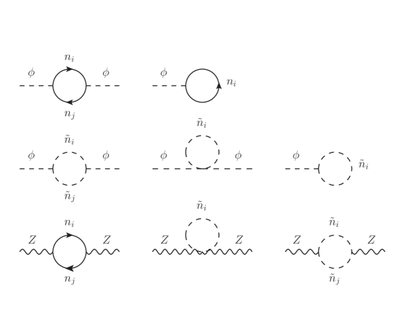
Figure 1: Generic one-loop Feynman-diagrams contributing to the computation of the one-loop new corrections to the Higgs boson mass form neutrinos and sneutrinos. Here $\phi=h,H,A$.

Following a similar analysis here as the one performed in [16] for the one generation case, it is illustrative to expand the renormalized self-energy in powers of $m_{D}$:

$$\hat{\Sigma}^{\nu/\tilde{\nu}}(p^{2})=\Big{(}\hat{\Sigma}^{\nu/\tilde{\nu}}(p^{2})\Big{)}_{m_{D}^{0}}+\Big{(}\hat{\Sigma}^{\nu/\tilde{\nu}}(p^{2})\Big{)}_{m_{D}^{2}}+\Big{(}\hat{\Sigma}^{\nu/\tilde{\nu}}(p^{2})\Big{)}_{m_{D}^{4}}+\dots$$ (117)

where $\Big{(}\hat{\Sigma}^{\nu/\tilde{\nu}}(p^{2})\Big{)}_{m_{D}^{n}}$ means $\mathcal{O}(m_{D}^{n})$ terms in the expansion of $\hat{\Sigma}^{\nu/\tilde{\nu}}(p^{2})$ in powers of $m_{D}$. For the present case with three generations $m_{D}^{2}$ represents shortly products of two Dirac matrices, such as, $m_{D}^{\dagger}m_{D}$ or $m_{D}m_{D}^{T}$; equivalently, $m_{D}^{4}$ refers to combinations of four matrices.

The first term in this expansion is independent of both $m_{D}$ and $m_{M}$, and represents, therefore, the pure gauge contribution (i.e. the result for $Y_{\nu}=0$), which is already present in the MSSM. On the other hand, the term proportional to $m_{D}^{4}$ is actually of order $\mathcal{O}(m_{D}^{4}/m_{M}^{2})$ (see [16] for details), so it is suppressed by the Majorana mass; higher order terms in this expansion are also suppressed by inverse powers of the Majorana mass. Thus, the new relevant contributions, coming from the neutrino and sneutrino sectors are those governed by the Yukawa couplings, and can arise only from the order $\mathcal{O}(m_{D}^{2})$ terms. Thus we have:

$$\Big{(}\hat{\Sigma}^{\nu/\tilde{\nu}}(p^{2})\Big{)}_{\rm{full}} =\Big{(}\hat{\Sigma}^{\nu/\tilde{\nu}}(p^{2})\Big{)}_{\rm{gauge}}+\Big{(}\hat{\Sigma}^{\nu/\tilde{\nu}}(p^{2})\Big{)}_{\rm{Yukawa}}\ ,$$ (118a)

$$\Big{(}\hat{\Sigma}^{\nu/\tilde{\nu}}(p^{2})\Big{)}_{\rm{gauge}} =\Big{(}\hat{\Sigma}^{\nu/\tilde{\nu}}(p^{2})\Big{)}_{m_{D}^{0}}\ ,$$ (118b)

$$\Big{(}\hat{\Sigma}^{\nu/\tilde{\nu}}(p^{2})\Big{)}_{\rm{Yukawa}} =\Big{(}\hat{\Sigma}^{\nu/\tilde{\nu}}(p^{2})\Big{)}_{m_{D}^{2}}+\mathcal{O}\Big{(}\frac{m_{D}^{4}}{m_{M}^{2}}\Big{)}\ .$$ (118c)

In the one generation case, the Dirac mass is related to the light, $m_{\nu}$, and heavy, $m_{N}$, neutrino physical masses by [16] $m_{D}^{2}=-m_{\nu}m_{N}\approx-m_{\nu}m_{M}$. In the three generations case, a similar functional dependence of $m_{D}^{2}$ with the physical masses in $m_{\nu}^{\rm diag}$ and in $m_{N}^{\rm diag}$ is found, as it is explicitely manifested in the parametrization of (20). This means that the Yukawa contribution in (118c), being proportional to $m_{D}^{2}$, grows with the Majorana masses, therefore leading to potential non-decoupling effects with respect to these masses. The question now is whether such a term is present in the renormalized self-energy and, in that case, if it is numerically relevant. This issue was first analyzed for the one generation case in [16], and recently in [17], showing that the presence and relevance of the $\mathcal{O}(m_{D}^{2})$ term in (118c) depends on the chosen renormalization scheme for $\tan\beta$.

In order to better understand where these differences come from, it is interesting to look first for the $\mathcal{O}(m_{D}^{2})$ terms in the bare self-energy, where the choice of the renormalization scheme does not enter. We will focus here on the lightest ${\cal CP}$-even Higgs boson self-energy, but the conclusions will be the same for the full $(h,H)$ system. By computing the one-loop contributions from the $hh$ diagrams in Fig. 1 we have obtained the following analytical result for the $\mathcal{O}(m_{D}^{2})$ contributions from three generations of neutrinos and sneutrinos to the bare self-energy:

$$\Big{(}\Sigma^{\nu/\tilde{\nu}}_{hh}(p^{2})\Big{)}_{m_{D}^{2}} = \displaystyle{\frac{g^{2}}{64\pi^{2}M_{W}^{2}\sin^{2}\beta}\sum_{i=1}^{3}\Big{(}m_{D}^{\dagger}m_{D}\Big{)}_{ii}\Bigg{\{}\Big{[}\Delta+1-\log\frac{m_{M_{i}}^{\ 2}}{\mu_{\overline{\text{DR}}}^{2}}\Big{]}}$$ (119)

$$\times \Big{(}\big{(}p^{2}-M_{Z}^{2}\big{)}2\cos^{2}\alpha$$

$$-M_{Z}^{2}\sin^{2}\beta\big{(}\cos^{2}\alpha(4-3\cot^{2}\beta)+2\sin 2\alpha\cot\beta-\sin^{2}\alpha\big{)}\Big{)}$$

$$+ \displaystyle{\Big{[}\Delta-\log\frac{m_{M_{i}}^{2}}{\mu_{\overline{\text{DR}}}^{2}}\Big{]}(4m^{2}_{\text{SUSY}}\cos^{2}\alpha)}\Bigg{\}}\ .$$

In this expression, for shortness, we have set $a_{\nu}=b_{\nu}=\mu=0$, and we have considered the most simple case with just one single soft mass scale in the slepton sector, $m_{\tilde{L}_{i}}=m_{\tilde{R}_{j}}=:m_{\text{SUSY}}$, with $i=1,2,3$. $\Delta$ is defined in (107) and $\mu_{\overline{\text{DR}}}$ is again the renormalization scale. The corresponding result for the $\Sigma_{HH}$ is obtained from the above formula by replacing $\cos\alpha\rightarrow\sin\alpha,\,\sin\alpha\rightarrow-\cos\alpha$.

First of all, it should be noted that the result in (119) is a pure ${\cal O}(Y_{\nu}^{2})$ radiative correction with an overall factor given by:

$${\frac{g^{2}}{64\pi^{2}M_{W}^{2}\sin^{2}\beta}\sum_{i=1}^{3}\Big{(}m_{D}^{\dagger}m_{D}\Big{)}_{ii}=\frac{1}{32\pi^{2}}\sum_{i=1}^{3}\Big{(}Y_{\nu}^{\dagger}Y_{\nu}\Big{)}_{ii}.}$$ (120)

Secondly, a good check of our computation in (119) is that by setting to zero all the entries in the $m_{D_{ij}}$ matrix except for one in the diagonal (for instance, $m_{D_{11}}$) we recover the result of the one generation case, in full agreement with the expressions in the Appendix A of [17] (with $m_{D_{11}}=m_{D}$ and $m_{M_{1}}=m_{M}$).

The result in (119) shows, most importantly, that the bare self-energy has a non-negligible $\mathcal{O}(m_{D}^{2})$ term, which grows logarithmically with the Majorana masses. Nevertheless, as we have already said, we will analyze whether such a term is present or not in the renormalized self-energy. If one assumes that the Yukawa contribution from neutrinos/sneutrinos to the bare self-energy is approximated by the previous result in (119), one arrives at the following $\mathcal{O}(m_{D}^{2})$ expressions for the $\tan\beta$ counterterms in the various schemes:

$$(\delta\tan\beta^{\overline{\text{DR}}})_{m_{D}^{2}} = \displaystyle{-\frac{g^{2}}{64\pi^{2}M_{W}^{2}\sin^{2}\beta}\sum_{i=1}^{3}\Big{(}m_{D}^{\dagger}m_{D}\Big{)}_{ii}\Big{[}\Delta\Big{]}},$$

$$(\delta\tan\beta^{\text{m}\overline{\text{DR}}})_{m_{D}^{2}} = \displaystyle{-\frac{g^{2}}{64\pi^{2}M_{W}^{2}\sin^{2}\beta}\sum_{i=1}^{3}\Big{(}m_{D}^{\dagger}m_{D}\Big{)}_{ii}\Big{[}\Delta-\log\frac{m_{M_{i}}^{\ 2}}{\mu_{\overline{\text{DR}}}^{2}}\Big{]}},$$

$$(\delta\tan\beta^{\rm OS})_{m_{D}^{2}} = (\delta\tan\beta^{\rm DEC})_{m_{D}^{2}}=(\delta\tan\beta^{\rm HM})_{m_{D}^{2}}=$$ (121)

$$\displaystyle{-\frac{g^{2}}{64\pi^{2}M_{W}^{2}\sin^{2}\beta}\sum_{i=1}^{3}\Big{(}m_{D}^{\dagger}m_{D}\Big{)}_{ii}\Big{[}\Delta+1-\log\frac{m_{M_{i}}^{\ 2}}{\mu_{\overline{\text{DR}}}^{2}}\Big{]}}.$$

Then, one can easily find the relation among the corresponding renormalized $\tan\beta$ values, at this same level of approximation. Using, for instance, the renormalized value in the OS scheme, $\tan\beta^{\rm OS}$, which is $\mu_{\overline{\text{DR}}}$ independent, as the reference value to be compared with in this illustrative exercise, we get:

$$(\tan\beta^{\rm OS})_{m_{D}^{2}} = (\tan\beta^{\rm DEC})_{m_{D}^{2}}=(\tan\beta^{\rm HM})_{m_{D}^{2}},$$

$$(\tan\beta^{\overline{\text{DR}}})_{m_{D}^{2}}-(\tan\beta^{\rm OS})_{m_{D}^{2}} = \displaystyle{-\frac{g^{2}\tan\beta}{64\pi^{2}M_{W}^{2}\sin^{2}\beta}\sum_{i=1}^{3}\Big{(}m_{D}^{\dagger}m_{D}\Big{)}_{ii}\Big{[}1-\log\frac{m_{M_{i}}^{\ 2}}{\mu_{\overline{\text{DR}}}^{2}}\Big{]}},$$

$$(\tan\beta^{\text{m}\overline{\text{DR}}})_{m_{D}^{2}}-(\tan\beta^{\rm OS})_{m_{D}^{2}} = \displaystyle{-\frac{g^{2}\tan\beta}{64\pi^{2}M_{W}^{2}\sin^{2}\beta}\sum_{i=1}^{3}\Big{(}m_{D}^{\dagger}m_{D}\Big{)}_{ii}\Big{[}1\Big{]}}.$$ (122)

Finally, using the computed expressions at $\mathcal{O}(m_{D}^{2})$ of the bare self-energy and the counterterms one obtains the renormalized self-energy at this same order. In the case of the $\overline{\text{DR}}$ scheme we get:

$$\Big{(}\hat{\Sigma}^{\nu/\tilde{\nu}\,\,{\overline{\text{DR}}}}_{hh}(p^{2})\Big{)}_{m_{D}^{2}} = \displaystyle{\frac{g^{2}}{64\pi^{2}M_{W}^{2}\sin^{2}\beta}\sum_{i=1}^{3}\Big{(}m_{D}^{\dagger}m_{D}\Big{)}_{ii}\Big{[}1-\log\frac{m_{M_{i}}^{\ 2}}{\mu_{\overline{\text{DR}}}^{2}}\Big{]}}$$ (123)

$$\times \Big{[}-2M_{A}^{2}\cos^{2}(\alpha-\beta)\cos^{2}\beta+2p^{2}\cos^{2}\alpha$$

$$-M_{Z}^{2}\sin\beta\sin(\alpha+\beta)\left(2\left(1+\cos^{2}\beta\right)\cos\alpha-\sin 2\beta\sin\alpha\right)\Big{]},$$

which can be rewritten in terms of $m_{h,{\rm tree}}$ simply as:

$$\Big{(}\hat{\Sigma}^{\nu/\tilde{\nu}\,\,{\overline{\text{DR}}}}_{hh}(p^{2})\Big{)}_{m_{D}^{2}} = \displaystyle{\frac{g^{2}}{64\pi^{2}M_{W}^{2}\sin^{2}\beta}\sum_{i=1}^{3}\Big{(}m_{D}^{\dagger}m_{D}\Big{)}_{ii}\Big{[}1-\log\frac{m_{M_{i}}^{\ 2}}{\mu_{\overline{\text{DR}}}^{2}}\Big{]}}$$ (124)

$$\times \Big{[}\big{(}p^{2}-m_{h,\text{tree}}^{2}\big{)}2\cos^{2}\alpha-M_{Z}^{2}\sin 2\beta\sin 2(\alpha+\beta)\Big{]}.$$

Notice that there are no terms proportional to $m_{\rm SUSY}^{2}$ in (124), since they are cancelled by the $\delta T_{h},\delta T_{H},\delta M_{A}^{2}$ and $\delta M_{Z}^{2}$ counterterms. We have numerically studied the accuracy of these approximate $\mathcal{O}(m_{D}^{2})$ results, both for the renormalized self-energy and the finite contribution in the bare self-energy, and compared with their corresponding full results. We have found that they constitute extremely good approximations, leading to relative differences below $10^{-4}$ w.r.t. the full expressions for all the explored parameter space (including for non-zero values of $a_{\nu}$, $b_{\nu}$ and $\mu$).

It is also straight forward to check that by setting properly the $m_{D}$ matrix entries in (123) and (124) we recover again the proper results for the one generation case, in agreement with [16] and [17].

Similarly, one can derive the corresponding $\mathcal{O}(m_{D}^{2})$ expressions in the other considered schemes. In the $\text{m}\overline{\text{DR}}$ we get:

$$\Big{(}\hat{\Sigma}^{\nu/\tilde{\nu}\,\,{\text{m}\overline{\text{DR}}}}_{hh}(p^{2})\Big{)}_{m_{D}^{2}} = \displaystyle{\frac{g^{2}}{64\pi^{2}M_{W}^{2}\sin^{2}\beta}\sum_{i=1}^{3}\Big{(}m_{D}^{\dagger}m_{D}\Big{)}_{ii}\Big{[}1\Big{]}}$$ (125)

$$\times \Big{[}\big{(}p^{2}-m_{h,\text{tree}}^{2}\big{)}2\cos^{2}\alpha-M_{Z}^{2}\sin 2\beta\sin 2(\alpha+\beta)\Big{]}.$$

And in the OS, DEC and HM we get the expected decoupling behavior at this order, in agreement with the results for the one generation case in [16] and [17]:

$$\Big{(}\hat{\Sigma}^{\nu/\tilde{\nu}\,\,{\rm OS}}_{hh}(p^{2})\Big{)}_{m_{D}^{2}} = \Big{(}\hat{\Sigma}^{\nu/\tilde{\nu}\,\,{\rm DEC}}_{hh}(p^{2})\Big{)}_{m_{D}^{2}}=\Big{(}\hat{\Sigma}^{\nu/\tilde{\nu}\,\,{\rm HM}}_{hh}(p^{2})\Big{)}_{m_{D}^{2}}$$ (126)

$$= \displaystyle{\frac{g^{2}}{64\pi^{2}M_{W}^{2}\sin^{2}\beta}\sum_{i=1}^{3}\Big{(}m_{D}^{\dagger}m_{D}\Big{)}_{ii}\Big{[}0\Big{]}}$$

$$\times \Big{[}\big{(}p^{2}-m_{h,\text{tree}}^{2}\big{)}2\cos^{2}\alpha-M_{Z}^{2}\sin 2\beta\sin 2(\alpha+\beta)\Big{]}.$$

In summary, in this section we have analyzed the relevant differences among the various schemes for $\tan\beta$ and the wave function renormalizations, and these differences have been understood in terms of $\mathcal{O}(m_{D}^{2})$ contributions to the self-energies. Once we have set clearly these differences, it is a simple exercise to find the prediction in one scheme and then extract from it the prediction in another scheme.

We illustrate numerically the most relevant differences among the various schemes in Fig. 2. The plot on the left displays the renormalized self-energies in three schemes that are $\mu_{\overline{\text{DR}}}$ independent: OS, DEC and $\text{m}\overline{\text{DR}}$. In all the cases we plot the full one-loop result from neutrinos and sneutrinos evaluated at the tree Higgs mass, $p^{2}=m_{h,{\rm tree}}^{2}$, as a function of $M_{A}$. In this example the instabilities that are found in the OS scheme are clearly visible, in comparison with the stability of the $\text{m}\overline{\text{DR}}$ and DEC schemes. These “dips” are due to thresholds encountered in the loop diagrams and, as can be seen in Fig. 2, appear at $M_{A}$ values approximately twice each one of the soft SUSY-breaking parameters $m_{\tilde{L}_{i}}$. We have checked that these “dips” are indeed very narrow and profound. For aritrary close values to threshold they go to $-\infty$ due to the fact that the imaginary part of the standard one-loop $B_{0}$ function[76] is not differentiable at threshold. These instabilities occur as long as width effects are not taken into account. We also see that, for the input values in this plot, the numerical values for the renormalized self-energies of the OS, DEC and $\text{m}\overline{\text{DR}}$ are quite close to each other. In particular, in the region out of the dips, the OS and DEC values are practically identical. We have also checked that the numerical results in the HM scheme (not shown) also manifest instabilities and, furthermore, they turn out to be substantially different than in the other $\mu_{\overline{\text{DR}}}$ independent schemes. This difference of the HM has been studied in [17] in the one generation case and it has been understood in terms of the substantially different contributions in the pure gauge part, i.e of $\mathcal{O}(m_{D}^{0})$, which are numerically relevant. For instance, comparing the HM with the DEC approximate results for the mass correction in [17], the first one is a factor of $(\cos^{2}2\beta)^{-1}$ larger than the last one (for $\tan\beta=2$, e.g., this yields a factor of 2.8). We have found agreement with this numerical factor in our numerical results for $\hat{\Sigma}^{\nu/\tilde{\nu}\,\,{\rm HM}}_{hh}(m_{h,\text{tree}}^{2})$, in the region out of the instabilities.

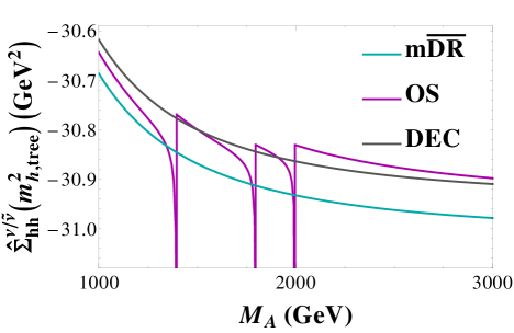
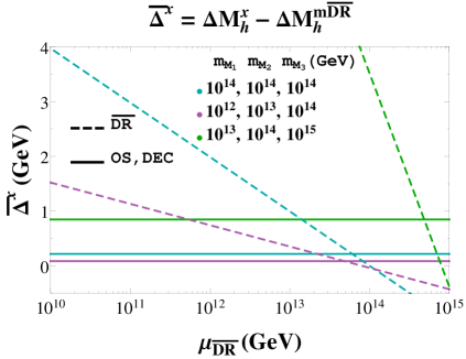
Figure 2: Comparison among the various schemes. The plot in the left shows the renormalized self-energies evaluated at $p^{2}=m_{h,{\rm tree}}^{2}$ in the OS, DEC and $\text{m}\overline{\text{DR}}$ as functions of $M_{A}$, for $m_{M_{1,2,3}}=10^{12}~{}{\rm GeV}$, $m_{\nu_{1}}=0.01~{}{\rm eV}$ and $m_{\tilde{L}_{1,2,3}}=(700,900,1000)~{}{\rm GeV}$. The plot in the right shows the predictions of the mass differences ${\overline{\Delta}}^{\rm x}=\Delta M_{h}^{\rm x}-\Delta M_{h}^{\text{m}\overline{\text{DR}}}$, for ${\rm x}={\overline{\text{DR}}}$ (dashed lines), OS, DEC (solid lines) , as functions of $\mu_{\overline{\text{DR}}}$, and for several choices of the Majorana masses, $(m_{M_{1}},m_{M_{2}},m_{M_{3}})$(GeV): $(10^{14},10^{14},10^{14})$ (in light blue); $(10^{12},10^{13},10^{14})$ (in purple) and $(10^{13},10^{14},10^{15})$ (in green). The rest of input parameters are fixed as in (127). $\Delta M_{h}$ is defined in (92).

The right plot of Fig. 2 compares the predictions for the Higgs mass correction among the different renormalization schemes in various examples with different choices for the Majorana masses and their hierarchies. Again the full one-loop renormalized self-energies are considered and the simple formula for the Higgs mass correction in (92) is used. In this plot we have chosen the $\text{m}\overline{\text{DR}}$ as the reference scheme to be compared with, such that ${\overline{\Delta}}^{\rm x}=\Delta M_{h}^{\rm x}-\Delta M_{h}^{\text{m}\overline{\text{DR}}}$ represents the difference in the prediction of the mass correction in the scheme $x$ respect to the prediction in the $\text{m}\overline{\text{DR}}$ scheme. Firstly, we have found again that the results of the OS and the DEC schemes are practically indistinguishable. We also see that for the input values explored in this plot, the predictions in these OS and DEC schemes differ from the predictions in the $\text{m}\overline{\text{DR}}$ scheme in $1\,\,\mathrm{GeV}$ at most, and this largest difference is for the case when the heaviest Majorana mass is at the largest considered value of $10^{15}\,\,\mathrm{GeV}$. The comparison with the $\overline{\text{DR}}$ scheme, whose result is $\mu_{\overline{\text{DR}}}$ dependent, shows that, in order to get a prediction close to the other schemes, within say a 1 GeV interval, a value of $\mu_{\overline{\text{DR}}}$ at the near proximity of the highest Majorana mass should be chosen.

5 Numerical analysis of $\mathbf{\Delta M_{h}}$

In this final section we show some numerical results for the one-loop corrections to the light Higgs boson mass, $\Delta M_{h}$ (via (92)). Using the DEC scheme, the OS scheme or another scheme that decouples the heavy mass scales completely, would yield small effects (except where the numerical instabilities occur as demonstrated in Sect. 3.3). Since every scheme, however, has its advantages and disadvantages as discussed in Sect. 3.3 we choose here to use the $\text{m}\overline{\text{DR}}$ scheme. The numerical results in other schemes can be inferred from these by using the results in the previous section. While by definition not showing full decoupling, the $\text{m}\overline{\text{DR}}$ combines several of the desired properties: stability, perturbativity and gauge invariance at the one-loop level. Besides, this scheme is safe of large logarithms introduced by the large Majorana scales. The fact that the non-logarithmic finite terms are not removed in this scheme, translates into a finite contribution of $\mathcal{O}(m_{D}^{2})$ which will leave a non-vanishing radiative contribution from the neutrinos and sneutrinos into the Higgs mass correction. Furthermore, we are interested in different scenarios where the Majorana masses can range from the extreme large values of order $10^{14}-10^{15}$ GeV down to low values of order $10^{3}$ GeV and, correspondingly, we will explore these scenarios keeping explicitly the contributions from the $\nu/\tilde{\nu}$ particles. Consequently, the numerical analysis is performed as a function of all relevant parameters that will be varied in a wide range: the masses of the light neutrinos, the masses of the heavy Majorana neutrinos and the mixing provided by the $R$ matrix in the case of three generations, as well as the MSSM parameters. Unless stated otherwise, we set the parameters to the following reference values:

$$\begin{array}[]{rcl}m_{M_{1}}=m_{M_{2}}=m_{M_{3}}\equiv m_{M}=10^{14}\text{ GeV}\,,&&m_{\nu_{1}}=0.1\text{ eV}\,,\\ m_{\tilde{L}_{1}}=m_{\tilde{L}_{2}}=m_{\tilde{L}_{3}}\equiv m_{\tilde{L}}=2\text{ TeV}\,,&&M_{A}=500\text{ GeV}\,,\\ m_{\tilde{R}_{1}}=m_{\tilde{R}_{2}}=m_{\tilde{R}_{3}}\equiv m_{\tilde{R}}=2\text{ TeV}\,,&&\mu=500\text{ GeV}\,,\\ a_{\nu}=2\text{ TeV}\,,&&\tan\beta=2\,,\\ b_{\nu}=2\text{ TeV}\,,&&R={\rm 1\kern-1.19995pt\rule{0.3pt}{6.45831pt}\raisebox{0.0pt}{\rule{1.00006pt}{0.3pt}}}.\end{array}$$ (127)

The masses of the other two light neutrinos are obtained from $m_{\nu_{1}}$ and the mass differences given in (2.1), implying that these light neutrinos of our reference case are quasi-degenerate.

We assume that the other MSSM parameters, in particular from the top/scalar top sector, which do not affect our results, give a corrected Higgs mass of $M_{h}\sim 125\,\,\mathrm{GeV}$. Here it should be noted that in the non-(s)neutrino part of the calculation a $\overline{\mathrm{DR}}$ renormalization of $\tan\beta$ and the wave function of the two Higgs doublets has been used (with $\mu_{\overline{\text{DR}}}=m_{t}$). The choice of a different renormalization scale in the estimate of $M_{h}$ within the MSSM has been discussed at length in the literature (see for instance Refs. [66, 67]), but it is not relevant for the present work given the fact that we are using this $M_{h}$ as a given value (fixed here to $125\,\,\mathrm{GeV}$) and we are estimating just the shift $\Delta M_{h}$ with respect to this value due to the new sectors $\nu/\tilde{\nu}$ (given by (92)).

Two different scenarios for the mass hierarchy of the light neutrinos can be set, the normal hierarchy (NH) case and the inverted hierarchy (IH) case:

• Normal hierarchy (NH):
  $\nu_{1}$ is the lightest neutrino, and its mass will be our input value. The mass of the other two neutrinos are fixed by the experimental mass differences:

  $$m_{\nu_{2}}^{{\rm NH}} = \sqrt{m_{\nu_{1}}^{2}+\Delta m_{21}^{2}}\,,$$

  $$m_{\nu_{3}}^{{\rm NH}} = \sqrt{m_{\nu_{1}}^{2}+\Delta m_{21}^{2}+\Delta m_{32}^{2}}\,.$$ (128)

• Inverted hierarchy (IH):
  $\nu_{3}$ is the lightest neutrino, and its mass will be our input value. The mass of the other two neutrinos again, are fixed by the experimental mass differences:

  $$m_{\nu_{1}}^{{\rm IH}} = \sqrt{m_{\nu_{3}}^{2}-\Delta m_{21}^{2}-\Delta m_{32}^{2}}\,,$$

  $$m_{\nu_{2}}^{{\rm IH}} = \sqrt{m_{\nu_{3}}^{2}-\Delta m_{32}^{2}}\,.$$ (129)

with $\Delta m_{21}^{2}$ and $\Delta m_{32}^{2}$ are given in section 2. The default choice used below is the NH case, and the IH case will be especially indicated.

Notice that we are using the Casas-Ibarra parametrization (20) that provides a prediction of the full $3\times 3$ $v_{2}Y_{\nu}$ (i.e. $m_{D}$) matrix in terms of the input parameters of the light sector, $m_{\nu_{i}}$ and $\theta_{ij}$, and of the heavy sector $m_{M_{i}}$ and $\theta_{i}$, and the last two can take in principle any value. Therefore the size of the Yukawa couplings that we are generating is related directly to these parameters, and in consequence they can be large and even non-perturbative. In order to ensure that $Y_{\nu}$ is inside the perturbative region, for every set of input parameters we first check that all of the entries of the Yukawa matrix fulfill a perturbative condition that we set here to

$$\dfrac{|(Y_{\nu})_{ij}|^{2}}{4\pi}<1.5,$$ (130)

otherwise, the point in the parameter space is rejected.

5.1 Relation with the one-generation case

As a first check of our three generations code, we have reproduced with this code the same behavior of the Higgs mass correction, $\Delta M_{h}$, with the Majorana mass as in the one generation case [16]. The connection with the one generation case is done by setting the corresponding absent entries in the Dirac mass matrix to zero. For this analysis, the mass of the light and heavy Majorana neutrinos have been set to $0.1$ eV and $10^{14}\,\,\mathrm{GeV}$ respectively. The result for the one-generation case delivered in such a way is shown in the left plot of Fig. 3. In the right plot it is shown the behavior of the three generations case with three equaly heavy neutrino masses, i.e. $m_{M_{i}}=m_{M}$. As expected, we obtain that the Higgs mass corrections in the three generations case are three times the ones of the one generation case. Notice that we have separated the contributions to the full mass correction coming from the gauge and the Yukawa parts, according to (118a):

$$\Delta M_{h}=\left(\Delta M_{h}\right)_{\text{gauge}}+\left(\Delta M_{h}\right)_{\text{Yukawa}}\,,$$ (131)

where $\left(\Delta M_{h}\right)_{\text{gauge}}$ corresponds to setting all the Yukawa couplings to zero and $\left(\Delta M_{h}\right)_{\text{Yukawa}}$ is the remaining contribution. Within our approximation of (92), they are related with the renormalized self energy as follows:

$$\left(\Delta M_{h}\right)_{\text{gauge}} =-\dfrac{\hat{\Sigma}^{\nu/\tilde{\nu}}_{\text{gauge}}(M_{h}^{2})}{2M_{h}},$$ (132a)

$$\left(\Delta M_{h}\right)_{\text{Yukawa}} =-\dfrac{\hat{\Sigma}^{\nu/\tilde{\nu}}_{\text{Yukawa}}(M_{h}^{2})}{2M_{h}}\equiv\hat{\Delta}M_{h}\,.$$ (132b)

It should also be noted that, similarly to the one generation case, the full mass correction changes from positive values in the low $m_{M}$ region to negative values in the region of large $m_{M}\;\raisebox{-3.00003pt}{$\stackrel{{\scriptstyle\displaystyle>}}{{\sim}}$}\;10^{14}\,\,\mathrm{GeV}$. In particular, for the reference values in (127), it is $\Delta M_{h}=-0.25\,\,\mathrm{GeV}$.

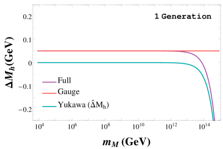
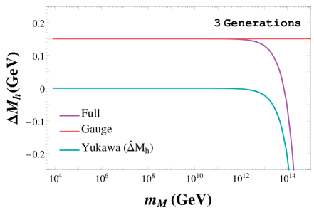
Figure 3: Left panel: $\Delta M_{h}$ as a function of $m_{M}$ for the one generation case. Right panel: $\Delta M_{h}$ as a function of the scale $m_{M}$ for the degenerate three generations case. The rest of the model parameters are set as in (127).

As mentioned before, the gauge part of the Higgs mass correction represents the common part with the MSSM, therefore in the following, we will focus the discussion mainly in the Yukawa part which is the new contribution, denoted here and from now on shortly as $\hat{\Delta}M_{h}$.

5.2 Sensitivity of the Higgs mass correction to the relevant SUSY parameters

We next study the effects on $\Delta M_{h}$ of the other parameters entering the calculation: $\tan\beta$, $M_{A}$, $m_{\tilde{L}_{i}}$, $m_{\tilde{R}_{i}}$, $a_{\nu}$, $b_{\nu}$ and $\mu$. In order to explore these behaviours of $\Delta M_{h}$ with the relevant MSSM parameters in presence of three Majorana neutrinos and their SUSY partners, we run with one of the parameters while the others are set to the reference values given in (127).

The behaviour of the one-loop corrections to the lightest Higgs boson mass in the $\text{m}\overline{\text{DR}}$ scheme with these relevant parameters are shown in figs 4 and 5.

We start with the analysis of the behaviour with $\tan\beta$, which is shown in Fig. 4. In the left plot the behavior of the full mass correction as well as the gauge and Yukawa parts are shown. In the right plot we focus on the Yukawa contribution to the mass correction. The biggest negative correction $\hat{\Delta}M_{h}$ is obtained for the lowest considered value of $\tan\beta=2$; so in the following, motivating $\tan\beta=2$ as our reference value. The numerical results for other choices of $\tan\beta$ in the remaining plots of this work can be easily inferred from this plot on the right.

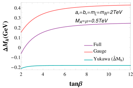
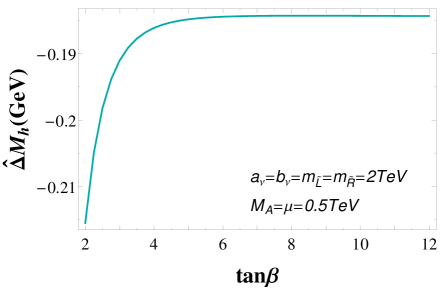
Figure 4: Left panel: The full, gauge and Yukawa contributions to $\Delta M_{h}$ defined in (131), (132a) and (132b), respectively, are plotted as functions of $\tan\beta$. Right panel: Zoom of $\hat{\Delta}M_{h}$ as a function of $\tan\beta$.

The dependence on the pseudoscalar Higgs boson mass is analyzed in Fig. 5. For $M_{A}$ larger than 200 GeV the behavior with $M_{A}$ is nearly flat. The dependence on the soft SUSY-breaking mass of the “left handed” $SU(2)$ doublet, $m_{\tilde{L}}$ is also flat as shown in Fig. 5. The behavior with the soft mass of the “right handed” sector $m_{\tilde{R}}$ in a range similar to the other soft SUSY-breaking parameters is shown in Fig. 5. In addition, also values of $m_{\tilde{R}}$ closer to $m_{M_{i}}$ are explored in this figure. The correction to the Higgs boson $h$ mass stays flat with $m_{\tilde{R}}$ up to about $m_{\tilde{R}}\sim 10^{13}\,\,\mathrm{GeV}$. Above this mass scale the correction grows rapidly, reaching $\Delta M_{h}\sim-1$ GeV at $m_{\tilde{R}}\sim 10^{14}\,\,\mathrm{GeV}$, in agreement with the results found for the one generation case in [16].

We have also checked that the behavior of $\Delta M_{h}$ with the remaining parameters, $a_{\nu}$, $b_{\nu}$ and $\mu$, in the intervals $-1000\text{ GeV}<a_{\nu}<1000\text{ GeV}$, $100\text{ GeV}<b_{\nu}<10^{4}\text{ GeV}$ and $-1000\text{ GeV}<\mu<1000\text{ GeV}$ are also flat as in the case of the low mass values of $m_{\tilde{R}}$. The behaviors of $\hat{\Delta}M_{h}$ with all these parameters agree as well with the results obtained in the one-generation case [16].

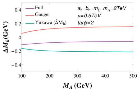
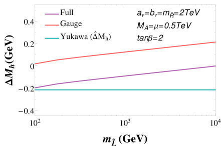
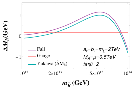
Figure 5: Left upper panel: $\Delta M_{h}$ as a function of $M_{A}$. Upper right panel: $\Delta M_{h}$ as a function of $m_{\tilde{L}}$. Lower left panel: $\Delta M_{h}$ as a function of $m_{\tilde{R}}$ for low mass values $10^{2}\text{ GeV}<m_{\tilde{R}}<10^{4}\text{ GeV}$. Lower right panel: $\Delta M_{h}$ as a function of $m_{\tilde{R}}$ for high mass values $10^{13}\text{ GeV}<m_{\tilde{R}}<10^{14}\text{ GeV}$.

5.3 Sensitivity of the Higgs mass corrections to the light neutrinos

In this section we analyze the sensitivity of the mass correction to the mass hierarchy of the light neutrinos. Here we investigate the two cases of NH and IH, where the values of the rest of the parameters are fixed to the ones of our reference scenario given in (127).

Fig. 6 shows the behavior of the Yukawa part of the mass correction with the mass of the lightest neutrino, $\nu_{1}$ and $\nu_{3}$ for the NH (solid lines) and IH (dashed lines), respectively. We show the Yukawa contribution to the mass correction (vertical left axis) as well as the sum of the three neutrino masses (vertical right axis) for each value as a function of the lightest neutrino mass.

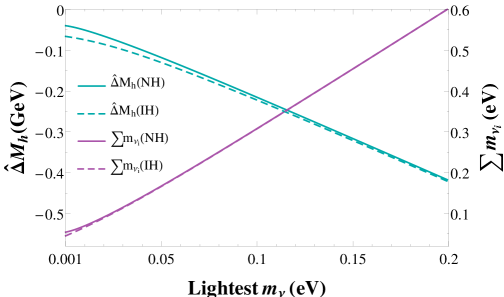
Figure 6: $\hat{\Delta}M_{h}$ (blue) and $\Sigma\,m_{\nu_{i}}$ (purple) as a function of the lightest neutrino mass, $m_{\nu_{1}}$ for a normal hierarchy (solid) and $m_{\nu_{3}}$ for an inverted hierarchy (dashed). The rest of the model parameters are set as in (127).

We conclude that, even though the numerical result of $\hat{\Delta}M_{h}$ for both hierarchies are quite similar, the Higgs mass corrections found in the IH case are slightly bigger than the ones of the NH case.

5.4 Sensitivity of the Higgs mass corrections to the heavy neutrino masses

In this section the behaviors of the mass correction with the masses of the heavy Majorana neutrinos as well as with the $R$ matrix are analyzed. As mentioned before, the $R$ matrix of (20) parametrizes the mixing in the heavy neutrino sector.

First of all, we show the results for the degenerate heavy neutrino scenario where the three heavy Majorana neutrinos have all the same mass, i.e. $m_{M_{1}}=m_{M_{2}}=m_{M_{3}}=m_{M}$. The mass of the lightest neutrino as well as the SUSY parameters are set to the reference values given in (127). In the left panel of Fig. 7 we show the behaviour of the full mass correction $\Delta M_{h}$ with the common Majorana $m_{M}$. We have separated the contribution to the mass correction coming from the neutrino and sneutrino sectors in order to show the remarkable cancellation between the two parts that it is happening. It can also be seen that the behavior of the total $\Delta M_{h}$ with $m_{M}$ at very large $m_{M}\gtrsim 10^{14}\,\,\mathrm{GeV}$ is dominated by the neutrino contributions.

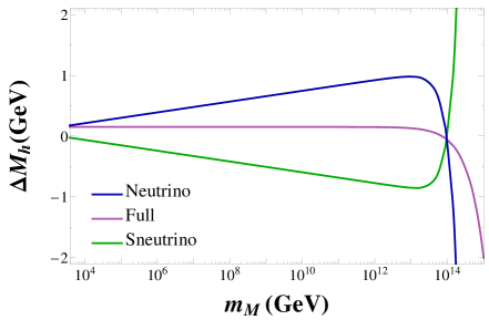
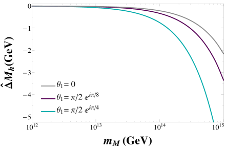
Figure 7: Left panel: $\Delta M_{h}$ as a function of $m_{M}$ for degenerate heavy neutrinos and $R=1$. The corrections from neutrinos, sneutrinos and the total are displayed separately. Right panel: $\hat{\Delta}M_{h}$ as a function of $m_{M}$ for $\theta_{1}=\left(0,\pi/2e^{i\pi/8},\pi/2e^{i\pi/4}\right)$ and $\theta_{2}=\theta_{3}=0$. The rest of the model parameters are set as in (127).

It should be noted that the same result as in Fig. 7 is obtained for any other real $R$ matrix different from the reference value $R={\rm 1\kern-1.19995pt\rule{0.3pt}{6.45831pt}\raisebox{0.0pt}{\rule{1.00006pt}{0.3pt}}}$. This independence on the particular real $R$ value can be understood from the fact that, as we have mentioned before, $\hat{\Delta}M_{h}\varpropto m_{D}^{\dagger}m_{D}$, and with the definition of $m_{D}$ given in (20), we find:

$$m_{D}^{\dagger}m_{D} = \sqrt{m_{N}^{\text{diag}}}\,R^{*}\,\sqrt{m_{\nu}^{\text{diag}}}\,U_{\text{PMNS}}^{T}\,U_{\text{PMNS}}^{*}\,\sqrt{m_{\nu}^{\text{diag}}}\,R^{T}\sqrt{m_{N}^{\text{diag}}}$$ (133)

$$= \sqrt{m_{N}^{\text{diag}}}\,R^{*}\,m_{\nu}^{\text{diag}}\,R^{T}\sqrt{m_{N}^{\text{diag}}}\,.$$

As the three light neutrinos in (127) are quasi degenerate, $m_{\nu}^{\text{diag}}\thickapprox m_{\nu_{1}}{\rm 1\kern-1.19995pt\rule{0.3pt}{6.45831pt}\raisebox{0.0pt}{\rule{1.00006pt}{0.3pt}}}$, and since here $R$ is a real and orthogonal matrix, then (133) becomes independent on $R$, i.e.:

$$m_{D}^{\dagger}m_{D}\thickapprox m_{\nu_{1}}\sqrt{m_{N}^{\text{diag}}}\,R\,R^{T}\sqrt{m_{N}^{\text{diag}}}=m_{\nu_{1}}m_{N}^{\text{diag}}\,.$$ (134)

In contrast, when a complex $R$ matrix is implemented, the result in (134) is no longer true and $\hat{\Delta}M_{h}$ grows with the size of both Re$(\theta_{i})$ and Im$(\theta_{i})$, as can be seen in the right panel of Fig. 7. There we plot $\hat{\Delta}M_{h}$ for three different values $\theta_{1}=\left(0,\pi/2e^{i\pi/8},\pi/2e^{i\pi/4}\right)$ while the other two angles, i.e. $\theta_{2}$ and $\theta_{3}$, are set to zero. We have checked that similar growing behaviors with the other complex $\theta_{2,3}$ angles are found.

Next we study the case where there is a hierarchy between the three heavy Majorana neutrino masses. First we consider the simplest case of $R={\rm 1\kern-1.19995pt\rule{0.3pt}{6.45831pt}\raisebox{0.0pt}{\rule{1.00006pt}{0.3pt}}}$ and analyze the behavior with the heaviest Majorana mass, chosen here to be $m_{M_{3}}$, while the other two masses are fixed to $m_{M_{1}}=10^{10}\,\,\mathrm{GeV}$ and $m_{M_{2}}=10^{11}\,\,\mathrm{GeV}$. Fig. 8 compares the behavior of $\hat{\Delta}M_{h}$ with $m_{M_{3}}$ in both degenerate and hierarchical cases. This figure shows that the size of the correction $\hat{\Delta}M_{h}$ in the hierarchical case is dominated by the heaviest Majorana mass, $m_{M_{3}}$ in this example. Furthermore, the obtained Higgs mass correction for a given $m_{M_{3}}$ value is smaller than the corresponding mass correction in the degenerate case with the common $m_{M}$ fixed to this same value, i.e for $m_{M}=m_{M_{3}}$ .

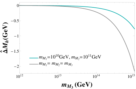
Figure 8: $\hat{\Delta}M_{h}$ as a function of $m_{M_{3}}$ for hierarchical (blue) and degenerate (grey) heavy neutrinos. The rest of input parameters are set to the reference values in (127).

In order to perform a complete analysis with hierarchical heavy neutrinos, we have scanned the Majorana masses $m_{M_{1}}$ and $m_{M_{2}}$ in the range $10^{12}\leqslant m_{M_{1,2}}\leqslant 10^{14}\,\,\mathrm{GeV}$ for two different values of $m_{M_{3}}$. As a result, we have obtained the two contour plots that are shown in Fig. 9. Due to the fact that we are assuming in practice that the light neutrinos are quasi degenerate and that there is no mixing among the heavy Majorana neutrinos ($R={\rm 1\kern-1.19995pt\rule{0.3pt}{6.45831pt}\raisebox{0.0pt}{\rule{1.00006pt}{0.3pt}}}$), the behavior of the Higgs mass correction is symmetric in all the three Majorana masses and consequently, the biggest correction is obtained when the three masses are equal and set to the highest value, i.e. $10^{14}\,\,\mathrm{GeV}$ in these plots. We have checked that once the value of $m_{M_{3}}$ lies below $10^{12}\,\,\mathrm{GeV}$ there is no appreciable sensitivity to that mass, so the result will be the same as in the left panel of Fig. 9. Similarly to the previous degenerate case, there is not sensitivity to the choice of the real $R$ matrix in the hierarchical case either, as can be understood from the result in (134) that also holds here. Therefore, the results in Fig. 9 are valid for all values of real $R$.

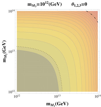
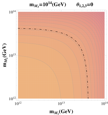
Figure 9: $\hat{\Delta}M_{h}$ as a function of $m_{M_{1}}$ and $m_{M_{2}}$ in the hierarchical heavy neutrinos scenario. Left panel: with $m_{M_{3}}=10^{12}\,\,\mathrm{GeV}$. Right panel: with $m_{M_{3}}=10^{14}\,\,\mathrm{GeV}$. The rest of input parameters are set to the reference values in (127).

Finally we analyze the imprints of the mixing of the hierarchical heavy neutrinos in $\hat{\Delta}M_{h}$ when a complex $R$ matrix is implemented. Fig. 10 shows the $\hat{\Delta}M_{h}$ contours in the general case of three Majorana masses, $m_{M_{1,2,3}}$, and when one of the three $\theta_{i}$ angles is fixed to $3\pi/4\,e^{i\pi/4}$ while the other two are set to zero. As before, the biggest correction is obtained when all the three Majorana masses are degenerate and have their biggest considered value of $10^{14}\,\,\mathrm{GeV}$. The symmetry shown in Fig. 10 with respect to the three masses $m_{M_{1,2,3}}$ is a consequence of the quasi degeneracy assumed of the three light neutrinos. When the three $\theta_{i}$ angles are non zero and complex, $\hat{\Delta}M_{h}$ becomes considerably larger than in the real case, as can be seen in Fig. 11 where we have chosen as an illustrative example, $\theta_{1}=3\pi/8\,e^{i\pi/4}$, $\theta_{2}=\pi/2\,e^{i\pi/5}$ and $\theta_{3}=3\pi/4\,e^{i\pi/7}$. The larger the arguments of the angles $\theta_{i}$ are, the larger $\hat{\Delta}M_{h}$ becomes. However, the size of these $\theta_{i}$, as well as the size of the $m_{M_{i}}$, are constrained by perturbativity of the Yukawa coupling. In this context it should be remembered that large corrections for $\hat{\Delta}M_{h}$ would not be reliable within the approximation used here of (92).

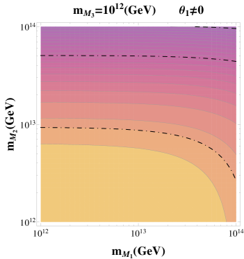
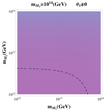
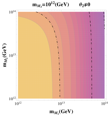
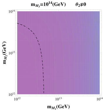
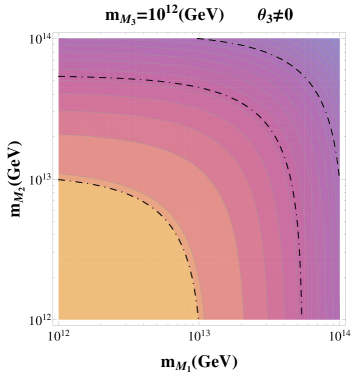
Figure 10: $\hat{\Delta}M_{h}$ contour lines in the ($m_{M_{1}}$, $m_{M_{2}}$) plane for two values of $m_{M_{3}}$ and for a single complex non vanishing $\theta_{i}$ angle. Left panels: with $m_{M_{3}}=10^{12}\,\,\mathrm{GeV}$. Right panels: with $m_{M_{3}}=10^{14}\,\,\mathrm{GeV}$. Top panels: $\theta_{1}=3\pi/4\,e^{i\pi/4}$, $\theta_{2}=\theta_{3}=0$. Middle panels: $\theta_{2}=3\pi/4\,e^{i\pi/4}$, $\theta_{1}=\theta_{3}=0$. Bottom panels: $\theta_{3}=3\pi/4\,e^{i\pi/4}$, $\theta_{1}=\theta_{2}=0$. The rest of input parameters are set to the reference values in (127).

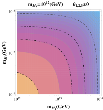
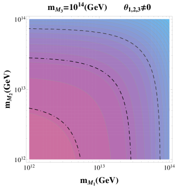
Figure 11: $\hat{\Delta}M_{h}$ contour lines in the ($m_{M_{1}}$, $m_{M_{2}}$) plane for two values of $m_{M_{3}}$ and for three non vanishing complex $\theta_{i}$ angles: $\theta_{1}=3\pi/8\,e^{i\pi/4}$, $\theta_{2}=\pi/2\,e^{i\pi/5}$ and $\theta_{3}=3\pi/4\,e^{i\pi/7}$. Left panel: $m_{M_{3}}=10^{12}\,\,\mathrm{GeV}$. Right panel: $m_{M_{3}}=10^{14}\,\,\mathrm{GeV}$. The rest of input parameters are set to the reference values in (127).

6 Conclusions

In this paper we have presented the full one-loop radiative corrections to the renormalized ${\cal CP}$-even Higgs boson self-energies and to the lightest Higgs boson mass, $M_{h}$, from the three-generations in the neutrino-sneutrino sector within the context of the MSSM-seesaw. This work extends and completes the previous calculation in the simplified one-generation case [16]. The most interesting features in this MSSM-seesaw are that the neutrinos, contrary to other fermions, are assumed to be Majorana particles, and that the origin for the light neutrino masses, again in contrast to the other fermions, are generated by means of the seesaw mechanism with the addition of heavy right handed neutrinos with large Majorana masses.

As a by-product, we have included here the complete set of Feynman rules in this MSSM-seesaw for the three-generation (s)neutrino case relevant for this work (again extending and completing Ref. [16]). This includes the vertices for the interactions of the neutrinos and sneutrinos with the Higgs sector and with the $Z$ boson. These Feynman rules have been presented in terms of all the physical masses and mixing angles of the particles involved, in particular in the mass eigen basis of the light and heavy Majorana neutrinos, as well as their light and heavy SUSY partners.

Our computation is a complete one-loop calculation in the Feynman diagrammatic approch without any simplifying assumptions. The corresponding analytical results are also presented in terms of the physical neutrinos, sneutrinos, $Z$, and Higgs bosons masses.

In particular we have discussed the renormalization of $\tan\beta$ and the wave function of the two Higgs doublets in the case of three generations of (s)neutrinos. As was discussed previously in the literature (in the one-generation case), the dependence of the prediction of $\Delta M_{h}$ on the Majorana mass scales depends strongly on the choice of the $\tan\beta$ renormalization. Various schemes have been analyzed, where each scheme exhibits advantages and disadvantages. Especially, the “modified $\overline{\mathrm{DR}}$” scheme ($\text{m}\overline{\text{DR}}$) was contrasted to other schemes, like the “more physical” OS and HM schemes and the “decoupling” scheme (DEC). The latter one leads, hence its name, to a full decoupling of the heavy Majorana mass scales in $\hat{\Delta}M_{h}$, which we confirm here for the three generations case. Regarding the comparison with the “more physical” schemes, like OS and HM, we have seen that they can lead to potentially unstable numerical behavior in certain regions of the MSSM-seesaw parameter space. Therefore the convergence of the perturbative expansion may not be ensured in the presence of heavy scales. We have also found that the use of the “more traditional” ${\overline{\text{DR}}}$ scheme is not convenient either, since there is an extremely high sensitivity to the choice of the $\mu_{\overline{\text{DR}}}$ scale. When this $\mu_{\overline{\text{DR}}}$ scale is set to the high Majorana scale, then the large logarithmic contributions disappear and one reaches a more stable result. The absence of large logarithmic contributions, $\log(m_{M_{i}}/\mu_{\overline{\text{DR}}})$, is automatically implemented in the $\text{m}\overline{\text{DR}}$ scheme. This $\text{m}\overline{\text{DR}}$ scheme, by construction not exhibiting complete decoupling behavior, leads to numerically stable predictions for $\Delta M_{h}$, gauge invariant to one-loop, while exhibiting a residual dependence of $\Delta M_{h}$ on the heavy Majorana mass scales. The analytic structure of those terms in the $\text{m}\overline{\text{DR}}$ scheme as well as in the OS and the $\overline{\mathrm{DR}}$ scheme have been derived and fully analyzed here for the three-generations case.

Finally, in order to cover several scenarios and hierarchies, in the numerical investigation we have analyzed the neutrino/sneutrino corrections to the renormalized ${\cal CP}$-even Higgs self-energies and $\Delta M_{h}$ with respect to all the involved masses and parameters: $m_{M_{i}}$, $\tan\beta$, $M_{A}$, $m_{\tilde{L}_{i}}$, $m_{\tilde{R}_{i}}$, $a_{\nu}$, $m_{\nu_{i}}$, $\theta_{i}$ and $b_{\nu}$. These analyses have been performed in the $\text{m}\overline{\text{DR}}$ scheme. A clear prescription has also been presented to pass from this scheme to the other introduced schemes (where, by definition, the DEC scheme would lead to very small effects.) We have ensured that our numerical scenarios are in agreement with experimental data by using the Casas-Ibarra parametrization of the neutrino sector and choosing the relevant values, e.g. of neutrino mass differences, according to the most recent experimental results. We have investigated both, the normal and the inverted hierarchy.

The pure gauge contributions, which are already present in the MSSM and grow with $\tan\beta$, can amount about $\Delta M_{h}\sim 150\,\,\mathrm{MeV}$, in the low $\tan\beta\sim 2$ region of interest here, i.e. about half of the current experimental uncertainty. These corrections arise from the sneutrino sector only, and thus are independent of the assumed hierarchy in the neutrino sector. The remaining contributions, $\hat{\Delta}M_{h}$, which are sensitive to the heavy neutrinos/sneutrinos via the Yukawa couplings in the $\text{m}\overline{\text{DR}}$ scheme, are larger than the pure gauge contributions in presence of very heavy scales, and are in contrast larger at the lower values of $\tan\beta$. We have studied the size of the corrections $\Delta M_{h}$ with respect to  the Majorana mass scales (where no dependence would have been found in the DEC scheme). The largest corrections are found in the degenerate case and for the largest allowed Majorana mass values. In the present work these maximum values have been set to $10^{15}\,\,\mathrm{GeV}$ in order to respect the perturbativity condition on the Yukawa couplings. In the large region of $10^{14}\,{\rm GeV}\;\raisebox{-3.00003pt}{$\stackrel{{\scriptstyle\displaystyle<}}{{\sim}}$}\;m_{M}\;\raisebox{-3.00003pt}{$\stackrel{{\scriptstyle\displaystyle<}}{{\sim}}$}\;10^{15}\,{\rm GeV}$ we find negative corrections of up to $\Delta M_{h}\sim{\cal O}(-5)\,\,\mathrm{GeV}$. We have also found that the corrections in the three generations case are generally larger than in the one generation case. Particularly, we have checked that for the degenerate Majorana masses scenario with no generation mixing, the corrections are indeed approximately three times larger. Finally, the dominant corrections in this work are found to be proportional to the square of the neutrino Dirac mass scale, specifically to $m_{D}^{\dagger}m_{D}$, and therefore they can be enhanced when complex $\theta_{i}$ parameters are taken into account. However, the above commented perturbativity requirements on the Yukawa of couplings will always restrict the size of the mass correction.

Appendix

Appendix A New Feynman rules

In this Appendix we collect the Feynman rules derived from the interaction Lagrangian terms of section 2 within the MSSM-seesaw that are relevant for the present work. They represent the interactions between the neutrinos and sneutrinos with the MSSM neutral Higgs bosons and between the neutrinos and sneutrinos with the Z gauge bosons. All the Feynman rules are written here in the physical basis. Here $c_{\mathrm{w}}\equiv\cos\theta_{W}$ and we have shortened the notation as in (2.1), i.e. $U_{ij}\equiv U_{i,j}$, $\tilde{U}_{ij}\equiv\tilde{U}_{i,j}$.

Neutrinos

Three-point couplings of two Majorana neutrinos to one MSSM Higgs boson and of two Majorana neutrinos to the Z gauge boson.

Sneutrinos

Three-point couplings of two sneutrinos to one MSSM Higgs boson and of two sneutrinos to the Z gauge boson. All the couplings not shown here vanish.

Four-point couplings of two neutrinos to two MSSM Higgs bosons and two neutrinos to two Z gauge bosons. All the couplings not shown vanish.

Conflict of Interests

The authors declare that there is no conflict of interests regarding the publication of this paper.

Acknowledgements

We thank H. Haber for helpful and clarifying discussions. The work of S.H. was supported by the Spanish MICINN’s Consolider-Ingenio 2010 Program under grant MultiDark CSD2009-00064. The work of M.H., J.H. and X.M. was partially supported by the European Union FP7 ITN INVISIBLES (Marie Curie Actions, PITN- GA-2011- 289442), by the CICYT through the project FPA2012-31880, by the Spanish Consolider-Ingenio 2010 Programme CPAN (CSD2007-00042) and by the Spanish MINECO’s “Centro de Excelencia Severo Ochoa” Programme under grant SEV-2012-0249. X. M. is also supported through the FPU grant AP-2012-6708. J. H. acknowledges financial support by the European Union through the FP7 Marie Curie Actions CIG NeuProbes (PCIG11- GA-2012-321582).

References

- [1] J. Beringer et al. [Particle Data Group], Phys. Rev. D 86 (2012) 010001, updated as pdg.lbl.gov
- [2] G. Aad et al. [ATLAS Collaboration], Phys. Lett. B 716 (2012) 1 [arXiv:1207.7214 [hep-ex]].
- [3] S. Chatrchyan et al. [CMS Collaboration], Phys. Lett. B 716 (2012) 30 [arXiv:1207.7235 [hep-ex]].
- [4] P. A. R. Ade et al. [Planck Collaboration], Astron. Astrophys. 571 (2014) A16 [arXiv:1303.5076 [astro-ph.CO]].
- [5] H. Nilles, Phys. Rept. 110 (1984) 1.
- [6] H. Haber and G. Kane, Phys. Rept. 117 (1985) 75.
- [7] R. Barbieri, Riv. Nuovo Cim. 11 (1988) 1.
- [8] P. Minkowski, Phys. Lett. B 67 (1977) 421.
- [9] M. Gell-Mann, P. Ramond and R. Slansky, “Complex Spinors and Unified Theories”, eds. P. Van. Nieuwenhuizen and D. Z. Freedman, Supergravity (North-Holland, Amsterdam, 1979), p.315 [Print-80-0576 (CERN)].
- [10] T. Yanagida, in Proceedings of the Workshop on the Unified Theory and the Baryon Number in the Universe, eds. O. Sawada and A. Sugamoto (KEK, Tsukuba, 1979), p.95.
- [11] S. L. Glashow, “The Future of Elementary Particle Physics,” NATO Sci. Ser. B 61 (1980) 687.
- [12] R. N. Mohapatra and G. Senjanović, Phys. Rev. Lett. 44 (1980) 912.
- [13] J. Schechter and J. W. F. Valle, Phys. Rev. D 22 (1980) 2227.
- [14] S. Heinemeyer, O. Stål and G. Weiglein, Phys. Lett. B 710 (2012) 201 [arXiv:1112.3026 [hep-ph]].
- [15] M. Fukugita and T. Yanagida, Phys. Lett. B 174 (1986) 45.
- [16] S. Heinemeyer, M. J. Herrero, S. Penaranda and A. M. Rodriguez-Sanchez, JHEP 1105 (2011) 063 [arXiv:1007.5512 [hep-ph]].
- [17] P. Draper and H. E. Haber, Eur. Phys. J. C 73 (2013) 2522 [arXiv:1304.6103 [hep-ph]].
- [18] J. Cao and J. M. Yang, Phys. Rev. D 71 (2005) 111701 [arXiv:hep-ph/0412315].
- [19] Y. Farzan, JHEP 0502 (2005) 025 [arXiv:hep-ph/0411358].
- [20] S. K. Kang, A. Kato, T. Morozumi and N. Yokozaki, Phys. Rev. D 81 (2010) 016011 [arXiv:0909.2484 [hep-ph]].
- [21] S. K. Kang, T. Morozumi and N. Yokozaki, JHEP 1011 (2010) 061 [arXiv:1005.1354 [hep-ph]].
-
[22]
For a general overview and selected references therein, see, for instance:
M. Raidal et al., Eur. Phys. J. C 57 (2008) 13 [arXiv:0801.1826 [hep-ph]]. - [23] F. Borzumati and A. Masiero, Phys. Rev. Lett. 57 (1986) 961.
- [24] J. Hisano, T. Moroi, K. Tobe, M. Yamaguchi and T. Yanagida, Phys. Lett. B 357 (1995) 579 [arXiv:hep-ph/9501407].
- [25] J. Hisano, T. Moroi, K. Tobe and M. Yamaguchi, Phys. Rev. D 53 (1996) 2442 [arXiv:hep-ph/9510309].
- [26] J. Ellis, J. Hisano, M. Raidal and Y. Shimizu, Phys. Rev. D 66 (2002) 115013 [arXiv:hep-ph/0206110].
- [27] E. Arganda and M. Herrero, Phys. Rev. D 73 (2006) 055003 [arXiv:hep-ph/0510405].
- [28] S. Antusch, E. Arganda, M. J. Herrero and A. M. Teixeira, JHEP 0611 (2006) 090 [arXiv:hep-ph/0607263].
- [29] E. Arganda, M. J. Herrero and A. M. Teixeira, JHEP 0710 (2007) 104 [arXiv:0707.2955 [hep-ph]].
- [30] E. Arganda, M. J. Herrero and J. Portoles, JHEP 0806 (2008) 079 [arXiv:0803.2039 [hep-ph]].
- [31] M. J. Herrero, J. Portoles and A. M. Rodriguez-Sanchez, Phys. Rev. D 80 (2009) 015023 [arXiv:0903.5151 [hep-ph]].
- [32] J. Ellis, J. Hisano, M. Raidal and Y. Shimizu, Phys. Lett. B 528 (2002) 86 [arXiv:hep-ph/0111324].
- [33] I. Masina, Nucl. Phys. B 671 (2003) 432 [arXiv:hep-ph/0304299].
- [34] Y. Farzan and M. E. Peskin, Phys. Rev. D 70 (2004) 095001 [arXiv:hep-ph/0405214].
- [35] Y. Grossman and H. Haber, Phys. Rev. Lett. 78 (1997) 3438 [arXiv:hep-ph/9702421].
- [36] A. Dedes, H. Haber and J. Rosiek, JHEP 0711 (2007) 059 [arXiv:0707.3718 [hep-ph]].
- [37] J. W. F. Valle, AIP Conf. Proc. 1200 (2010) 112 [arXiv:0911.3103 [hep-ph]].
- [38] C. Munoz, XLIth Rencontres de Moriond, La Thuile, 2006. Electronic proceeding: arXiv:0705.2007 [hep-ph].
- [39] W. Porod, J. Phys. Conf. Ser. 259 (2010) 012002 [arXiv:1010.4737 [hep-ph]].
- [40] M. Hirsch, M. A. Diaz, W. Porod, J. C. Romao and J. W. F. Valle, Phys. Rev. D 62 (2000) 113008 [Phys. Rev. D 65 (2002) 119901] [hep-ph/0004115].
- [41] R. Barbier, C. Berat, M. Besancon, M. Chemtob, A. Deandrea, E. Dudas, P. Fayet and S. Lavignac et al., Phys. Rept. 420 (2005) 1 [hep-ph/0406039].
- [42] U. Ellwanger, C. Hugonie and A. M. Teixeira, Phys. Rept. 496 (2010) 1 [arXiv:0910.1785 [hep-ph]].
- [43] D. E. Lopez-Fogliani and C. Munoz, Phys. Rev. Lett. 97 (2006) 041801 [hep-ph/0508297].
- [44] W. Wang, J. M. Yang and L. L. You, JHEP 1307 (2013) 158 [arXiv:1303.6465 [hep-ph]].
- [45] E. J. Chun, V. S. Mummidi and S. K. Vempati, Phys. Lett. B 736 (2014) 470 [arXiv:1405.5478 [hep-ph]].
- [46] A. Brignole, Phys. Lett. B 281 (1992) 284.
- [47] P. Chankowski, S. Pokorski and J. Rosiek, Phys. Lett. B 286 (1992) 307.
- [48] A. Dabelstein, Nucl. Phys. B 456 (1995) 25 [arXiv:hep-ph/9503443].
- [49] G. Degrassi, S. Heinemeyer, W. Hollik, P. Slavich and G. Weiglein, Eur. Phys. J. C 28 (2003) 133 [arXiv:hep-ph/0212020].
- [50] S. Martin, Phys. Rev. D 75 (2007) 055005 [arXiv:hep-ph/0701051].
- [51] R. V. Harlander, P. Kant, L. Mihaila and M. Steinhauser, Phys. Rev. Lett. 100 (2008) 191602 [Phys. Rev. Lett. 101 (2008) 039901] [arXiv:0803.0672 [hep-ph]].
- [52] P. Kant, R. V. Harlander, L. Mihaila and M. Steinhauser, JHEP 1008 (2010) 104 [arXiv:1005.5709 [hep-ph]].
- [53] T. Hahn, S. Heinemeyer, W. Hollik, H. Rzehak and G. Weiglein, Phys. Rev. Lett. 112 (2014) 141801 [arXiv:1312.4937 [hep-ph]].
- [54] O. Buchmueller et al., Eur. Phys. J. 74 (2014) 2809 [arXiv:1312.5233 [hep-ph]].
- [55] D. V. Forero, M. Tortola and J. W. F. Valle, Phys. Rev. D 86 (2012) 073012 [arXiv:1205.4018 [hep-ph]].
- [56] M. C. Gonzalez-Garcia, M. Maltoni, J. Salvado and T. Schwetz, JHEP 1212 (2012) 123 [arXiv:1209.3023 [hep-ph]].
- [57] F. Capozzi, G. L. Fogli, E. Lisi, A. Marrone, D. Montanino and A. Palazzo, arXiv:1312.2878 [hep-ph].
- [58] B. Pontecorvo, Sov. Phys. JETP 6 (1957) 429 [Zh. Eksp. Teor. Fiz. 33 (1957) 549].
- [59] Z. Maki, M. Nakagawa and S. Sakata, Prog. Theor. Phys. 28 (1962) 870.
- [60] J. A. Casas and A. Ibarra, Nucl. Phys. B 618 (2001) 171 [arXiv:hep-ph/0103065].
- [61] S. Heinemeyer, W. Hollik and G. Weiglein, Comput. Phys. Commun. 124 (2000) 76 [arXiv:hep-ph/9812320].
- [62] T. Hahn, S. Heinemeyer, W. Hollik, H. Rzehak and G. Weiglein, Comput. Phys. Commun. 180 (2009) 1426; see: www.feynhiggs.de .
- [63] S. Heinemeyer, W. Hollik and G. Weiglein, Eur. Phys. J. C 9 (1999) 343 [arXiv:hep-ph/9812472].
- [64] M. Frank, T. Hahn, S. Heinemeyer, W. Hollik, H. Rzehak and G. Weiglein, JHEP 0702 (2007) 047 [arXiv:hep-ph/0611326].
- [65] M. Sperling, D. Stockinger and A. Voigt, JHEP 1307 (2013) 132 [arXiv:1305.1548 [hep-ph]].
- [66] M. Frank, S. Heinemeyer, W. Hollik and G. Weiglein [arXiv:hep-ph/0202166].
- [67] A. Freitas and D. Stockinger, Phys. Rev. D 66 (2002) 095014 [arXiv:hep-ph/0205281].
- [68] P. Nason, S. Dawson and R.K. Ellis, Nucl. Phys. B 327 (1989) 49.
- [69] J. Küblbeck, M. Böhm and A. Denner, Comput. Phys. Commun. 60 (1990) 165.
- [70] A. Denner, H. Eck, O. Hahn and J. Küblbeck, Phys. Lett. B 291 (1992) 278.
- [71] A. Denner, H. Eck, O. Hahn and J. Küblbeck, Nucl. Phys. B 387 (1992) 467.
- [72] T. Hahn, Comput. Phys. Commun. 140 (2001) 418 [arXiv:hep-ph/0012260].
- [73] T. Hahn and C. Schappacher, Comput. Phys. Commun. 143 (2002) 54 [arXiv:hep-ph/0105349].
- [74] T. Fritzsche, T. Hahn, S. Heinemeyer, F. von der Pahlen, H. Rzehak and C. Schappacher, Comput. Phys. Commun. 185 1529 [arXiv:1309.1692 [hep-ph]].
- [75] T. Hahn and M. Perez-Victoria, Comput. Phys. Commun. 118 (1999) 153 [arXiv:hep-ph/9807565].
- [76] A. Denner, Fortsch. Phys. 41 (1993) 307 [arXiv:0709.1075 [hep-ph]].