Stochastic Variational Method as a Quantization Scheme II: Quantization of Electromagnetic Fields

Abstract

Quantization of electromagnetic fields is investigated in the framework of stochastic variational method (SVM). Differently from the canonical quantization, this method does not require canonical form and quantization can be performed directly from the gauge invariant Lagrangian. The gauge condition is used to choose dynamically independent variables. We verify that, in the Coulomb gauge condition, SVM result is completely equivalent to the traditional result. On the other hand, in the Lorentz gauge condition, SVM quantization can be performed without introducing the indefinite metric. The temporal and longitudinal components of the gauge filed, then, behave as c-number functionals affected by quantum fluctuation through the interaction with charged matter fields. To see further the relation between SVM and the canonical quantization, we quantize the usual gauge Lagrangian with the Fermi term and argue a stochastic process with a negative second order correlation is introduced to reproduce the indefinite metric.

I Introduction

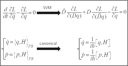
Figure 1: For quantization, the Euler-Lagrange equation is modified in SVM, while the canonical equation is changed in the canonical quantization. The mean forward and backward derivatives respectively $D$ and $\tilde{D}$ are defined in Ref. kk4 .

Stochastic variational method (SVM) is a generalized method of the variational procedure where dynamical variables are extended to the domain of stochastic ones. Instead of determining an optimal path of each stochastic process, this variational method aims to determine the optimized evolution of the probability distribution function. The method was firstly introduced by Yasue yasue to reformulate Nelson’s stochastic quantization method nelson1 ; nelson2 from the point of view of the variation principle.

Subsequently, SVM has been extended to more general cases. For example, the Navier-Stokes equation kk1 ; kk2 ; koide , the Gross-Pitaevskii equation morato ; kk2 , and the Schrödinger-Langevin (Kostin) equation misawa are formulated in SVM approach. Further aspects of SVM have also been studied, such as the Noether’s theorem misawa3 , the uncertainty relation kk3 , the applications to the many-body particle systems morato , and continuum media kk1 ; kk2 . Although many groups dav ; guerra ; zamb ; hase ; marra ; jae ; pav ; rosen ; wang ; naga ; cre ; arn ; kappen ; eyink ; gomes ; hiroshima ; serva ; yamanaka have investigated SVM, the applicability has not yet been well explored. Thus it is worth investigating the applicability of SVM to more complex systems.

In this series of works, we focus on the applicability of SVM as an alternative field quantization scheme. In Part I, we discussed the formulation of SVM to the field quantization and showed that the complex Klein-Gordon equation can be quantized appropriately and this method has an advantage for the definition of the Noether charge kk4 . This paper is Part II and we discuss the quantization of electromagnetic fields in the framework of SVM.

There is a sufficient reason to expect that the SVM quantization provides another perspective in the gauge field quantization compared to the usual canonical quantization. The canonical quantization is implemented by employing the commutation relations of canonically conjugate variables. As is well-known, however, this procedure is not straightforward for electromagnetic fields because the canonical momentum for the time component of the four-vector gauge field $A^{\mu}(x)$ vanishes. To circumvent this difficulty in a covariant manner, for example, the so-called Fermi term is introduced to the Lagrangian density, paying the price of introducing the indefinite metric (Fock state vector with a negative norm). We need to take a special care to project out the undesirable negative norm states from the physical Fock space.

Such a difficulty of the canonical formulation with dynamical constraints already appears in the classical level. Nevertheless, this does not give rise to any problem to derive the classical equations of motion by the variational procedure. Therefore, if quantization can be regarded as the stochastic generalization of the optimization of actions as is claimed in SVM, the gauge field quantization should be performed directly to the same classical action without introducing additional terms. See also Fig. 1.

The principal purposes of the present work are twofold. One is to confirm our speculation mentioned above, that is, to apply the SVM quantization to the gauge invariant Lagrangian and discuss the properties of the derived quantized dynamics. The other is to investigate the counterpart of the indefinite metric in SVM. If SVM gives the consistent framework of quantization, it will be applicable even to the usual gauge Lagrangian with the Fermi term and the well-known result should be reproduced. For this, we need to extend the concept of a stochastic process to represent the indefinite metric in SVM.

This paper is organized as follows. In Sec. II, for the sake of book-keeping, we introduce our notation for the discretization scheme of the Lagrangian density of electromagnetic fields. In Sec. III, the stochastic variation is applied to the gauge invariant Lagrangian density. In Sec. IV the application to the Lagrangian density with the Fermi term is discussed by generalizing the concept of stochastic process to reproduce the indefinite metric. Section V is devoted to concluding remarks.

II Stochastic Lagrangian Density of Electromagnetic Fields

In SVM, quantum fluctuation is introduced as random noise in a classical system. Thus, for a system of fields, the field configuration becomes not smooth in space and time. To deal with such a behavior, we introduce the space lattice discretization of the field variables as is done in kk4 . In this section, for the sake of book-keeping of notations, we summarize the scheme, extending to the vector fields.

II.1 Discretized Expression of Derivatives

For the discretization scheme, we introduce a set of $N^{3}$ cubic lattice grid points forming a cubic domain of side $L$, volume $V=L^{3}.$ The side of the unit lattice cube $\Delta x$ is $\Delta x$ $=L/N$. We denote the set of the whole lattice point by $\Omega=\left\{\mathbf{x}=(x_{l},y_{m},z_{n})=(l\Delta x,m\Delta x,n\Delta x),\ 0\leq l,m,n\leq N-1\right\}$. For a given time, spatial configuration of a field is completely specified by a set of values $f=\{f_{\mathbf{x}};\mathbf{x\in}\Omega\}$ imposing the periodic boundary condition in each direction. For this purpose, $N$ is ought to be an even integer. The periodic boundary condition is then expressed as

$$f_{\mathbf{x}}=f_{\mathbf{x}+\mathbf{e}^{i}L},$$ (1)

where $\mathbf{e}^{i}$ is defined by $\mathbf{e}^{x}=(1,0,0)$, $\mathbf{e}^{y}=(0,1,0)$ and $\mathbf{e}^{z}=(0,0,1)$. Then the spatial derivative is defined by

$$\nabla^{i}f_{\mathbf{x}}=\frac{f_{\mathbf{x}+\mathbf{e}^{i}\Delta x}-f_{\mathbf{x}-\mathbf{e}^{i}\Delta x}}{2\Delta x},$$ (2)

and the corresponding Laplacian operator is expressed as

$$\Delta_{\mathbf{x}}f_{\mathbf{x}}\equiv\sum_{i}\nabla^{i}\nabla^{i}f_{\mathbf{x}}=\sum_{i}\frac{f_{\mathbf{x}+2\mathbf{e}^{i}\Delta x}-2f_{\mathbf{x}}+f_{\mathbf{x}-2\mathbf{e}^{i}\Delta x}}{4(\Delta x)^{2}}.$$ (3)

Note that the spatial derivative here is the average of the two spatial derivatives defined Ref. kk4 . This is to simplify the introduction of the gauge conditions. We verify the partial integration formula over the whole space as in Refs. kk1 ; kk2 ; kk4 ,

$$\sum_{\mathbf{x\in\Omega}}h_{\mathbf{x}}\nabla g_{\mathbf{x}}=-\sum_{\mathbf{x\in\Omega}}g_{\mathbf{x}}\nabla h_{\mathbf{x}}$$ (4)

for any field configurations $f$ and $g$, due to the periodic boundary condition.

On the other hand, we keep the two different discretized definitions for the time derivative as,

$$(\partial_{t})_{+}f_{\mathbf{x}}(t) =\frac{f_{\mathbf{x}}(t+dt)-f_{\mathbf{x}}(t)}{dt}~{}~{}~{}~{}(dt\rightarrow 0_{+}),$$ (5a)

$$(\partial_{t})_{-}f_{\mathbf{x}}(t) =\frac{f_{\mathbf{x}}(t+dt)-f_{\mathbf{x}}(t)}{dt}~{}~{}~{}~{}(dt\rightarrow 0_{-}).$$ (5b)

These do not coincide even in the limit $\left(\left|dt\right|\rightarrow 0\right)$ in the presence of noises, as is discussed in Refs. kk2 ; kk4 . Note that SVM is formulated based on the stochastic calculus of the Wiener process and thus any higher order contribution in terms of $dt$ should be ignored. For the space direction, the infinitesimal limit of $\Delta x$ is taken in the end of calculations.

For the later convenience, we introduce the following notations,

$$(\partial_{+})_{\mu}=\left(\frac{1}{c}(\partial_{t})_{+},\nabla\right),~{}~{}~{}~{}(\partial_{-})_{\mu}=\left(\frac{1}{c}(\partial_{t})_{-},\nabla\right),$$ (6)

where $(\partial_{\pm})^{\mu}\equiv g^{\mu\nu}(\partial_{\pm})_{\nu}$, $c$ is the speed of light and $g^{\mu\nu}=diag(1,-1,-1,-1)$ is the Minkowsky metric tensor. These are just convenient notations and do not mean that these are Lorentz covariant.

II.2 Discretized Expression of Gauge Transform

Let us now introduce the gauge field in the discretized form as

$$A^{\mu}(x)=(A^{0}(\mathbf{x},t),\mathbf{A}(\mathbf{x},t))\longrightarrow A^{\mu}_{\mathbf{x}}(t)=(A^{0}_{\mathbf{x}}(t),\mathbf{A}_{\mathbf{x}}(t)).$$ (7)

From the definitions introduced in the previous subsection, the gauge transform can be expressed in two different ways;

$$A_{\mathbf{x}}^{\mu}(t)\longrightarrow(A_{\mathbf{x}}^{\prime})^{\mu}(t) =A_{\mathbf{x}}^{\mu}(t)-\partial_{+}^{\mu}\lambda_{\mathbf{x}}(t),$$ (8a)

$$A_{\mathbf{x}}^{\mu}(t)\longrightarrow(A_{\mathbf{x}}^{\prime})^{\mu}(t) =A_{\mathbf{x}}^{\mu}(t)-\partial_{-}^{\mu}\lambda_{\mathbf{x}}(t).$$ (8b)

Here $\lambda_{\mathbf{x}}(t)$ is an arbitrary smooth function in time. Therefore the above two expressions of the gauge transforms are completely equivalent since $\partial_{+}^{\mu}\lambda_{\mathbf{x}}(t)=\partial_{-}^{\mu}\lambda_{\mathbf{x}}(t)$ in the infinitesimal $\left|dt\right|$ limit as mentioned above.

Then, by applying the argument in Ref. kk4 , the discretized Lagrangian density is given by the average of the $+$ and $-$ contributions as

$$\mathcal{L}=-\frac{1}{8}F_{+}^{\mu\nu}(F_{+})_{\mu\nu}-\frac{1}{8}F_{-}^{\mu\nu}(F_{-})_{\mu\nu},$$ (9)

where

$$F_{+}^{\mu\nu} =\partial_{+}^{\mu}A^{\nu}-\partial_{+}^{\nu}A^{\mu},$$ (10a)

$$F_{-}^{\mu\nu} =\partial_{-}^{\mu}A^{\nu}-\partial_{-}^{\nu}A^{\mu}.$$ (10b)

See also Refs. kk2 ; kk3 . It should be stressed that this Lagrangian density is invariant under the gauge transforms Eq. (8a) and Eq. (8b) even for a finite spatial grid.

As is well-known, discretization scheme of the gauge field has been already formulated in terms of the link variables and widely used in the lattice field theory. In the present work, however, we will not introduce the link variable because the SVM quantization results are compared directly to that of canonical quantization of electromagnetic fields.

II.3 $\mathbf{k}-$Representation and Polarization Vector

To employ the stochastic variation, we have to specify independent degrees of freedom, to each of which independent noises are introduced. In the present case, the Lagrangian density (9) is expressed in terms of the gauge field $A^{\mu}$ which has four components, but only two of them are independent due to the gauge invariance.

For this purpose, it is natural to choose the two transverse components as the two independent variables, because the classical electromagnetic wave contains only the transverse components. The transverse component in the discretized form is defined by

$$\nabla\cdot\mathbf{A}_{\bot}=0,$$ (11)

where the subscript $\bot$ denotes the transverse component.

As was discussed in Ref. kk4 , the field quantization in SVM can be done both in the $\mathbf{x}-$ and $\mathbf{k}-$representations. The properties of the quantized electromagnetic fields is studied extensively in the momentum space. Thus, in the following, we develop SVM quantization in the $\mathbf{k}-$representation.

The field variables in the $\mathbf{k}-$representation, $A_{\mathbf{k}}^{(r)}$, is defined by the following linear transform,

$$\mathbf{A}_{\mathbf{x}}=\sqrt{\Delta^{3}\mathbf{k}}\sum_{r=1}^{3}\sum_{\mathbf{k}}\mathbf{e}_{\mathbf{k},r}A_{\mathbf{k}}^{(r)}(t)\frac{e^{i\mathbf{k\cdot x}}}{\sqrt{V}},$$ (12)

where $\Delta^{3}\mathbf{k}=(2\pi)^{3}/L^{3}$ and the three vectors $\left\{\mathbf{e}_{\mathbf{k},r},r=1,2,3\right\}$ are orthogonal unit vectors, forming an orthonormal base for each given $\mathbf{k}$. Now, we can always choose that

$$\mathbf{e}_{\mathbf{k},3}=\mathbf{q}_{\mathbf{k}}/\left|\mathbf{q}_{\mathbf{k}}\right|,\$$ (13)

where $\mathbf{q}_{\mathbf{k}}$ is the real eigenvalue of the discretized derivative operator $\nabla$ with periodic boundary conditions, satisfying

$$\nabla\ e^{i\mathbf{k\cdot x}}=i\mathbf{q}_{\mathbf{k}}\ e^{i\mathbf{k\cdot x}},$$ (14)

and expressed as

$$\mathbf{q}_{\mathbf{k}}=\frac{1}{\Delta x}(\sin(k_{x}\Delta x),\sin(k_{y}\Delta x),\sin(k_{z}\Delta x)),$$ (15)

where $\mathbf{k}=\frac{2\pi}{L}(n_{x},n_{y},n_{z})$ with $n_{i}~{}(i=x,y,z)$ being an integer satisfying $-(N-1)/2\leq n_{i}\leq(N-1)/2$. Note that, as was discussed in Ref. kk4 , $\mathbf{q}_{\mathbf{k}}$ is reduced to $\mathbf{k}$ in the continuum limit.

From the completeness of $\left\{\mathbf{e}_{\mathbf{k},r},r=1,2,3\right\}$, it is obvious that

$$\sum_{r=1,2}\mathbf{e}_{\mathbf{k},r}\mathbf{e}_{\mathbf{k},r}^{T}=I-\frac{\mathbf{q}_{\mathbf{k}}\ \mathbf{q}_{\mathbf{k}}^{T}}{\mathbf{q}_{\mathbf{k}}^{2}},$$ (16)

where $I$ is $\left(3\times 3\right)$ an identity matrix and the superscript ^T represents the transpose operation. Then the two vectors $\left\{\mathbf{e}_{\mathbf{k},r},r=1,2\right\}$ are identified as the polarization vectors. To implement the real property of the field, we use the convention normally adopted,

$$\mathbf{e}_{-\mathbf{k},r} =\mathbf{e}_{\mathbf{k},r}~{}~{}~{}~{}(r=1,2),$$ (17a)

$$\mathbf{e}_{-\mathbf{k},3} =-\mathbf{e}_{\mathbf{k},3}.$$ (17b)

In terms of these polarization vectors, the transverse field $\mathbf{A}_{\bot}$ can simply expressed as

$$\mathbf{A}_{\bot\mathbf{x}}=\sqrt{\Delta^{3}\mathbf{k}}\sum_{r=1}^{2}\sum_{\mathbf{k}}\mathbf{e}_{\mathbf{k},r}A_{\mathbf{k}}^{(r)}(t)\frac{e^{i\mathbf{k\cdot x}}}{\sqrt{V}}.$$ (18)

On the other hand, the temporal and longitudinal components $A_{\mathbf{x}}^{0}(t)$ and $\mathbf{A}_{\|\mathbf{x}}(t)$, which are not the dynamical variables in the present case, are expressed as

$$A_{\mathbf{x}}^{(0)} =\sqrt{\Delta^{3}\mathbf{k}}\sum_{\mathbf{k}}A_{\mathbf{k}}^{(0)}(t)\frac{e^{i\mathbf{k\cdot x}}}{\sqrt{V}},$$ (19)

$$\mathbf{A}_{\|\mathbf{x}} =\sqrt{\Delta^{3}\mathbf{k}}\sum_{\mathbf{k}}\mathbf{e}_{\mathbf{k},3}A_{\mathbf{k}}^{(3)}(t)\frac{e^{i\mathbf{k\cdot x}}}{\sqrt{V}}.$$ (20)

Note that our new independent variables $\left\{A_{\mathbf{k}}^{(r)}(t),A_{-\mathbf{k}}^{(r)}(t),r=1,2\right\}$ are complex but not independent, because $A_{\mathbf{k}}^{(r)\ast}(t)=A_{-\mathbf{k}}^{(r)}(t)$ because the condition that $\mathbf{A}_{\bot\mathbf{x}}$ is a real field with the convention Eq.(17a). In terms of real and imaginary parts,

$$A_{\mathbf{k}}^{(r)}(t)=\frac{R_{\mathbf{k}}^{(r)}(t)+iI_{\mathbf{k}}^{(r)}(t)}{\sqrt{2}},$$ (21)

with

$$R_{\mathbf{k}}^{(r)}(t)=R_{\mathbf{-k}}^{(r)}(t),~{}~{}~{}~{}I_{\mathbf{k}}^{(r)}(t)=-I_{\mathbf{-k}}^{(r)}(t).$$ (22)

For the sake of the later convenience, we introduce a new real variables, $\left\{\xi_{\mathbf{k}}^{(r)},r=1,2\right\}$ for any $\mathbf{k}$ from which we define the field amplitudes as

$$\xi_{\mathbf{k}}^{(r)}(t) =R_{\mathbf{k}}^{(r)}(t),$$ (23a)

$$\xi_{\mathbf{-k}}^{(r)}(t) =I_{\mathbf{k}}^{(r)}(t).$$ (23b)

III Stochastic Variation for Gauge Invariant Lagrangian

III.1 transverse components

We apply the stochastic variational method to the gauge invariant Lagrangian density (9) following Ref. kk4 .

Now we replace these fields with stochastic variables as

$$\xi_{\mathbf{k}}^{(r)}(t)\rightarrow\hat{\xi}_{\mathbf{k}}^{(r)}(t).$$ (24)

Here the symbol $\char 94\relax$ is used to express stochastic variables. The forward and backward stochastic differential equations (SDEs) are, respectively, given by

$$d\hat{\xi}_{\mathbf{k}}^{(r)}(t) =u_{\mathbf{k}}^{(r)}(\{\hat{\xi}\},t)dt+\sqrt{\frac{2\nu}{\Delta^{3}\mathbf{k}}}dW_{\mathbf{k}}^{(r)}(t)~{}~{}~{}~{}(dt>0),$$ (25a)

$$d\hat{\xi}_{\mathbf{k}}^{(r)}(t) =\tilde{u}_{\mathbf{k}}^{(r)}(\{\hat{\xi}\},t)dt+\sqrt{\frac{2\nu}{\Delta^{3}\mathbf{k}}}d\tilde{W}_{\mathbf{k}}^{(r)}(t)~{}~{}~{}~{}(dt<0).$$ (25b)

The unknown functionals $u_{\mathbf{k}}^{(r)}(\left\{{\xi}\right\},t)$ and $\tilde{u}_{\mathbf{k}}^{(r)}(\left\{{\xi}\right\},t)$ of $\left\{{\xi}\right\}=\left\{{\xi}_{\mathbf{k}}^{(r)},r=1,2,\ \forall\mathbf{k}\right\}$ are determined by the variational procedure. The noise terms $dW_{\mathbf{k}}^{(r)}(t)$ and $d\tilde{W}_{\mathbf{k}}^{(r)}(t)$ in the above are defined by the two sets of independent Wiener processes,

$$E[dW_{\mathbf{k}}^{(r)}(t)] =0,$$ (26a)

$$E[dW_{\mathbf{k}}^{(r)}(t)dW_{\mathbf{k}^{\prime}}^{(s)}(t)] =\delta_{rs}\delta_{\mathbf{k,k^{\prime}}}^{(3)}|dt|,$$ (26b)

Another one $d\tilde{W}_{\mathbf{k}}^{(r)}$ satisfies the same correlation property and all other correlations vanish.

The functional relation between $u_{\mathbf{k}}^{(r)}$ and $\tilde{u}_{\mathbf{k}}^{(r)}$ is called the consistency condition and given by

$$u_{\mathbf{k}}^{(r)}(\{{\xi}\},t)=\tilde{u}_{\mathbf{k}}^{(r)}(\{\xi\},t)+\frac{2\nu}{\Delta^{3}\mathbf{k}}\frac{\partial}{\partial{\Xi}_{\mathbf{k}}}\ln\rho(\{{\xi}\},t),$$ (27)

where $\rho$ represents the probability density of the configuration of the stochastic filed $\hat{\xi}_{\mathbf{k}}$, and defined by

$$\rho(\{\xi\},t)=E\left[\prod_{r=1}^{2}\prod_{\mathbf{k}}\delta({\xi}_{\mathbf{k}}^{(r)}-\hat{\xi}_{\mathbf{k}}^{(r)}(t))\right].$$ (28)

The dynamics of $\rho$ is obtained by the functional Fokker-Planck equation as

$$\partial_{t}\rho(\{\xi\},t)=-\sum_{r,\mathbf{k}}\frac{\partial}{\partial\xi_{\mathbf{k}}^{(r)}}(\rho(\{\xi\},t)U_{\mathbf{k}}^{(r)}(\{\xi\},t)),$$ (29)

where

$$U_{\mathbf{k}}^{(r)}(\{\xi\},t)=\frac{u_{\mathbf{k}}^{(r)}(\{\xi\},t)+\tilde{u}_{\mathbf{k}}^{(r)}(\{\xi\},t)}{2}.$$ (30)

The stochastic action which we should optimize is expressed as

$$I_{sto}=-\frac{1}{8}\int_{t_{i}}^{t_{f}}dt(\Delta^{3}\mathbf{x})\sum_{\mathbf{x}}E[\hat{F}_{+}^{\mu\nu}(\hat{F}_{+})_{\mu\nu}+\hat{F}_{-}^{\mu\nu}(\hat{F}_{-})_{\mu\nu}],$$ (31)

with $\Delta^{3}\mathbf{x}=(\Delta x)^{3}$. Here $\hat{F}_{\pm}^{\mu\nu}$ is obtained from Eq.(10a) and Eq.(10b) by substituting stochastic variables and replacing

$$(\partial_{t})_{+}\longrightarrow D,~{}~{}~{}~{}(\partial_{t})_{-}\longrightarrow\tilde{D},$$ (32)

where $D$ and $\tilde{D}$ are the mean forward and backward derivatives, respectively kk4 .

The stochastic variation for the transverse component $\hat{\xi}_{\mathbf{k}}^{(r)}$ leads to

$$\left(\partial_{t}+\sum_{r^{\prime},\mathbf{k}}U_{\mathbf{k^{\prime}}}^{(r^{\prime})}(\{\xi\},t)\frac{\partial}{\partial\xi_{\mathbf{k^{\prime}}}^{(r^{\prime})}}\right)U_{\mathbf{k}}^{(r)}(\{\xi\},t) =-\frac{1}{2}\frac{\partial}{\partial\xi_{\mathbf{k}}^{(r)}}\sum_{r^{\prime},\mathbf{k^{\prime}}}\omega_{\mathbf{k^{\prime}}}^{2}(\xi_{\mathbf{k^{\prime}}}^{(r^{\prime})})^{2}$$

$$+\frac{2\nu^{2}}{(\Delta^{3}\mathbf{k})^{2}}\frac{\partial}{\partial\xi_{\mathbf{k}}^{(r)}}\left\{\rho^{-1/2}(\{\xi\},t)\sum_{r^{\prime},\mathbf{k^{\prime}}}\left(\frac{\partial}{\partial\xi_{\mathbf{k^{\prime}}}^{(r^{\prime})}}\right)^{2}\rho^{1/2}(\{\xi\},t)\right\},$$ (33)

where $\omega_{\mathbf{k}}=c|\mathbf{q}_{\mathbf{k}}|$. The variations for the temporal and longitudinal components lead to other equations, and will be discussed in Sec. III.2.

The set of equations  (29) and (33) can be cast into the form of the functional Schrödinger equation,

$$i\hbar\partial_{t}\Psi(\{\xi\},t)=H\Psi(\{\xi\},t),$$ (34)

where

$$H=(\Delta^{3}\mathbf{k})\sum_{r,\mathbf{k}}\left[-\frac{\hbar^{2}c^{2}}{2(\Delta^{3}\mathbf{k})^{2}}\left(\frac{\partial}{\partial\xi_{\mathbf{k}}^{(r)}}\right)^{2}+\frac{1}{2c^{2}}\omega_{\mathbf{k}}^{2}(\xi_{\mathbf{k}}^{(r)})^{2}\right].$$ (35)

Here we set $\nu=\hbar c^{2}/2$. The wave functional is defined by

$$\Psi(\{\Xi\},t)=\sqrt{\rho(\{\xi\},t)}e^{i\theta(\{\Xi\},t)},$$ (36)

with the phase introduced by

$$U_{\mathbf{k}}^{(r)}(\{\xi\},t)=\frac{\hbar c^{2}}{\Delta^{3}\mathbf{k}}\frac{\partial}{\partial\xi_{\mathbf{k}}^{(r)}}\theta(\{\xi\},t).$$ (37)

All Fock state vectors are given by the stationary solutions of the functional Schrödinger equation. In particular, the vacuum state is given by

$$\Psi_{vac}(\{\xi\})=\prod_{\mathbf{k}}\sqrt{\frac{\omega_{\mathbf{k}}(\Delta^{3}\mathbf{k})}{\hbar c^{2}\pi}}e^{-(\Delta^{3}\mathbf{k})\omega_{\mathbf{k}}((\xi_{\mathbf{k}}^{(1)})^{2}+(\xi_{\mathbf{k}}^{(2)})^{2})/(2\hbar c^{2})},$$ (38)

which is normalized by one. Equivalently, by using Eq. (23), this can be expressed as a functional of $A_{\mathbf{k}}^{(r)}(t)$ as

$$\Psi_{vac}(\{R,I\})=\prod_{\mathbf{k}}\frac{\omega_{\mathbf{k}}(\Delta^{3}\mathbf{k})}{\hbar c^{2}\pi}e^{-(\Delta^{3}\mathbf{k})\omega_{\mathbf{k}}\sum_{r=1,2}((R_{\mathbf{k}}^{(r)})^{2}+(I_{\mathbf{k}}^{(r)})^{2})/(4\hbar c^{2})}.$$ (39)

It is however noted that, for example, $R_{\mathbf{k}}^{(r)}$ and $R_{\mathbf{-k}}^{(r)}$ are not independent in the expression (39).

All other stationary states of the functional Schrödinger equation are obtained by operating creation operators to this vacuum state. The creation and annihilation operators in this case are defined by

$$a_{\mathbf{k},r}+a_{\mathbf{-k},r} =l_{\mathbf{k}}R^{(r)}_{\mathbf{k}}+\frac{1}{l_{\mathbf{k}}}\frac{\partial}{\partial R^{(r)}_{\mathbf{k}}},$$ (40a)

$$a^{\dagger}_{\mathbf{k},r}+a^{\dagger}_{\mathbf{-k},r} =l_{\mathbf{k}}R^{(r)}_{\mathbf{k}}-\frac{1}{l_{\mathbf{k}}}\frac{\partial}{\partial R^{(r)}_{\mathbf{k}}},$$ (40b)

$$a_{\mathbf{k},r}-a_{\mathbf{-k},r} =i\left(l_{\mathbf{k}}I^{(r)}_{\mathbf{k}}+\frac{1}{l_{\mathbf{k}}}\frac{\partial}{\partial I^{(r)}_{\mathbf{k}}}\right),$$ (40c)

$$a^{\dagger}_{\mathbf{k},r}-a^{\dagger}_{\mathbf{-k},r} =-i\left(l_{\mathbf{k}}I^{(r)}_{\mathbf{k}}-\frac{1}{l_{\mathbf{k}}}\frac{\partial}{\partial I^{(r)}_{\mathbf{k}}}\right),$$ (40d)

where $l_{\mathbf{k}}=\sqrt{\frac{\omega_{\mathbf{k}}}{\hbar c^{2}}\Delta^{3}\mathbf{k}}$.

Using these expressions, the Hamiltonian operator can be expressed as

$$H=\sum_{r=1}^{2}\sum_{\mathbf{k}}\frac{\hbar\omega_{\mathbf{k}}}{2}(a^{\dagger}_{\mathbf{k},r}a_{\mathbf{k},r}+a_{\mathbf{k},r}a^{\dagger}_{\mathbf{k},r}).$$ (41)

Moreover, by using the definition given in Ref. kk4 , the propagator described by this functional Schrödinger equation is given by

$$\Delta^{ij}_{\bot}(x)=\frac{1}{2\pi V}\int dk^{0}\sum_{\mathbf{k}}\left(\delta_{ij}-\frac{(q_{\mathbf{k}})^{i}(q_{\mathbf{k}})^{j}}{\mathbf{q}_{\mathbf{k}}^{2}}\right)\frac{e^{-ikx}}{k^{2}+i\epsilon},$$ (42)

where $kx=k^{0}ct-\mathbf{k}\cdot\mathbf{x}$ and $k^{2}=k^{\mu}k_{\mu}=(k^{0})^{2}-\mathbf{k}^{2}$. In the continuum limit where $\mathbf{q}_{\mathbf{k}}=\mathbf{k}$, these are exactly the same as those in the canonical quantization with the Coulomb gauge condition, although we still have equations for the temporal and longitudinal components in our formulation.

For the sake of later discussion, it should be remembered that the above propagator coincides with Green’s function satisfying,

$$\left(\frac{1}{c^{2}}\partial_{t}^{2}-\Delta_{\mathbf{x}}\right)\Delta_{\bot}^{ij}(x-x^{\prime})=-\left(\delta_{ij}-\frac{\nabla_{i}\nabla_{j}}{\Delta_{\mathbf{x}}}\right)\delta^{(4)}(x-x^{\prime}).$$ (43)

III.2 temporal and longitudinal components and gauge fixing conditions

The optimized solutions of the temporal and longitudinal components are given by the variations of these components for the stochastic action (31), and we obtain

$$\left.\left[(\mathbf{e}_{\mathbf{k},3}\cdot i\mathbf{q}_{\mathbf{-k}})DA_{\mathbf{k}}^{(3)}(t)+(\mathbf{e}_{\mathbf{k},3}\cdot i\mathbf{q}_{\mathbf{-k}})\tilde{D}A_{\mathbf{k}}^{(3)}(t)+2c\mathbf{q}_{\mathbf{k}}^{2}A_{\mathbf{k}}^{(0)}(t)\right]_{\hat{\xi}=\Xi}\right. =0,$$ (44a)

$$\left.\left[(\tilde{D}D+D\tilde{D})A_{\mathbf{k}}^{(3)}(t)-c(\mathbf{e}_{\mathbf{-k},3}\cdot i\mathbf{q}_{\mathbf{k}})\tilde{D}A_{\mathbf{k}}^{(0)}(t)-c(\mathbf{e}_{\mathbf{-k},3}\cdot i\mathbf{q}_{\mathbf{k}})DA_{\mathbf{k}}^{(0)}(t)\right]_{\hat{\xi}=\Xi}\right. =0.$$ (44b)

In the present calculation, fluctuations are introduced only through the transverse components, and these two equations do not have any term depending on $\hat{\xi}_{\mathbf{k}}^{(r)}$. Thus $A_{\mathbf{x}}^{0}(t)$ and $\mathbf{A}_{\|\mathbf{x}}(t)$ are deterministic quantities. Then the mean forward and backward derivatives are, in the end, reduced to the partial time derivative and the above equations are simplified as

$$(\mathbf{e}_{\mathbf{k},3}\cdot i\mathbf{q}_{\mathbf{-k}})\partial_{t}A_{\mathbf{k}}^{(3)}(t)+c\mathbf{q}_{\mathbf{k}}^{2}A_{\mathbf{k}}^{(0)}(t) =0,$$ (45a)

$$\partial_{t}^{2}A_{\mathbf{k}}^{(3)}(t)-c(\mathbf{e}_{\mathbf{-k},3}\cdot i\mathbf{q}_{\mathbf{k}})\partial_{t}A_{\mathbf{k}}^{(0)}(t) =0.$$ (45b)

These two equations are essentially equivalent, and we need to introduce an additional condition to determine uniquely $A_{\mathbf{k}}^{(0)}$ and $A_{\mathbf{k}}^{(3)}$ as is well-known in classical electromagnetism. In the following, we consider the Coulomb and Lorentz gauge conditions.

III.2.1 Coulomb gauge

The Coulomb gauge condition $\nabla\cdot\mathbf{A}_{\mathbf{x}}(t)=0$, leads immediately to $\mathbf{A}_{\|\mathbf{x}}(t)=0$, that is,

$$A_{\mathbf{k}}^{(3)}(t)=0.$$ (46)

Substituting this result to the equations derived from the variation, we find that the temporal component also vanishes,

$$A_{\mathbf{k}}^{(0)}(t)=0.$$ (47)

That is, the temporal and longitudinal components completely disappear and we only need to consider the transverse components.

In short, the result of the canonical quantization with the Coulomb gauge condition is completely reproduced in this choice of the gauge condition.

III.2.2 Lorentz gauge

As was discussed, we can treat $A_{\mathbf{k}}^{(0)}$ and $A_{\mathbf{k}}^{3}$ are c-number fields and thus the form of the Lorentz gauge condition is well-known as

$$\partial_{t}A_{\mathbf{x}}^{0}(t)+c\nabla\cdot\mathbf{A}_{\|\mathbf{x}}(t)=0,$$ (48)

or equivalently,

$$\partial_{t}A_{\mathbf{k}}^{(0)}(t)-c(\mathbf{e}_{\mathbf{k},3}\cdot i\mathbf{q}_{\mathbf{-k}})A_{\mathbf{k}}^{(3)}(t)=0.$$ (49)

Substituting this into Eqs. (44a) and (44b), we find that the temporal and longitudinal components are, respectively, given by the solutions to the following equations,

$$(\partial_{t}^{2}+\omega_{\mathbf{k}}^{2})A_{\mathbf{k}}^{(0)}(t) =0,$$ (50a)

$$(\partial_{t}^{2}+\omega_{\mathbf{k}}^{2})A_{\mathbf{k}}^{(3)}(t) =0.$$ (50b)

Green’s functions for these c-number fields are then

$$\left(\frac{1}{c^{2}}\partial_{t}^{2}-\Delta_{\mathbf{x}}\right)\Delta^{00}(x-x\prime) =\delta^{(4)}(x-x^{\prime}),$$ (51)

$$\left(\frac{1}{c^{2}}\partial_{t}^{2}-\Delta_{\mathbf{x}}\right)\Delta_{\|}^{ij}(x-x^{\prime}) =-\frac{\nabla_{i}\nabla_{j}}{\Delta_{\mathbf{x}}}\delta^{(4)}(x-x^{\prime}).$$ (52)

Together with Eq. (42), Green’s functions are expressed in a unified way as

$$\Delta^{\mu\nu}(x-x^{\prime})=\frac{1}{(2\pi)^{4}}\int d^{4}k\frac{-g^{\mu\nu}}{k^{2}+i\epsilon}e^{-ik(x-x^{\prime})}.$$ (53)

This Green function coincides with the covariant expression of the propagator in the canonical quantization with the Lorentz gauge condition. However, differently from the case of the Coulomb gauge condition, this result is not equivalent to that of the usual canonical quantization, since the temporal and longitudinal components behave as c-number fields and are not replaced with the stochastic variables. However, the behaviors of the temporal and longitudinal components are completely changed when there is the coupling with charged matter fields, as will be shown next.

III.3 Effect of interaction

To see how the behaviors of the temporal and longitudinal components are modified by the effect of interaction, let us consider the coupling with the complex Klein-Gordon field, which is described by the following stochastic Lagrangian density,

$$\mathcal{L}_{SVM} =-\frac{1}{8}\hat{F}^{\mu\nu}_{+}(\hat{F}_{+})_{\mu\nu}-\frac{1}{8}\hat{F}^{\mu\nu}_{-}(\hat{F}_{-})_{\mu\nu}$$

$$+\frac{1}{c^{2}}\frac{(D^{\mu}_{+}\hat{\phi})^{*}((D_{+})_{\mu}\hat{\phi})+(D^{\mu}_{-}\hat{\phi})^{*}((D_{-})_{\mu}\hat{\phi})}{2}-\mu^{2}\hat{\phi}^{*}\hat{\phi},$$ (54)

where

$$D_{+}^{\mu} =(D/c-ieA^{0}/(\hbar c),-\nabla-ie\mathbf{A}/(\hbar c)),$$ (55a)

$$D_{-}^{\mu} =(\tilde{D}/c-ieA^{0}/(\hbar c),-\nabla-ie\mathbf{A}/(\hbar c)).$$ (55b)

Then, the stochastic variations of the temporal and longitudinal components respectively lead to

$$\left[\frac{1}{2}(\nabla D+\nabla\tilde{D})\cdot\mathbf{A}_{\|\mathbf{x}}(t)+c\Delta_{\mathbf{x}}A^{0}_{\mathbf{x}}(t)+\rho(\{\hat{\phi},A^{0}\})\right]_{\hat{\phi}_{R}=\phi_{R},\hat{\phi}_{I}=\phi_{I}} =0,$$ (56)

$$\left[\frac{1}{2}(\tilde{D}D+D\tilde{D})\mathbf{A}_{\|\mathbf{x}}(t)+\frac{c}{2}(\tilde{D}\nabla+D\nabla)A^{0}_{\mathbf{x}}(t)-\mathbf{J}(\{\hat{\phi},\mathbf{A}_{\|}\})\right]_{\hat{\phi}_{R}=\phi_{R},\hat{\phi}_{I}=\phi_{I}} =0.$$ (57)

where

$$\rho(\{\phi,A^{0}\}) =\frac{e}{\hbar c^{3}}\left\{\phi_{R\mathbf{x}}(t)\frac{D+\tilde{D}}{2}\phi_{I\mathbf{x}}(t)-\phi_{I\mathbf{x}}(t)\frac{D+\tilde{D}}{2}\phi_{R\mathbf{x}}(t)-\frac{e}{\hbar}A^{0}_{\mathbf{x}}(t)\sum_{i=R,I}\phi_{i\mathbf{x}}^{2}(t)\right\},$$

$$\mathbf{J}(\{\phi,\mathbf{A}_{\|}\}) =-\frac{e}{\hbar c}\left\{\phi_{R\mathbf{x}}(t)\nabla\phi_{I\mathbf{x}}(t)-\phi_{I\mathbf{x}}(t)\nabla\phi_{R\mathbf{x}}(t)+\frac{e}{\hbar c}\mathbf{A}_{\|\mathbf{x}}(t)\sum_{i=R,I}\phi_{i\mathbf{x}}^{2}(t)\right\}.$$ (58b)

Here real stochastic variables are introduced by $\hat{\phi}_{\mathbf{x}}=(\hat{\phi}_{R\mathbf{x}}+i\hat{\phi}_{I\mathbf{x}})/\sqrt{2}$, following Ref. kk4 . We can show that these $\rho$ and $\mathbf{J}$ satisfies the equation of continuity by using the stochastic Noether’s theorem.

Because now these equations depends on the stochastic variables $\hat{\phi}_{i\mathbf{x}}(t)$, the two components $A_{\mathbf{x}}^{0}(t)$ and $\mathbf{A}_{\|\mathbf{x}}(t)$ become functionals of the configuration of the complex Klein-Gordon field $\phi_{i\mathbf{x}}$. As a consequence, $D$ and $\tilde{D}$ cannot be replaced simply by the partial time derivative, but we should use the following expressions,

$$D =\left(\partial_{t}+\sum_{i=R,I}\sum_{\mathbf{x}}u_{i,\mathbf{x}}^{\phi}(\{\phi\},t)\frac{\partial}{\partial\phi_{i\mathbf{x}}}+\frac{\hbar c^{2}}{2(\Delta^{3}\mathbf{x})}\sum_{i=R,I}\sum_{\mathbf{x}}\frac{\partial^{2}}{\partial\phi_{i\mathbf{x}}^{2}}\right),$$ (59a)

$$\tilde{D} =\left(\partial_{t}+\sum_{i=R,I}\sum_{\mathbf{x}}\tilde{u}_{i,\mathbf{x}}^{\phi}(\{\phi\},t)\frac{\partial}{\partial\phi_{i\mathbf{x}}}-\frac{\hbar c^{2}}{2(\Delta^{3}\mathbf{x})}\sum_{i=R,I}\sum_{\mathbf{x}}\frac{\partial^{2}}{\partial\phi_{i\mathbf{x}}^{2}}\right),$$ (59b)

where $u_{i,\mathbf{x}}^{\phi}$ and $\tilde{u}_{i,\mathbf{x}}^{\phi}$ are, respectively, the mean forward and backward derivatives for the charged matter field $\hat{\phi}_{i\mathbf{x}}$,

$$D\hat{\phi}_{i\mathbf{x}} =u_{i,\mathbf{x}}^{\phi}(\{\hat{\phi}\},t),$$ (60a)

$$\tilde{D}\hat{\phi}_{i\mathbf{x}} =\tilde{u}_{i,\mathbf{x}}^{\phi}(\{\hat{\phi}\},t).$$ (60b)

In short, the temporal and longitudinal components are generally given by functionals of the configuration of charged matter fields whose forms are determined by the stochastic variation. When there is no charged matter, these components behave as classical fields because of the lack of the source of fluctuation, and coincide with the classical Maxwell’s equations as we have discussed.

IV Stochastic Variation for Lagrangian with Fermi Term

In this section, we apply the SVM quantization to the gauge Lagrangian with the Fermi term. This formulation in the canonical quantization is known as the method of Gupta-Bleuler, where the concept of the Fock space is extended by introducing the indefinite metric. In this section, we reproduce this result by extending the concept of a stochastic process.

The Lagrangian density is

$$\mathcal{L}=-\frac{1}{8}[F^{\mu\nu}_{+}(F_{+})_{\mu\nu}+F^{\mu\nu}_{-}(F_{-})_{\mu\nu}]-\frac{1}{4}[(\partial^{\mu}_{+}A_{\mu\mathbf{x}})^{2}+(\partial^{\mu}_{-}A_{\mu\mathbf{x}})^{2}].$$ (61)

The second term on the right hand side is the Fermi term. The variable in the $\mathbf{k}-$representation is given by $A^{(r)}_{\mathbf{k}}$ which is defined by

$$A^{\mu}=\sqrt{\Delta^{3}\mathbf{k}}\sum_{r=0}^{3}\sum_{\mathbf{k}}\varepsilon_{r\mathbf{k}}^{\mu}A^{(r)}_{\mathbf{k}}(t)\frac{e^{i\mathbf{kx}}}{\sqrt{V}}.$$ (62)

Here the covariant polarization vector $\varepsilon_{r\mathbf{k}}^{\mu}$ is defined by

$$\varepsilon_{0\mathbf{k}}^{\mu}=(1,0,0,0),~{}~{}~{}~{}\varepsilon_{r\mathbf{k}}^{\mu}=(0,\mathbf{e}_{\mathbf{k},r}),$$ (63)

and satisfies

$$\varepsilon_{r\mathbf{k}}^{\mu}(\varepsilon_{s\mathbf{k}})_{\mu} =-\zeta_{r}\delta_{rs},$$ (64a)

$$\sum_{r=0}^{3}\zeta_{r}(\varepsilon_{r\mathbf{k}}^{\mu})\varepsilon_{r\mathbf{k}}^{\nu} =-g^{\mu\nu},$$ (64b)

with $\zeta_{0}=-1$, $\zeta_{1}=\zeta_{2}=\zeta_{3}=1$.

Substituting these definitions into Eq. (61), the corresponding stochastic Lagrangian is given by

$$L_{SVM} =-\frac{(\Delta^{3}\mathbf{k})}{4c^{2}}\sum_{r,\mathbf{k}}(-\zeta_{r})E[(D\hat{\xi}^{(r)}_{\mathbf{k}}(t))^{2}+(\tilde{D}\hat{\xi}^{(r)}_{\mathbf{k}}(t))^{2}-2\omega_{\mathbf{k}}^{2}(\hat{\xi}^{(r)}_{\mathbf{k}}(t))^{2}],$$ (65)

where we have introduced the real variables as Eq. (21) for all $r$’s, and set

$$\xi^{(r)}_{\mathbf{k}}=R^{(r)}_{\mathbf{k}},~{}~{}~{}~{}\xi^{(r)}_{\mathbf{-k}}=I^{(r)}_{\mathbf{k}},~{}~{}~{}~{}(r=0,1,2,3).$$ (66)

To obtain this expression, we have dropped the term which is expressed in the form of the total time derivative by using the stochastic partial integration formula,

$$E[(D\hat{X})\hat{Y}+\hat{X}(\tilde{D}\hat{Y})]=\frac{d}{dt}E[\hat{X}\hat{Y}].$$ (67)

Differently from the previous case, the dynamics of this Lagrangian density is described by the four independent fields and hence we need to introduce four forward and backward SDEs,

$$d\hat{\xi}^{(r)}_{\mathbf{k}}(t)=u^{(r)}_{\mathbf{k}}dt+\sqrt{\frac{\hbar c^{2}}{\Delta^{3}\mathbf{k}}}dW^{(r)}_{\mathbf{k}}(t)~{}~{}~{}~{}(dt>0),$$ (68a)

$$d\hat{\xi}^{(r)}_{\mathbf{k}}(t)=\tilde{u}^{(r)}_{\mathbf{k}}dt+\sqrt{\frac{\hbar c^{2}}{\Delta^{3}\mathbf{k}}}d\tilde{W}^{(r)}_{\mathbf{k}}(t)~{}~{}~{}~{}(dt<0),$$ (68b)

where

$$E[dW^{(r)}_{\mathbf{k}}(t)] =0,$$ (69a)

$$E[dW^{(r)}_{\mathbf{k}}(t)dW^{(s)}_{\mathbf{k^{\prime}}}(t)] =\zeta_{r}\delta_{rs}\delta_{\mathbf{k,k^{\prime}}}|dt|.$$ (69b)

The correlation properties for $d\tilde{W}^{(r)}_{\mathbf{k}}$ is the same as above, but there is no correlation with $dW^{(r)}_{\mathbf{k}}$ as before.

It should be emphasized that $W^{(0)}_{\mathbf{k}}$ cannot be interpreted as the usual Wiener process, because $\zeta_{0}<0$. As far as the authors are aware, such a stochastic process is not mathematically defined, and the introduction of such a process seems to be contradict with our naive intuition. As we will show below, however, this extraordinary stochastic process corresponds to the indefinite metric in the canonical quantization. Thus, in the following, we do not discuss this mathematical consistency, but simply assume that the usual results for the Wiener process such as the Ito formula, are still applicable even for $W^{(0)}$. Or, we first assume that $\zeta_{0}$ is a positive value, and substitute $\zeta_{0}=-1$ in the last step of the calculation. Certainly, we need to understand this issue further. However, it is beyond the scope of the present exploratory study, and will be studied in the future.

Then, the corresponding Fokker-Planck equation for the density functional for the variable $\xi=\left\{\xi_{\mathbf{k}}^{(r)}\right\}$ defined before and the consistency condition are, respectively calculated as

$$\partial_{t}\rho =\sum_{r,\mathbf{k}}\frac{\partial}{\partial\xi_{\mathbf{k}}^{(r)}}\left[-u_{\mathbf{k}}^{(r)}+\zeta_{r}\frac{\nu}{\Delta^{3}\mathbf{k}}\frac{\partial}{\partial\xi_{\mathbf{k}}^{(r)}}\right]\rho=\sum_{r,\mathbf{k}}\frac{\partial}{\partial\xi_{\mathbf{k}}^{(r)}}\left[-\tilde{u}_{\mathbf{k}}^{(r)}-\zeta_{r}\frac{\nu}{\Delta^{3}\mathbf{k}}\frac{\partial}{\partial\xi_{\mathbf{k}}^{(r)}}\right]\rho,$$ (70)

$$u_{\mathbf{k}}^{(r)} =\tilde{u}_{\mathbf{k}}^{(r)}+\zeta_{r}\frac{2\nu}{\Delta^{3}\mathbf{k}}\frac{\partial}{\partial\xi_{\mathbf{k}}^{(r)}}\ln\rho,$$ (71)

where

$$\rho(\{\xi\},t)=E\left[\prod_{r=0}^{3}\prod_{\mathbf{k}}\delta(\xi_{\mathbf{k}}^{(r)}-\hat{\xi}_{\mathbf{k}}^{(r)})\right].$$ (72)

Note that, in the above results, we obtain an additional $\zeta_{r}$ factor compared to the previous calculations.

Applying the stochastic variation, we finally obtain the following functional Schödinger equation,

$$i\hbar\partial_{t}\Psi=(\Delta^{3}\mathbf{k})\sum_{r,\mathbf{k}}\zeta_{r}\left[-\frac{\hbar^{2}c^{2}}{2(\Delta^{3}\mathbf{k})^{2}}\left(\frac{\partial}{\partial\xi_{\mathbf{k}}^{(r)}}\right)^{2}+\frac{1}{2c^{2}}\omega_{\mathbf{k}}^{2}(\xi_{\mathbf{k}}^{(r)})^{2}\right]\Psi\equiv H\Psi,$$ (73)

with $\nu=\hbar c^{2}/2$. Here the wave functional is defined by $\Psi=\sqrt{\rho}e^{i\theta}$, with the phase introduced by

$$\frac{u_{\mathbf{k}}^{(r)}(\{\xi\},t)+\tilde{u}_{\mathbf{k}}^{(r)}(\{\xi\},t)}{2}=\zeta_{r}\frac{\hbar c^{2}}{\Delta^{3}\mathbf{k}}\frac{\partial}{\partial\xi_{\mathbf{k}}^{(r)}}\theta(\{\xi\},t).$$ (74)

For $r=1,2$ and $3$, this equation is essentially equivalent to the previous result (34), and hence it is already confirmed that a Fock space equivalent to the canonical quantization can be constructed. Thus, in the following, we only discuss the temporal component $r=0$.

The Fock state vector for $r=0$ is still defined by the stationary solution of the functional Schrödinger equation. The vacuum state for $r=0$ is then given by

$$\Psi_{vac}^{r=0}=N^{(0)}\prod_{\mathbf{k}}\exp{\ \left(\frac{\omega_{\mathbf{k}}\Delta^{3}\mathbf{k}}{4\hbar c^{2}}\{(R_{\mathbf{k}}^{(0)})^{2}+(I_{\mathbf{k}}^{(0)})^{2}\}\right)},$$ (75)

where $N^{(0)}$ is the normalization factor and $R_{\mathbf{k}}^{(0)}$ and $I_{\mathbf{k}}^{(0)}$ represent the real and imaginary part of $A_{\mathbf{k}}^{(0)}$, respectively as is defined in Eq. (21). Note that the state vectors constructed here is not normalizable, and to determine the normalization factor $N^{(0)}$, a certain cutoff should be introduced.

The corresponding creation and annihilation operators are defined by

$$a_{\mathbf{k},0}+a_{\mathbf{-k},0} =l_{\mathbf{k}}R_{\mathbf{k}}^{(0)}-\frac{1}{l_{\mathbf{k}}}\frac{\partial}{\partial R_{\mathbf{k}}^{(0)}},$$ (76a)

$$a_{\mathbf{k},0}^{\dagger}+a_{\mathbf{-k},0}^{\dagger} =l_{\mathbf{k}}R_{\mathbf{k}}^{(0)}+\frac{1}{l_{\mathbf{k}}}\frac{\partial}{\partial R_{\mathbf{k}}^{(0)}},$$ (76b)

$$a_{\mathbf{k},0}-a_{\mathbf{-k},0} =-i\left(l_{\mathbf{k}}I_{\mathbf{k}}^{(0)}-\frac{1}{l_{\mathbf{k}}}\frac{\partial}{\partial I_{\mathbf{k}}^{(0)}}\right),$$ (76c)

$$a_{\mathbf{k},0}^{\dagger}-a_{\mathbf{-k},0}^{\dagger} =i\left(l_{\mathbf{k}}I_{\mathbf{k}}^{(0)}+\frac{1}{l_{\mathbf{k}}}\frac{\partial}{\partial I_{\mathbf{k}}^{(0)}}\right).$$ (76d)

Then one can easily see that $a_{\mathbf{k}}\Psi_{vac}^{r=0}=0$. Thus other stationary states associated with $r=0$ are given by applying these operators to the vacuum state $\Psi_{vac}^{r=0}$.

As a result, the correlations of creation-annihilation operators introduced for this calculation are summarized as

$$[a_{\mathbf{k},r},a_{\mathbf{k}^{\prime},s}^{\dagger}]=\zeta_{r}\delta_{r,s}\delta_{\mathbf{k,k^{\prime}}},$$ (77)

and then the Hamiltonian operator is re-expressed as

$$H=\sum_{r=0}^{3}\sum_{\mathbf{k}}\zeta_{r}\frac{\hbar\omega_{\mathbf{k}}}{2}(a_{\mathbf{k},r}^{\dagger}a_{\mathbf{k},r}+a_{\mathbf{k},r}a_{\mathbf{k},r}^{\dagger}).$$ (78)

These are the well-known expressions in the canonical quantization. One can see that the norm of the state vector related to $a_{\mathbf{k},0}$ can be negative and this energy is not bounded from below, because of $\zeta_{0}=-1$. In the canonical quantization, these behaviors are interpreted as the effect of the indefinite metric. In other word, the effect of the indefinite metric can be reproduced by introducing a singular stochastic variable which has a negative second order correlation for the quantization of the temporal component in SVM.

As is well-known in the canonical quantization, this unphysical behavior is projected out from the physical state vector by requiring the condition, $(k^{0}a_{\mathbf{k},0}^{\dagger}+|\mathbf{q}_{\mathbf{k}}|a_{\mathbf{k},3}^{\dagger})\Psi_{phys}=0$.

V Concluding Remarks

In this paper, we have investigated two aspects inherent to the gauge field quantization within the framework of SVM quantization scheme.

We first investigated the applicability of the SVM field quantization to the gauge invariant Lagrangian of electromagnetic fields. We verified that the quantized dynamics obtained by the stochastic variation still has symmetry associated with the gauge transform. When the Coulomb gauge condition is employed, the result of the canonical quantization is reproduced. On the other hand, when the Lorentz gauge condition is applied, the temporal and longitudinal components of the gauge field can fluctuate only as the influence of quantized charged matter fields coupled to electromagnetic fields. This is different from the well-known result of the canonical quantization, that is, the Gupta-Bleuler formulation where the temporal and longitudinal components fluctuate even if there is no interaction. Nevertheless, the well-known propagator of the canonical quantization is still reproduced in the form of Green’s functions.

The path integral approach is considered as another quantization scheme based on the Lagrangian. In this approach, it is necessary to introduce a certain gauge fixing term to avoid infinitely many equivalent trajectories associated with the gauge symmetry. In addition, the stochastic quantization by Parisi-Wu was originally proposed as a quantization method without fixing the gauge condition, but, as pointed out in Ref. namiki , one of the gauge conditions is implicitly fixed in their formulation. Thus, to embrace our quantization in SVM, it is worth to study carefully consequences of the gauge conditions in the SVM quantization scheme from various points of view.

For this purpose, for example, the effect of the interaction with charged matter fields should be investigated in detail, although it was partly discussed in Sec. III.3. Then, we will choose one of the gauge conditions as is done in Sec. III.2. It is, however, not clear how the gauge transform is defined for quantities given by the functionals of the charged matter fields. This may correspond to the introduction of the BRST transform to the framework of SVM, which is considered to be the gauge transform for quantized systems.

At the same time, it is interesting to examine whether our result can be reproduced in the canonical quantization. Then the temporal and longitudinal components will be given by the complex functions of the operators of the transverse components. In this case, to avoid the ambiguity for the order of operators, a certain procedure such as the normal ordering product will be introduced, meanwhile, our approach do not have the ordering of variables because stochastic variables are commutable.

As for Green’s functions, Feynman’s causal boundary condition was used to derive $\Delta^{00}$ and $\Delta_{\|}^{ij}$, but the use of such a boundary condition is unusual in the classical electrodynamics. As far as the authors are aware, the same causal boundary condition is used in the absorber theory of Wheeler and Feynman, where the classical electrodynamics is re-formulated, looking for the classical origin of the infinite self-energy in Quantum Electrodynamics quantumvacuum .

We further investigated that the concept of a stochastic process is extended to reproduce the indefinite metric for the purpose of reproducing the Gupta-Bleuler formulation in SVM. This stochastic process is similar to the Wiener process, but with a negative second-order correlation. By introducing this stochastic process, we could reproduce negative norm states and unbounded energy spectra induced by the indefinite metric. We need to understand more the mathematical meaning and possibility for such an extension. This is left as a future task.

In this paper, we have discussed the Coulomb and Lorentz gauge conditions, but there are still different choices of the gauge conditions, for example, the Landau gauge condition. To deal with these conditions more systematically, it may be promising to use an auxiliary field as in the theory proposed by Nakanishi and Lautrap nakanishi . To investigate this aspect in SVM, it is necessary to develop the formulation of fermionic degrees of freedom, which is still left as an open question.

T. Koide thanks for useful comments of C. E. Aguiar about Ref. quantumvacuum . T. Koide and T. Kodama acknowledge the finantial supports from CNPq, PRONEX, and FAPERJ.  K. Tsushima is supported by the Brazilian Ministry of Science, Technology and Innovation (MCTI-Brazil), and Conselho Nacional de Desenvolvimento Científico e Tecnológico (CNPq), project 550026/2011-8.

References

- (1) K. Yasue, J. Funct. Anal. 41, 327 (1981).
- (2) E. Nelson, Phys. Rev. 150, 1079 (1966).
- (3) E. Nelson, Quantum Fluctuations, (Princeton Univ. Press, Prinston, NJ, 1985).
- (4) T. Koide and T. Kodama, arXiv:1105.6256.
- (5) T. Koide and T. Kodama, J. Phys. A: Math. Theor. 45, 255204 (2012).
- (6) T. Koide, J. Phys.: Conf. Ser. 410, 012025 (2013).
- (7) Loffredo M I and Morato L M, J. Phys. A: Math. Theor. 40 8709 (2007).
- (8) T. Misawa, Phys. Rev. A40, 3387 (1989).
- (9) T. Misawa, J. Math. Phys. 29, 2178 (1988).
- (10) T. Koide and T. Kodama, arXiv:1208.0258.
- (11) M. Davidson, Lett. Math. Phys. 3, 271 (1979).
- (12) F. Guerra and L. M. Morato, Phys. Rev. D27, 1774 (1983).
- (13) J. C. Zambrini, Int. J. Theor. Phys. 24, 277 (1985).
- (14) H. Hasegawa, Phys. Rev. D33, 2508 (1986).
- (15) R. Marra, Phys. Rev. D36, 1724 (1987).
- (16) M. Serva, Ann. Inst. Herni Poincaré, 49, 415 (1988).
- (17) M. S. Wang, Phys. Lett. A137, 437, (1989).
- (18) M. T. Jaekel, J. Phys. A23, 3497 (1990).
- (19) M. Pavon, J. Math. Phys. 36, 6774 (1995).
- (20) H. H. Rosenbrock, Proc. R. Soc. Lond. A450, 417 (1995).
- (21) M. Nagasawa, Stochastic Process in Quantum Physics, (Birkhäuser, 2000).
- (22) H. J. Kappen, Phys. Rev. Lett. 95, 200201 (2005).
- (23) D. A. Gomes, Commun. Math. Phys. 257, 227 (2005).
- (24) J. Cresson and Sébastien Darses, J. Math. Phys. 48, 072703 (2007).
- (25) G. L. Eyink, Physics D239, 1236 (2010).
- (26) M. Arnaudon and A. B. Cruzeiro, arXiv:1004.2176.
- (27) K. Kobayashi and Y. Yamanaka, Phys. Lett. A375, 3243 (2011).
- (28) F. Hiroshima, T. Ichinose and J. Lörinczi, Rev. Math. Phys. 24, 1250013 (2012).
- (29) T. Koide and T. Kodama, arXiv:1306.6922.
- (30) M. Namiki, Prog. Theor. Phys. Supp. 111, 1 (1993).
- (31) For example, see, P. W. Milonni, The Quantum Vacuum: An Introduction to Quantum Electrodynamics, (Academic Press, 1993).
- (32) See for example, N. Nakanishi, Prog. Theor. Phys. Suppl. 51, 1 (1972).