Flag flutter in inviscid channel flow

Abstract

Using nonlinear vortex-sheet simulations, we determine the region in parameter space in which a straight flag in a channel-bounded inviscid flow is unstable to flapping motions. We find that for heavier flags, greater confinement increases the size of the region of instability. For lighter flags, confinement has little influence. We then compute the stability boundaries analytically for an infinite flag, and find similar results. For the finite flag we also consider the effect of channel walls on the large-amplitude periodic flapping dynamics. We find that multiple flapping states are possible but rare at a given set of parameters, when periodic flapping occurs. As the channel walls approach the flag, its flapping amplitude decreases roughly in proportion to the near-wall distance, for both symmetric and asymmetric channels. Meanwhile, its dominant flapping frequency and mean number of deflection extrema (or “wavenumber”) increase in a nearly stepwise fashion. That is, they remain nearly unchanged over a wide range of channel spacing, but when the channel spacing is decreased below a certain value, they undergo sharp increases corresponding to a higher flapping mode.

I Introduction

A variety of experimental and theoretical studies have been conducted on the flutter of flexible plates (or “flags”) in recent years Kornecki, Dowell, and O’Brien (1976); Dowell (1980); Huang (1995); Zhang et al. (2000); Fitt and Pope (2001); Watanabe et al. (2002); Zhu and Peskin (2002); Tang, Yamamoto, and Dowell (2003); Shelley, Vandenberghe, and Zhang (2005); Argentina and Mahadevan (2005); Eloy, Souilliez, and Schouveiler (2007); Connell and Yue (2007); Eloy et al. (2008); Alben (2008a); Michelin, Smith, and Glover (2008); Manela and Howe (2009), following earlier work in the field of aeroelasticity Theodorsen (1935); Fung (1955); Bisplinghoff and Ashley (2002). Some of the more recent studies, including extensions to multiple-flag interactions and three-dimensional effects, were reviewed by Shelley and Zhang Shelley and Zhang (2011). Many of these studies addressed the stability problem: determining the region in parameter space where a flag in a uniform flow becomes unstable to transverse oscillations. Many of the studies also characterized the flag dynamics which occur after the instability grows to large-amplitude flapping, including the transitions from periodic to chaotic motions Alben and Shelley (2008); Chen et al. (2014). In most cases flag flutter was studied in flows which are unconfined or approximately so—e.g. in a flow tunnel where the tunnel walls are far from the flag. Doare et al. considered the modification to flapping due to spanwise confinement Doare, Mano, and Ludena (2011); Doare, Sauzade, and Eloy (2011). Guo and Paidoussis studied the flutter boundary for a flag confined in the direction transverse to its resting planar state Guo and Paidoussis (2000), which is also the focus of the present work. They studied plates with various combinations of clamped, pinned, and free boundary conditions at the leading and trailing edges. In the present work we focus on clamped and free boundary conditions at the leading and trailing edges, respectively, which were the most common boundary conditions employed in several recent studies Shelley and Zhang (2011). We expand on the work of Guo and Paidoussis in a few ways. First, they considered only the case of the flag support point placed symmetrically in the channel, while here we consider both symmmetric and asymmetric placement. Second, their focus was on the flutter instability boundaries. Here we compute these boundaries and also determine the large-amplitude flapping behaviors, in the presence of vortex wake dynamics. Third, we develop an infinite-flag model for which the stability boundary can be computed analytically, extending similar work from the unconfined caseShelley, Vandenberghe, and Zhang (2005); Alben (2008a) to the confined case. We also note the work of Jaiman et al. Jaiman, Parmar, and Gurugubelli (2014) which briefly considered the effects of channel walls together with fluid compressibility and viscous skin friction on the flag stability boundary.

The organization of the paper is as follows. Section II presents the model for the nonlinear dynamics of a flag in inviscid channel flow. Section III presents results for the stability boundaries and large-amplitude dynamics. Section IV specializes the model to the case of an infinite flag and presents analytical stability boundaries for various channel wall spacings. Section V presents the conclusions.

II Model

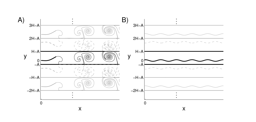
Figure 1: Examples of image systems of flags and vortex wakes that impose no-penetration boundary conditions on the channel walls at $y=-A$ and $H-A$. A) A flag (thick black line emanating from the origin) and vortex wake (thin black line emanating from the flag’s trailing edge) are shown with their images (solid and dashed gray lines). B) For the infinite flag case, a sinusoidal body is shown (thick black line) with images (solid and dashed gray lines).

We consider an inviscid model for a thin plate or flag oscillating in a flow. The model is similar to some which were described previously Alben (2009); Alben and Shelley (2008), so we will present it briefly, emphasizing the modifications needed to incorporate the channel walls. An example of a flag and vortex wake in a channel are shown in Fig. 1a. The channel is the region $-A\leq y\leq H-A$. The flag is shown as a thick black line with leading edge at the origin. The vortex wake is the thinner black line that emanates from the trailing edge of the flag and forms spirals as it evolves downstream of the flag. A uniform horizontal flow with velocity $U\mathbf{e}_{x}$ has been applied at infinity upstream, and the flag, wake, and flow evolve under a set of equations which we first summarize: Euler’s equations of fluid momentum balance; the no-penetration condition on the flag; a mechanical force balance between flag bending rigidity, inertia, and fluid pressure; Kelvin’s Circulation theorem; the Birkhoff-Rott equation for free vortex sheet dynamics; and the Kutta condition governing vorticity production at the flag’s trailing edge. We will present the most important equations here and refer to previous workAlben (2009); Saffman (1992) for the remainder and additional background information. In the following we nondimensionalize lengths by the flag length $L$, velocities by the imposed flow speed $U$, and densities by the fluid density $\rho_{f}$.

The position of the flag is described as $\zeta(s,t)=x(s,t)+iy(s,t),0\leq s\leq 1$, a curvilinear segment of length $1$ in the complex plane, parametrized by arc length $s$ and time $t$. At each instant, the flow may be computed in terms of the position and strength of a single vortex sheet in the plane. The vortex sheet has two parts: a “bound” part, coincident with the flag itself, for $0\leq s\leq 1$, and a “free” part, for $s>1$, which emanates from the flag’s trailing edge at $s=1$. On both parts, the vortex sheet’s strength is denoted $\gamma(s,t)$ and its position is denoted $\zeta(s,t)$ (the same as the flag for $0\leq s\leq 1$). On the bound sheet, the vortex sheet evolves to satisfy the no-penetration condition on the flag (but not the no-slip condition, since the flow is inviscid):

$$\mbox{Im}\left(e^{-i\theta(s,t)}\,\partial_{t}\zeta(s,t)\right) =\mbox{Im}\left(e^{-i\theta(s,t)}\,\left(1+~{}P\int_{0}^{L_{w}}~{}\gamma(s^{\prime},t)\overline{K(s,s^{\prime},t)}\,ds^{\prime}\right)\right),\;0\leq s\leq 1.$$ (1)

This condition sets the component of the body’s velocity normal to the body equal to the same component of the flow velocity. Here $\theta(s,t)$ is the tangent angle to the body. The unity term on the right hand side is the uniform background flow and $K(s,s^{\prime},t)$ is the complex flow velocity at $\zeta(s,t)$ due to a periodic array of point vortices of strength unity located at $\zeta(s^{\prime},t)+2inH,n=0,\pm 1,\pm 2,\ldots$ as well as a periodic array of point vortices of strength negative unity located at $\overline{\zeta(s^{\prime},t)}-2iA+2inH,n=0,\pm 1,\pm 2,\ldots$. Together the two arrays give the flow in the channel due to a point vortex at $\zeta(s^{\prime},t)$, enforcing the no-penetration conditions on the channel walls by the “method of images” Saffman (1992). The special integral symbol in (1) denotes a principal-value integral, due to the $\sim 1/(s-s^{\prime})$ singularity in $K(s,s^{\prime},t)$. The kernel is given by

$$K(s,s^{\prime},t)= \frac{1}{4H}\coth\left(\frac{\pi(\zeta(s,t)-\zeta(s^{\prime},t))}{2H}\right)$$

$$-\frac{1}{4H}\coth\left(\frac{\pi\left(\zeta(s,t)-\overline{\zeta(s^{\prime},t)}+2iA\right)}{2H}\right),\;0\leq s,s^{\prime}\leq 1.$$ (2)

We use a regularized version of the kernel on the free vortex sheet ($s^{\prime}>1$), which allows for smooth vortex sheet dynamics, analogous to Krasny’s method Krasny (1986):

$$K(s,s^{\prime},t)=\frac{1}{8H}\frac{\displaystyle\sinh\left(\frac{\pi}{H}(x(s,t)-x(s^{\prime},t))\right)-i\sin\left(\frac{\pi}{H}(y(s,t)-y(s^{\prime},t))\right)}{\displaystyle\sinh^{2}\left(\frac{\pi}{H}(x(s,t)-x(s^{\prime},t))\right)+\sin^{2}\left(\frac{\pi}{H}(y(s,t)-y(s^{\prime},t))\right)+\left(\frac{\pi\delta(s^{\prime},t)}{2H}\right)^{2}}$$

$$-\frac{1}{8H}\frac{\displaystyle\sinh\left(\frac{\pi}{H}(x(s,t)-x(s^{\prime},t))\right)-i\sin\left(\frac{\pi}{H}(y(s,t)+y(s^{\prime},t)+2A)\right)}{\displaystyle\sinh^{2}\left(\frac{\pi}{H}(x(s,t)-x(s^{\prime},t))\right)+\sin^{2}\left(\frac{\pi}{H}(y(s,t)+y(s^{\prime},t)+2A)\right)+\left(\frac{\pi\delta(s^{\prime},t)}{2H}\right)^{2}},$$

$$0\leq s\leq 1,\;1<s^{\prime}.$$ (3)

We set

$$\delta(s^{\prime},t)=\delta_{0}\left(1-e^{\displaystyle-|\zeta(1,t)-\zeta(s^{\prime},t))|^{2}/4\delta_{0}^{2}}\right)$$ (4)

with $\delta_{0}$ = 0.2. This regularization tapers to zero at the trailing edge $s^{\prime}=1$, so $K(s,s^{\prime},t)$ is continuous there. In other words, as $\delta(s^{\prime},t)\to 0$, the expression in (3) tends to that in (2). The tapered regularization allows for smooth vortex sheet dynamics away from the trailing edge while decreasing the effect of regularization on the generation of vorticity at the trailing edge Alben (2010). At the trailing edge, the vortex sheet is advected away from the body by the uniform background flow, so it remains in the less regularized region near $s^{\prime}=1$ for a time which is too short to allow chaotic dynamics to develop.

The vortex sheet strength $\gamma(s,t)$ is coupled to the pressure jump $[p](s,t)$ across the flag using a version of the unsteady Bernoulli equationHou, Lowengrub, and Shelley (2001); Alben (2012):

$$\partial_{t}\gamma(s,t)+\partial_{s}\left((\mu(s,t)-\tau(s,t))\gamma(s,t)\right)=\partial_{s}[p](s,t),\;0\leq s\leq 1.$$ (5)

Here $\mu(s,t)$ is the component of the flow velocity tangent to the body,

$$\mu(s,t)=\mbox{Re}\left(e^{-i\theta(s,t)}\,\left(1+~{}P\int_{0}^{L_{w}}~{}\gamma(s^{\prime},t)\overline{K(s,s^{\prime},t)}\,ds^{\prime}\right)\right)$$ (6)

and $\tau(s,t)$ is the body’s velocity component tangent to itself:

$$\tau(s,t)=\mbox{Re}\left(e^{-i\theta(s,t)}\partial_{t}\zeta(s,t)\right).$$ (7)

The unsteady Euler-Bernoulli beam equation couples the pressure loading to body inertia and bending rigidity (for a uniform beam here):

$$R_{1}\partial_{tt}\zeta+R_{2}\partial_{s}\left(\partial_{s}\kappa(s,t)ie^{i\theta(s,t)}\right)-\partial_{s}\left(T(s,t)e^{i\theta(s,t)}\right)=-[p]ie^{i\theta(s,t)}.$$ (8)

Here $R_{1}$ and $R_{2}$ are the dimensionless material parameters for the flag:

$$R_{1}=\frac{\rho_{s}h}{\rho_{f}L}\;,\;R_{2}=\frac{B}{\rho_{f}U^{2}L^{3}W}$$ (9)

Here $\rho_{s}$ is the mass per unit volume of the flag and $h$ is its thickness. We assume that $h/L$ is small, but $\rho_{s}/\rho_{f}$ may be large, so $R_{1}$ may assume any nonnegative value. As stated previously, $\rho_{f}$ is the mass per unit volume of the fluid and $L$ is the flag length. $B$ is the flag bending rigidity, $U$ is the uniform background flow speed, and $W$ is the out-of-plane width of the beam. The flow is assumed to be a 2D flow, so it is uniform in the out-of-plane direction. In (8), $\kappa=\partial_{s}\theta$ is the beam’s curvature and $T(s,t)$ is the tension in the beam, arising from its inextensibility. $T$ is eliminated in favor of $\kappa$ by integrating the tangential component of (8) from the free end of the beam ($s=1$) where $T=0$ (and $\kappa=\partial_{s}\kappa=0$). The normal component of (8) is then used to relate $[p]$ to the beam shape and motion given by $\zeta$ and $\kappa$, with “clamp” boundary conditions described below. Further details are given in a previous workAlben (2009). We also refer the reader to this work for information on how the vorticity in the free vortex sheet is generated at the trailing edge using the Kutta condition, and advected downstream using the Birkhoff-Rott equation. In the Results sections, we use the total circulation in the free vortex sheet as an indicator of the type of dynamics (periodic, chaotic, etc.). The total circulation is

$$\Gamma(t)=\int_{1}^{L_{w}}\gamma(s,t)\,ds.$$ (10)

We evolve the flag and flow using the equations just presented, as an initial-boundary-value-problem, with the flag starting in the horizontal state with uniform flow velocity $U\mathbf{e}_{x}$ at $t=0$. The upstream edge of the flag ($s=0$) is held fixed at the origin ($\zeta(0,t)=0$), and its tangent angle is perturbed from horizontal sufficiently smoothly that accelerations are continuous at $t=0$:

$$\theta(0,t)=\theta_{0}t^{3}e^{-t^{3}}\;,\;t\geq 0.$$ (11)

In the simulations we use two different perturbation magnitudes, $\theta_{0}=0.005$ and 0.1. We then compute the flag and flow for $t\geq 0$. For some parameters, as $t$ exceeds 1 the flag deflection decays exponentially with time, and tends to a flat, horizontal state, which is then considered to be a stable equilibrium. For other parameters, the flag deflection grows exponentially with time, in which case the flat state is considered to be unstable. The perturbation (11) decays rapidly for $t>1$, so it provides an initial perturbation and does not apply significant forcing to the flag at later times ($t\gg 1$) which are our focus here.

In the following sections, we determine where in the parameter space the horizontal flag is unstable. When it is unstable, we characterize the large-amplitude dynamics of the flag (amplitude, dominant frequency, and typical wavenumber), and how they depend on the parameters.

III Finite flag results

We find that for most values of $R_{1}$, $R_{2}$, $A/L$, and $A/H$, the two perturbations ($\theta_{0}=0.005$ and 0.1) lead to the same flapping state once the perturbation reaches an order-one magnitude. This is particularly true when the flapping state is periodic with a single dominant frequency. For smaller values of $R_{2}$, chaotic flapping occurs with a broadband frequency spectrum, and it is difficult to precisely define the final flapping state. For simplicity we focus on periodic flapping states.

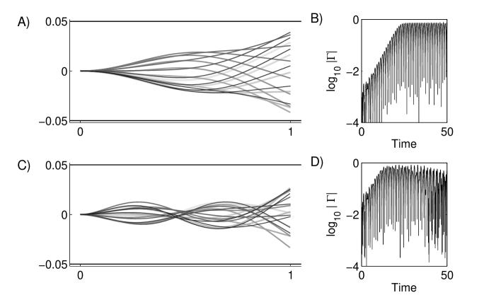
Figure 2: Examples of different flapping states which are obtained at the same parameter values but with different initial perturbations. For a smaller perturbation, $\theta_{0}(t)=0.005\,t^{3}e^{-t^{3}}$, flag snapshots (A) and total wake circulation versus time (B) are shown. For a larger perturbation $\theta_{0}(t)=0.1\,t^{3}e^{-t^{3}}$, the corresponding results are shown in (C) and (D). For both cases, $R_{1}=2.11$, $R_{2}=0.0395$, $A/L=0.05$, and $A/H=0.5$. For A and B, the channel walls are plotted with solid black lines. Note that the axes are not to scale.

In figure 2, we present an example in which our two differently-sized initial perturbations lead to apparently different flapping states, for a flag in a symmetric channel ($A/H=0.5$) of fairly small width ($A/L=0.05$). The eventual flapping state for the smaller perturbation, shown in panel a, is periodic with a single dominant frequency. The magnitude of the total wake circulation $|\Gamma|$, plotted in panel b, rises exponentially in time before saturating as a periodic oscillation. The larger initial perturbation leads to a higher wavenumber flapping mode, shown in panel c. The flapping is also much less regular, and the dominant frequency is less dominant. This can be seen qualitatively by comparing the flapping dynamics (panel c) and circulation dynamics (panel d) with the quasi-periodic case (panels a and b).

We now proceed to characterize the finite flag’s dynamics across parameter space. As noted above, in most cases of periodic flapping, the same flapping state is obtained with different initial perturbations. This is consistent with the observation of a very small range of hysteresis and bistability (about 1–2% in $R_{2}$) in a previous study of the unbounded flapping flag Alben and Shelley (2008). Therefore, for simplicity we proceed using the perturbation $\theta_{0}=0.1$ only, and focus on the periodic states which arise with this perturbation, which are almost always the same as those which arise with the perturbation $\theta_{0}=0.005$.

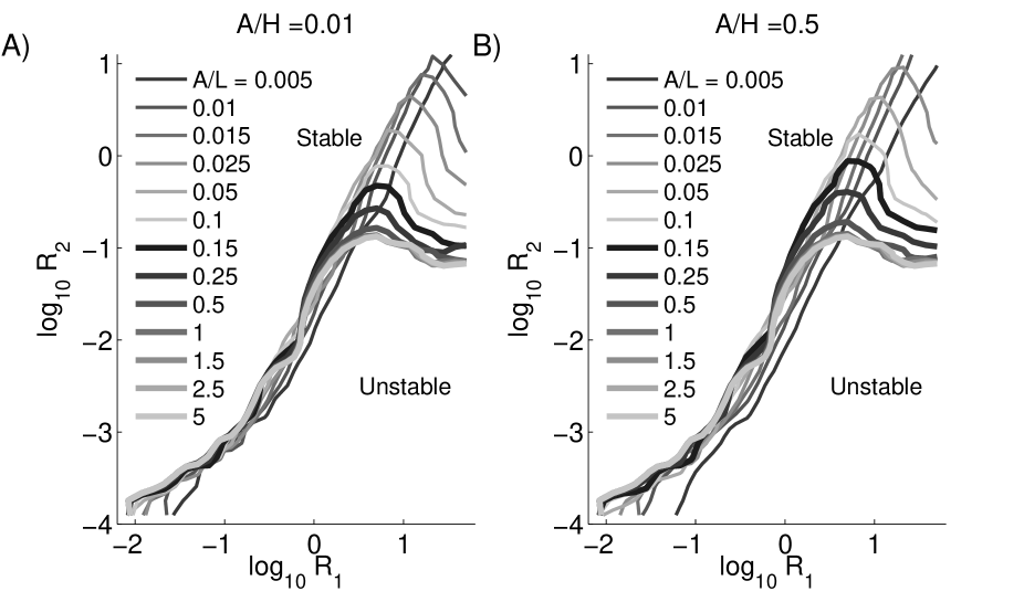
Figure 3: Stability boundaries for finite flags in the space of dimensionless flag inertia ($R_{1}$) and bending rigidity ($R_{2}$). Boundaries are shown for various ratios of near-wall-distance to flag length $A/L$ (labeled) when the far wall is much farther away ($A/H=0.01$, panel a) and when the two walls are equidistant ($A/H=0.5$, panel b).

We begin by computing the stability boundaries for the finite flag in the $R_{1}$-$R_{2}$ plane. We compute the growth (or decay) rates of the initial perturbation from data analogous to those in Fig. 2b, on a 33-by-33 grid of values in $R_{1}$-$R_{2}$ space spanning several decades in each parameter. We interpolate these values to find the location of the line with zero growth rate, which is the stability boundary. We compute the stability boundaries for two different values of $A/H$, 0.01 (shown in Fig. 3a), for which the far wall is 99 times as distant as the near wall, and 0.5 (shown in Fig. 3b), for a symmetric channel. In each panel, the stability boundaries are given for twelve different values of near-wall-distance ($A/L$) ranging from 0.005 to 5 (labeled), and plotted with different shades of gray and line thicknesses.

For the larger $A/L$ (1.5, 2.5, and 5), we find good convergence to the stability boundary for the unbounded case in panels a and b. As $A/L$ decreases, the “plateau” portion of the stability boundary moves upwards, towards larger $R_{1}$ and $R_{2}$, and becomes more curved. At smaller $R_{2}$, the stability boundary shifts slightly rightward, towards larger $R_{1}$, mainly at very small values of $A/L$. The main difference between panels a and b is that the shifts are somewhat greater in panel b, consistent with an increased instability due to increased confinement.

We now consider the large-amplitude flapping dynamics, and use three quantities to characterize them. One is the frequency, defined as the maximum frequency in the power spectrum, computed using Welch’s method Welch (1967). We compute the power spectrum from a plot of the circulation versus time, after the first time at which the circulation magnitude has reached 95% of its global maximum up to $t=50$ (in units of $L/U$). We present frequency (and other) data for cases in which the magnitude of the dominant frequency peak is at least 10 times that of the second highest peak, so that a dominant frequency can be identified clearly. The second quantity is the amplitude, defined as the largest vertical deflection of the flag over the time over which the power spectrum is computed. The third quantity is the time-averaged number of local extrema in vertical position along the flag, computed with the same temporal data as the preceding quantities. This third quantity gives a measure of the “waviness” of the flag, and is proportional to the wavenumber for a sinusoidal flag shape.

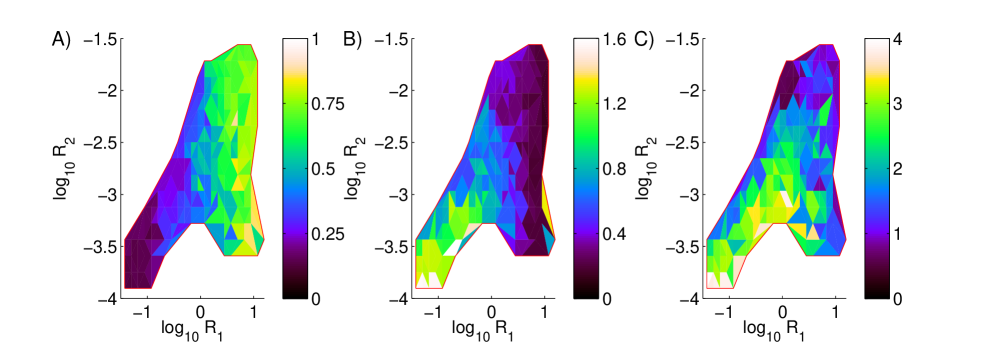
Figure 4: Flapping amplitude (A), dominant frequency (B), and time-averaged number of extrema in flag deflection (C), for an unbounded flag, in the space of dimensionless flag inertia ($R_{1}$) and bending rigidity ($R_{2}$).

Before considering the effects of channel boundedness, we plot in Fig. 4 the flapping amplitude (panel a), frequency (b), and time-averaged number of extrema (c) for the unbounded case, in the $R_{1}$-$R_{2}$ plane. This provides a baseline for comparison with the channel-bounded cases. We focus on the region where reliable frequency data can be obtained. This is the region outlined in red in panels a, b, and c. Above and to the left of this region, the straight state is stable and no flapping occurs. To the right of this region, the flag inertia $R_{1}$ is so large that simulations take a very long time to converge to a stable quasi-periodic state. Below this region, the flapping is too chaotic to have a clear definition of a dominant frequency. Nonetheless, the red region covers a large portion of the space of flapping states, and certain basic trends can be seen.

In panel a, we see that the amplitude increases with increasing $R_{1}$. Larger flag inertia results in larger flag momentum. The flag is able to maintain its momentum for longer times against fluid forces, and moves farther before reversing direction. The amplitude does not vary as strongly with bending rigidity ($R_{2}$). In panel b, we see that the dominant frequency decreases with increasing flag inertia. This is again because the flag maintains its momentum for longer times, increasing the flapping period and decreasing the frequency. The frequency also decreases with increasing bending rigidity. Bending rigidity also resists rapid changes in flag position under changing fluid forces. This trend is opposite to that for a beam oscillating in a vacuum, so clearly fluid forces play an essential role. In panel c, we see that the average number of maximum deflections along the flag increases as the flag becomes more flexible ($R_{2}$ decreases), as expected—a more flexible flag adopts a “wavier” shape. At a given $R_{2}$, the number of maxima first increases, then decreases as $R_{1}$ increases. This behavior does not have an explanation which is obvious to us.

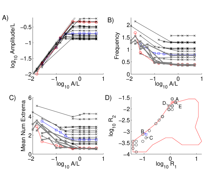
Figure 5: Flapping amplitudes (A), dominant frequencies (B), and time-averaged numbers of extrema in flag deflection (C) for flags in symmetric channels ($A/H=0.5$) with various wall spacings ($A/L$, shown on horizontal axes). The crosses connected by a given line correspond to a given $(R_{1},R_{2})$ pair. These are not labeled individually but the ensemble of values is shown by circles (and other symbols) in panel D. For five values with labels A-E, flag snapshots are shown in the panels of figure 6 with corresponding labels.

Having described how some of the basic quantities of the flapping state—amplitude, frequency, and number of deflection extrema—vary with $R_{1}$ and $R_{2}$ in the unbounded state, we now consider how these quantities vary with the channel geometry parameters, $A/L$ and $A/H$. First we consider the symmetric channel ($A/H=0.5$). We identify a set of $(R_{1},R_{2})$ which have a dominant flapping frequency across a wide range of $A/L$. These values of $(R_{1},R_{2})$ are shown by circles in Fig. 6d. For each such $(R_{1},R_{2})$, we plot the flapping amplitude (panel a), frequency (panel b) and average number of extrema (panel c). In each of the panels a–c, values for a given $(R_{1},R_{2})$ are a set of crosses connected by a solid line. We do not label each line by its value of $(R_{1},R_{2})$ to prevent visual clutter, and also because we are mainly interested in the trends which are common across the set of plots.

First, we consider the flapping amplitude (panel a). For most values of $(R_{1},R_{2})$, the behavior is as follows. Starting at the right side of the panel, where each line has its unbounded value (described in figure 4) at large $A/L$, we move to the left, in the direction of decreasing $A/L$. In most cases the amplitudes are nearly unchanged (but with a slight increase, evidence of attraction to the walls) until $A$ decreases to about the size of the amplitude in the unbounded case. Then the amplitude is forced to become at least as small as $A$. In this regime, the amplitude is usually quite close to $A$, its upper limit. But in some cases it is significantly less, so the flag remains well away from the walls. Meanwhile, the frequency (panel b) increases as the walls move towards the flag. In several cases the increase occurs as a jump separating approximate “plateau” regions. These cases are plotted with thick gray lines in panel b, with $(R_{1},R_{2})$ shown as thick gray circles in panel d. As the frequency increases, so does the mean number of deflection extrema (panel c), showing that the flag adopts a “wavier” shape as the walls move inward. The thick gray lines correspond to those for the frequency (panel b), showing that the mean numbers of extrema also undergo jumps, and remain close to certain values over a range of $A/L$. In panel d, five $(R_{1},R_{2})$ values are labeled with letters A-E. These refer to the panels in Fig. 6, in which we show sequences of snapshots at these selected $(R_{1},R_{2})$ values.

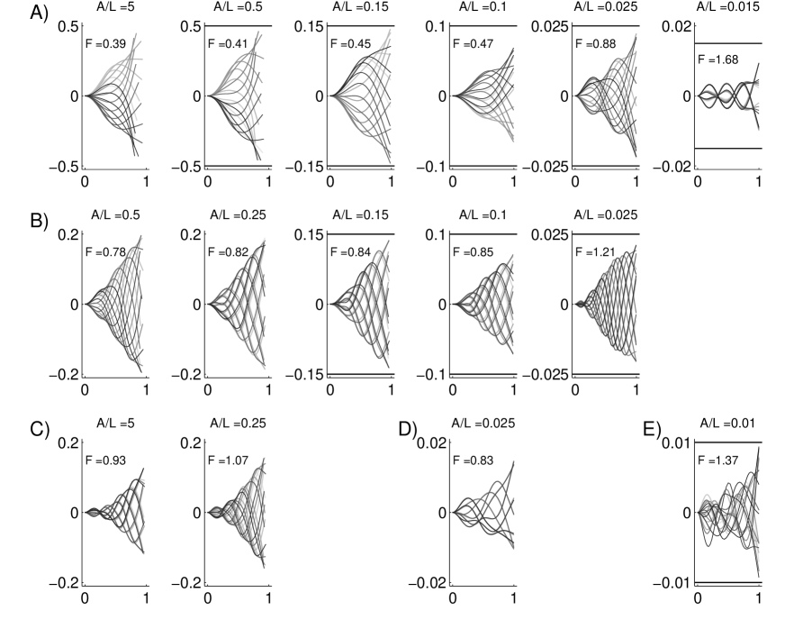
Figure 6: Snapshots for flags with fixed values of $R_{1}$ and $R_{2}$ in symmetric channels ($A/H=0.5$) of varying half-width ($A/L$). Each of the panels A-E corresponds to a different pair of $R_{1}$ and $R_{2}$, labeled in figure 5D. Within each panel, a frame shows flag snapshots at a particular $A/L$ (labeled). The axes have different scales. The dominant flapping frequencies are labeled F.

Fig. 6a shows a typical sequence of flapping states as $A/L$ decreases for fixed flag and flow parameters ($R_{1}$ and $R_{2}$). In each panel the flapping frequency is listed, denoted by F. First, at $A/L=5$, the state is essentially the unbounded case. In the next frame (moving to the right), $A/L=0.5$, so the walls are now quite close to the flag. The flag motion is nearly unchanged, however, with only a slight increase in amplitude. This slight “wall attraction” occurs at various $(R_{1},R_{2})$. Moving again to the right ($A/L=0.15$), the flag continues to flap with nearly the same shape, but with a much smaller amplitude, enforced by the walls. It is almost as though the flapping motion has simply been scaled down in the vertical direction. The flapping frequency is also nearly the same. In the next frame ($A/L=0.1$), the shape and frequency are again nearly the same, but the amplitude has decreased again. Interestingly, the flag is farther from the walls in a relative sense than in the previous panels, even though the degree of confinement is now greater. Moving to the next panel ($A/L=0.025$), the flag finally undergoes a large change in shape and in frequency (which is nearly double the previous value). The flag has transitioned to a very different flapping state. Another large transition occurs in the next frame ($A/L=0.015$), where the frequency nearly doubles again and the number of extrema also increases. Relative to the channel width, the flag is now farther from the channel wall than in the previous panel. The data corresponding to case A are shown by red circles in the panels of Fig. 5.

Moving to panel b, the second row of Fig. 6, $R_{1}$ and $R_{2}$ (labeled ‘B’ in Fig. 5d) are now reduced by about a factor of 10. In the unbounded state, similar to the first frame, the flag shows a higher bending mode than in panel a, and a higher frequency. As $A/L$ is decreased to 0.25, there is essentially no change in the flapping state. As $A/L$ is decreased again to 0.15 and to 0.1, the flapping amplitude drops twice to fit within the successively smaller channels, but the flag shapes and frequencies are only slightly changed. In the last frame ($A/L=0.025$), the flag has moved to a higher bending mode with a higher frequency. The data corresponding to case B are shown by blue squares in the panels of Fig. 5.

Panel c shows, at a nearby value of $(R_{1},R_{2})$, another example of the slight increase in flapping amplitude which can occur when the channel walls move closer to the flag. The first frame ($A/L=5$) is representative of the unbounded state. In the second ($A/L=0.25$), the walls are closer to the flag, and it has a small but noticeable increase in amplitude. Panel d shows an example of an asymmetric periodic state which occurs even though the channel is symmetric. Such asymmetric states are common in chaotic flapping, for which an example is shown in panel e, but are rare for periodic flapping in the symmetric channel.

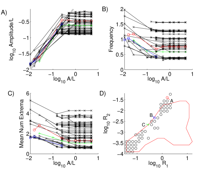
Figure 7: Flapping amplitudes (A), dominant frequencies (B), and time-averaged numbers of extrema in flag deflection (C) with various near-wall-spacings ($A/L$, shown on horizontal axes), when the far wall is much farther away ($0.01\leq A/H\leq 0.1$). The crosses connected by a given line correspond to a given $(R_{1},R_{2})$ pair. These are not labeled individually but the ensemble of values is shown by circles (and other markers) in panel D. For three values with labels A-C, flag snapshots are shown in the panels of figure 8 with corresponding labels. Data for case A are shown with red circles, for B with blue squares, and for C with green plusses.

So far we have considered the large-amplitude dynamics of flags in symmetric channels. We now look at the same results for flags when one channel wall is much closer to the flag than the other. In Fig. 7, we show the flapping amplitudes (a), frequencies (b) and mean numbers of deflection extrema (c) for an ensemble of flags with $0.01\leq A/H\leq 0.1$, so the near wall is a factor of 9–99 closer to the flag’s leading edge than the far wall. Once $A/H$ drops below 0.1, the results vary only slightly (by three percent or less) with $A/H$. The trends are similar to those in the symmetric case, with a few minor differences. In panel a, as $A/L$ decreases (so the near wall gets nearer), the flapping amplitudes undergo a larger increase before they begin to decrease. The reason is that the flags are mainly confined on one side, so they may adopt an asymmetric flapping mode which flaps with larger amplitude on the less constrained side. For this reason, the amplitude now exceeds $A/L$ in most cases when $A/L$ becomes small. However, the amplitude still scales approximately as $A/L$, meaning that the degree of asymmetry in the vertical displacement remains bounded. Although the flag could move to a much greater distance in the far-wall direction, in most cases its maximum displacement in that direction is less than 50% greater than its maximum displacement in the near-wall direction. One might have expected the flag to flap closer to the near wall than away from it in some cases, in light of the slight wall attraction we observed in the symmetric case. We have not observed such a case. If it occurs, it probably occurs only slightly and only for a small range of $A/L$. In panel d, we again mark the $(R_{1},R_{2})$ values corresponding to the data presented. Three points are labeled A–C, and these refer to the panels in Fig. 8 where the corresponding snapshots are presented. In the panels of Fig. 7, the data for case A are shown with red circles, for B with blue squares, and for C with green plusses. Cases A and B are examples in which the frequencies and mean numbers of extrema show patterns of jumping from one distinct mode to another, as in the symmetric cases.

Snapshots for case A are shown in Fig. 8a. The flapping is only slightly asymmetrical in the first frame ($A/L=0.25$), even though the flag nearly touches the near wall. In the second frame ($A/L=0.015$), the flag has moved to a clearly asymmetrical mode, with the frequency nearly doubled. In the third frame ($A/L=0.01$), the mode and frequency are nearly the same, but the amplitude is smaller. For case B (panel b), the first two frames ($A/L=0.5$ and 0.25) show a similar flapping mode with similar frequencies, although the second is more irregular (or chaotic) in frequency space. The third frame ($A/L=0.025$) shows a switch to a different mode and frequency. The flapping is however more periodic and less chaotic than in the second frame. In the fourth frame ($A/L=0.015$), the mode and frequency are similar to those in the third, but now the flapping is more chaotic. This alternating pattern of regular and chaotic flapping has been seen at other $(R_{1},R_{2})$ as the walls become closer. For case C (panel c), the first two frames ($A/L=0.25$ and 0.1) show essentially the same mode and frequency, though the amplitudes are very different. Both motions are quite symmetrical despite the large channel asymmetry. The third frame ($A/L=0.025$) has a higher frequency and number of extrema, and the degree of asymmetry is only slightly increased.

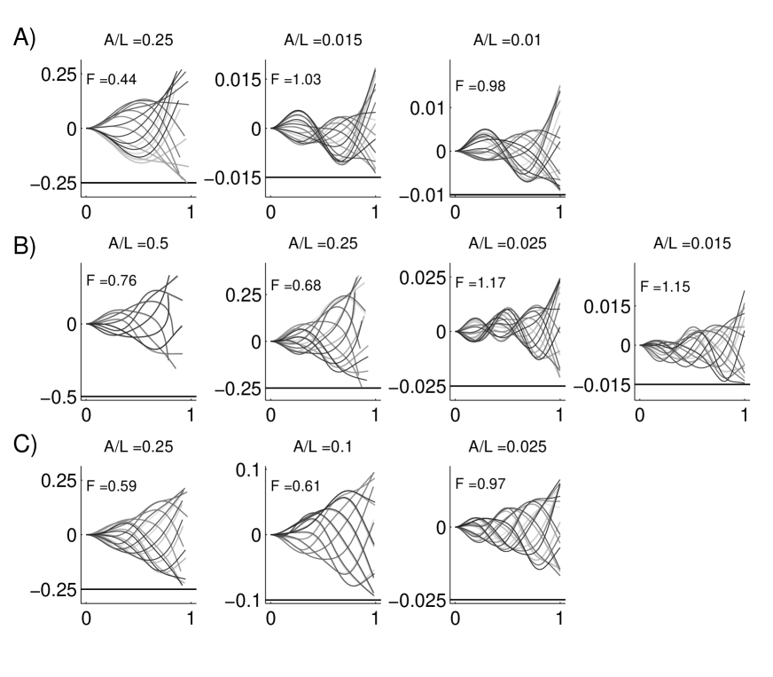
Figure 8: Snapshots for flags with fixed values of $R_{1}$ and $R_{2}$ with various near-wall-spacings ($A/L$), when the far wall is much farther away ($0.01\leq A/H\leq 0.1$). Each of the panels a–c corresponds to a different pair of $R_{1}$ and $R_{2}$, labeled in figure 7d. Within each panel, a frame shows flag snapshots at a particular $A/L$ (labeled). The axes have different scales. The dominant flapping frequencies are labeled F.

IV Infinite flag in a channel

We now consider a simplifed problem for which analytical stability results can be obtained. We replace the finite flag with an infinite flag, extending upstream and downstream. An example of the infinite flag in a channel (thick black line) and image system of flags (gray lines) is shown in Fig. 1b. For small deflections, we can linearize the model equations about the horizontal-flag-in-a-uniform-flow state. The linearized equations have solutions which are complex exponentials in space and time and give a dispersion relation which determines when a perturbation of a given wavenumber is unstable. This model was used previously for an infinite flag in unbounded flow Shelley, Vandenberghe, and Zhang (2005); Alben (2008a). Now we extend this work to the case of a channel-bounded infinite flag.

We again nondimensionalize velocities by $U$ and fluid densities by $\rho_{f}$. Since the flag is infinite, we redefine $L$ (for the infinite flag only) to be an intrinsic length based on $B$ and the other parameters in $R_{2}$:

$$L=\left(B/\rho_{f}U^{2}W\right)^{1/3};R=\frac{\rho_{s}h}{\rho_{f}L}$$ (12)

Since $L$ is new, we have also renamed $R_{1}$ with this new $L$ as $R$ in (12). Now there is no free vortex sheet wake, but only a bound vortex sheet on the infinite flag. We expand equations (1), (5), and (8) about the horizontal-flag-in-a-uniform-flow state. Then $\zeta(s,t)\approx x+iy(x,t)$, $\theta(s,t)\approx\partial_{x}y(x,t)$, $\gamma(s,t)\approx\gamma(x,t)$, etc. Equations (1), (5), and (8) reduce to

$$R\partial_{tt}y =-\partial_{xxxx}y-[p],$$ (13)

$$\partial_{t}y+\partial_{x}y =\frac{1}{2\pi}\sum_{n=-\infty}^{\infty}\int_{-\infty}^{\infty}\frac{\gamma(x^{\prime},t)(x-x^{\prime})\,dx^{\prime}}{(x-x^{\prime})^{2}+(2nH)^{2}}-\frac{1}{2\pi}\sum_{n=-\infty}^{\infty}\int_{-\infty}^{\infty}\frac{\gamma(x^{\prime},t)(x-x^{\prime})\,dx^{\prime}}{(x-x^{\prime})^{2}+(2(nH-A))^{2}},$$ (14)

$$\partial_{t}\gamma+\partial_{x}\gamma =\partial_{x}[p].$$ (15)

In (14), we have expanded the $\coth$ kernels in (1) as infinite sums of rational-function kernels. The integrals are somewhat easier to evaluate with these kernels. We now insert complex exponential modes

$$y(x,t)=\hat{y}e^{i(kx+\omega t)}\;,\;\gamma(x,t)=\hat{\gamma}e^{i(kx+\omega t)}\;,\;[p](x,t)=\hat{[p]}e^{i(kx+\omega t)}$$ (16)

into (13)–(15). The integrals in (14) are evaluated using the formula

$$\frac{1}{2\pi}\int_{-\infty}^{\infty}\frac{e^{ikx^{\prime}}(x-x^{\prime})\,dx^{\prime}}{(x-x^{\prime})^{2}+c^{2}}=\frac{-i}{2}\mbox{sgn}(k)e^{-|ck|}e^{ikx}$$ (17)

which can be derived using a complex residue integral. Then (14) becomes

$$\hat{y}i(\omega+k)=\frac{-i}{2}\mbox{sgn}(k)\hat{\gamma}\sum_{n=-\infty}^{\infty}e^{-|2nHk|}-e^{-|2(nH-A)k|}$$ (18)

in which the sums are geometric series:

$$\sum_{n=-\infty}^{\infty}e^{-|2nHk|} =1+2\frac{e^{-2H|k|}}{1-e^{-2H|k|}}$$ (19)

$$\sum_{n=-\infty}^{\infty}e^{-|2(nH-A)k|} =e^{-2A|k|}+\left(e^{-2A|k|}+e^{2A|k|}\right)\frac{e^{-2H|k|}}{1-e^{-2H|k|}}$$ (20)

$$\sum_{n=-\infty}^{\infty}e^{-|2nHk|}-e^{-|2(nH-A)k|} =\frac{\left(1-e^{-2A|k|}\right)\left(1-e^{-2(H-A)|k|}\right)}{1-e^{-2H|k|}}\equiv C_{A,H}(k).$$ (21)

$$0\leq C_{A,H}(k)\leq 1 \;,\;C_{A,H}(k)\to 1\;\mbox{as}\;A,H\to\infty.$$ (22)

Using (13)–(15) we obtain the dispersion relation between $\omega$ and $k$:

$$\omega^{2}\left(R|k|+\frac{2}{C_{A,H}(k)}\right)+\omega\frac{4k}{C_{A,H}(k)}+\frac{2k^{2}}{C_{A,H}(k)}-|k|^{5} =0.$$ (23)

The mode with wavenumber $k$ is unstable (Im$(\omega)<0$) when

$$2R-C_{A,H}(k)R|k|^{3}-2|k|^{2} >0$$ (24)

The stability boundary is a curve in ($R$,$|k|$) space given by (24) with the inequality replaced by an equality. In order to compare with the finite-flag case, we plot the stability boundary in the space of $R|k|/2\pi$ and $(|k|/(2\pi))^{3}$ in figure 9.

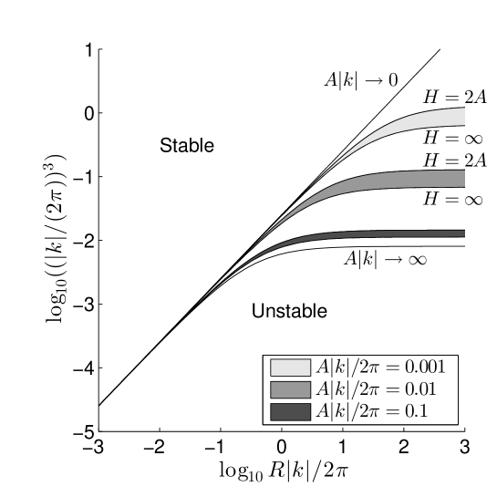
Figure 9: Plots of stability boundaries for sinusoidal perturbations of infinite straight flags, in the space of dimensionless wavenumber and body inertia. Results are shown for three ratios of near-wall-distance to perturbation wavelength ($A|k|/2\pi$). For each value of $A|k|/2\pi$, a range of stability boundaries is obtained for $2\leq H/A<\infty$, shown by a shaded region.

These parameters are used because $|k|^{3}$ scales with bending rigidity $B$ in the same way as $R_{2}$, and $R|k|$ scales with flag and fluid density in the same way as $R_{1}$. This can be seen by denoting the dimensional wavenumber by $\bar{k}$ and dimensional wavelength by $\lambda=2\pi/|\bar{k}|$, so that

$$\frac{R|k|}{2\pi}=\frac{RL|\bar{k}|}{2\pi}=\frac{\rho_{s}h}{\rho_{f}\lambda}\;;\;\left(\frac{|k|}{2\pi}\right)^{3}=\left(\frac{|\bar{k}|L}{2\pi}\right)^{3}=\frac{B}{\rho_{f}U^{2}W\lambda^{3}}$$ (25)

These parameters are equivalent to $R_{1}$ and $R_{2}$ when the finite flag length is replaced with the wavelength of the perturbation of the infinite flag.

In figure 9 we plot stability boundaries in the space of $R|k|/2\pi$ and $(|k|/(2\pi))^{3}$, for different dimensionless channel spacings, given by the near-wall-spacing $A|k|/2\pi=A/\lambda$ and the channel width ratio $H/A$. The lowest line, labeled $A|k|\to\infty$, is for an unbounded flow, and agrees with previous results Shelley, Vandenberghe, and Zhang (2005); Alben and Shelley (2008). Above the line, the flat state is stable, and below the line it is unstable. Above this line are the stability boundaries for channel-bounded flows. The shaded regions are a continuous range of stability boundaries for a given value of $A|k|/2\pi$ (labeled in the figure legend) and the full range of possible $H/A$ from 2 to $\infty$. As $A|k|/2\pi$ decreases, the shaded regions move upward, meaning the flag becomes less stable, as was found for the finite flag. And as $H/A$ decreases from $\infty$ down to 2, the stability boundary moves upward through each shaded region. Both results can be summarized with the statement that for “heavier” flags ($R|k|/2\pi\gtrsim 1$), the narrower the channel, the less stable the flag, in agreement with the finite flag. As $R|k|/2\pi$ decreases, all the stability boundaries converge. For the finite flag, the stability boundaries in Fig. 3 are quite close at small $R_{1}$ (the analog of $R|k|/2\pi$), but there is a slight variation that correlates with the channel spacing.

When $A|k|\to\infty$, the stability boundary is similar to those for the unbounded finite flag in Fig. 3, agreeing quantitatively at smaller inertia (if ($R_{1},R_{2}$) is identified with ($R|k|/2\pi$,$|k|^{3}/(2\pi)^{3}$)) and also reaching a plateau at larger inertia, though the values at which the plateaus occur in $R_{2}$ and $|k|^{3}/(2\pi)^{3}$ differ by about one decade. Apparently the presence of the wake is less important with smaller-wavelength perturbations. This was found previously for the unbounded flagAlben and Shelley (2008) and for flapping foilsAlben (2008b) .

V Conclusion

In this work we have investigated some of the basic effects of channel confinement on the flag flutter instability and large-amplitude flapping dynamics. For the infinite flag, we found a closed-form expression for the stability boundaries. In general, greater confinement increases the size of the instability region, although the effect mainly occurs with heavier bodies, and disappears for lighter bodies. For the finite flag, channel confinement has a similar effect on the stability boundary location. We found that multiple large-amplitude flapping states are possible but rare at parameters where periodic dynamics are found. We quantified the large-amplitude dynamics with three quantities: the flapping amplitude, the dominant frequency, and the time-averaged number of extrema in the flag’s deflection (analogous to the wavenumber). We studied the behavior of these quantities as the near-wall distance decreases, for symmetric and asymmetric channels. Starting from its unbounded value, the amplitude increases slightly as the channel walls approach in a symmetric channel, then decreases roughly in proportion to the channel wall spacing. The amplitude may be extremely close to the near-wall distance ($<$ 0.1 % in relative magnitude), or much smaller (20-50%), when the channel walls are much smaller than the flag length. Meanwhile, the frequency and number of extrema undergo a sequence of slight increases punctuated by large jumps. As the wall spacing decreases, the flag amplitude may decrease greatly with little change in the frequency and number of extrema. But at certain wall spacing values, the flag jumps to a higher flapping mode. The results are similar for an a very asymmetric channel, except that the flag flaps with a larger amplitude on the less bounded side.

An important future work is to compare these results with simulations of the fully viscous flow, to understand how the flag-wall interaction is modified by the presence of a viscous boundary layer.