Light Hadron Production in Proton-Proton Collisions at Different LHC Energies: Measured Data versus a Model

Abstract

Experiments involving proton-proton collisions at energies $\sqrt{s_{NN}}$ = 0.9, 2.76 and 7 TeV in Large Hadron Collider (LHC) have produced a vast amount of high-precision data. Here, in this work, we have chosen to analyse the two aspects of the measured data, viz., (i) the $p_{T}$ -spectra of pions, kaons, proton-antiproton at above-mentioned energies, and (ii) some of their very important ratio-behaviours, in the light of a version of the Sequential Chain Model (SCM). The agreements between the measured data and model-based results are generally found to be modestly satisfactory.

Keywords: Relativistic heavy ion collisions, baryon production, light mesons

PACS nos.: 25.75.-q, 13.60.Rj, 14.40.Be

The production of hadronic particles in high energy heavy ion physics is of special interest to understand the underlying mechanisms leading to such reaction products and to test the predictions from non-perturbative QCD processes. The yield of identified hadrons, their multiplicity distributions, the rapidity and transverse momentum spectra are the basic observables in heavy ion collisions. The measurement of such global observables has produced over the years, new and interesting insights about the involved production mechanisms, allowing in turn to improve the theoretical description of multiparticle production processes in heavy ion collisions.

In $pp$ collisions at ultra-relativistic energies $\sqrt{s_{NN}}$= 0.9, 2.76 and 7 TeV, the bulk of the particles produced at mid-rapidity have transverse momenta below 2 GeV/c. First principles calculations based on perturbative QCD are not able to provide detailed predictions of particle production.[1] Here, our basic objective in the present work is to interpret a part of significant data, like the transverse momenta spectra and some ratio-behaviours of pions, kaons and protons, obtained from $pp$ collisions at LHC energies $\sqrt{s_{NN}}$= 0.9, 2.76 and 7 TeV, with the help of the Sequential Chain Model (SCM). The another goal of the present work is to put this alternative approach to a segment of LHC-data with a view to assessing the success(es)/failure(s) of it.

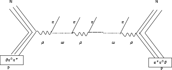
Figure 1: Feynman diagrams for the production of $\pi$ in the Sequential Chain Model

According to this Sequential Chain Model (SCM), high energy hadronic interactions boil down, essentially, to the pion-pion interactions; as the protons are conceived in this model as $p$ = ($\pi^{+}$$\pi^{0}$$\vartheta$) where $\vartheta$ is a spectator particle needed for the dynamical generation of quantum numbers of the nucleons [2]-[6]. The production of pions in the present scheme occurs as follows: the incident energetic $\pi$-mesons in the structure of the projectile proton(nucleon) emits a rho($\varrho$)-meson in the interacting field of the pion lying in the structure of the target proton, the $\varrho$-meson then emits a $\pi$-meson and is changed into an omega($\omega$)-meson, the $\omega$-meson then again emits a $\pi$-meson and is transformed once again into a $\varrho$-meson and thus the process of production of pion-secondaries continue in the sequential chain of $\varrho$-$\omega$-$\pi$ mesons. The production mechanism is shown schematically in Fig. 1. The two ends of the diagram contain the baryons exclusively [2]-[6].

In a similar fashion, the $K^{-}$($K^{+}$) and the baryon-antibaryon have been produced in the SCM and they are shown in Fig.2 and Fig.3 respectively.

The fundamental expressions for final (analytical) calculations are derived here on the basis of field-theoretic considerations and the use of Feynman diagram techniques with the infinite momentum frame tools and under impulse approximation method. The expressions for inclusive cross-sections of the $\pi^{-}$, $K^{-}$ and $\bar{p}$-secondaries would pick up from [2]-[6] and they are given by the following relations;

$$E\frac{d^{3}\sigma}{dp^{3}}|_{pp\rightarrow\pi^{-}x}\cong\Gamma_{\pi^{-}}\exp(-2.38<n_{\pi^{-}}>_{pp}x)\frac{1}{p_{T}^{(N_{R}^{\pi^{-}})}}\exp(\frac{-2.68p_{T}^{2}}{<n_{\pi^{-}}>_{pp}(1-x)})~{},$$ (1)

with

$${<n_{\pi^{+}}>_{pp}~{}\cong~{}<n_{\pi^{-}}>_{pp}~{}\cong~{}<n_{\pi^{0}}>_{pp}~{}\cong~{}1.1s^{1/5}~{},}$$ (2)

$$E\frac{d^{3}\sigma}{dp^{3}}|_{pp\rightarrow K^{-}x}~{}\cong~{}\Gamma_{K^{-}}\exp(-6.55<n_{K^{-}}>_{pp}x)~{}\frac{1}{p_{T}^{(N_{R}^{K^{-}})}}\exp(\frac{-1.33p_{T}^{2}}{<n_{K^{-}}>^{3/2}_{pp}})~{}~{},$$ (3)

and with

$$<n_{K^{+}}>_{pp}\cong<n_{K^{-}}>_{pp}\cong<n_{K^{0}}>_{pp}\cong<n_{\bar{K^{0}}}>_{pp}\cong 5\times 10^{-2}s^{1/4},$$ (4)

$$E\frac{d^{3}\sigma}{dp^{3}}|_{pp\rightarrow{\bar{p}}x}~{}\cong\Gamma_{\bar{p}}\exp(-25.4<n_{\bar{p}}>_{pp}x)\frac{1}{p_{T}^{({N_{R}}^{\bar{p}})}}\exp(\frac{-0.66((p_{T}^{2})_{\bar{p}}+{m_{\bar{p}}}^{2})}{<n_{\bar{p}}>^{3/2}_{pp}(1-x)})~{},$$ (5)

with $m_{\bar{p}}$ is the mass of the antiprotons. For ultrahigh energies

$${<n_{\bar{p}}>_{pp}~{}\cong<n_{p}>_{pp}~{}\cong~{}2\times 10^{-2}~{}s^{1/4}~{}.}$$ (6)

where $\Gamma_{C^{-}}$ ($C^{-}$ stands for $\pi^{-}$, $K^{-}$ or $\bar{p}$) is the normalisation factor which will increase as the inelastic cross-section increases and it is different for different energy region and for various collisions. The terms $p_{T}$, $x$ in equations (1), (3) and (5) represent the transverse momentum, Feynman Scaling variable respectively. Moreover, by definition, $x~{}=~{}2p_{L}/{\sqrt{s}}$, where $p_{L}$ is the longitudinal momentum of the particle. The $s$ in equations (2), (4) and (6) is the square of the c.m. energy.

$1/p_{T}^{N_{R}^{C^{-}}}$ represnts the ‘constituent rearrangement term’ arising out of the partons inside the proton which essentially provides a damping term in terms of a power-law in $p_{T}$ with an exponent of varying values depending on both the collision process and the specific $p_{T}$-range. The choice of ${N_{R}}$ would depend on the following factors: (i) the specificities of the interacting projectile and target, (ii) the particularities of the secondaries emitted from a specific hadronic or nuclear interaction and (iii) the magnitudes of the momentum transfers and of a phase factor (with a maximum value of unity) in the rearrangement process in any collision. And this is a factor for which we shall have to parameterize alongwith some physics-based points indicated earlier. The parametrization is to be done for two physical points, viz., the amount of momentum transfer and the contributions from a phase factor arising out of the rearrangement of the constituent partons. Collecting and combining all these, the relation is to be given by [7]

$$N_{R}=4<N_{part}>^{1/3}\theta,$$ (7)

where $<N_{part}>$ denotes the average number of participating nucleons and $\theta$ values are to be obtained phenomenologically from the fits to the data-points.

On the average, the particles are produced in charge-independent equal measure, for which roughly one-third of the particles could be reckoned to be positively charged, one third are negatively charged and the rest one third are neutral. But, according to the present mechanism of particle production, there are some specifically exclusive means to produce positive particles, of which $\pi^{+}$, $K^{+}$, and $p$ are the members. They are produced from within the structure of protons (nucleons). These production characteristics and the quantitative expressions for their special production have been dwelt upon in detail in Ref. [6]. Let us assort the relevant expressions therefrom as results to be used here.

For production of positive pions [$\pi^{+}$ mesons] the excess term could be laid down by the following expressions [6]:

$$(B_{\pi^{+}})_{pp}={\frac{4}{3}}{g^{2}_{p\pi\pi}}{\frac{(P^{\prime}+K)^{2}}{[(P^{\prime}+K)^{2}-m_{p}^{2}]^{2}}}A(\nu,q^{2})_{\pi}\int{\frac{d^{3}k_{\pi}}{2k_{0}(2\pi)^{3}}\exp(-ik_{\pi}x)},$$ (8)

where the symbols have their contextual connotation with the following hints to the physical reality of extraneous $\pi^{+}$, as non-leading secondaries. The first parts of the above equations (Eqn.(8)), contain the coupling strength parameters, the second terms of the above equations are just the propagator for excited nucleons. The third terms represent the common multiparticle production amplitudes along with extraneous production modes and the last terms indicate simply the phase space integration terms on the probability of generation of a single $\pi^{+}$. These expressions are to be calculated by the typical field-theoretical techniques and are to be expressed – if and when necessary – in terms of the relevant variable and/or measured observables.

In order to arrive at the transverse momentum distribution of $\pi^{+}$, one has to consider the Eqn. (1), along with eqn. (8). For excess $\pi^{+}$ production, a factor represented by $(1+\gamma^{\pi^{+}}p_{T}^{\pi^{+}})$ is to be operated on inclusive cross-section as an multiplier [6].

Adopting the above procedure, as we indicated for the production of positive pions, we obtain for the transverse momentum distribution of $K^{+}$ a multiplicative factor $\sim(1+\gamma^{K^{+}}p_{T}^{K^{+}})$ to be operated on the inclusive cross-section of $K^{-}$ production. [6].

Similarly, for the production of protons, we obtain for the transverse momentum distribution of $p$ by operating a multiplicative factor $\sim(1+\gamma^{p}p_{T}^{p})$, on inclusive cross-section of $\bar{p}$.

We will dwell upon here properties of the nature of $p_{T}$-spectra and some particle-production ratios of some light hadrons, like $\pi^{\pm}$, $K^{\pm}$, $\bar{p}$ and $p$, in $pp$-collisions at energies $\sqrt{s_{NN}}$= 0.9, 2.76 and 7 TeV in LHC.

The general form of our SCM-based transverse-momentum distributions for $p+p\rightarrow C^{-}+X$-type reactions can be written in the following notation:

$${\frac{1}{2\pi p_{T}}\frac{d^{2}N_{C}}{d\eta dp_{T}}|_{p+p\rightarrow C^{-}+X}=\alpha_{C^{-}}\frac{1}{p_{T}^{N_{R}^{C^{-}}}}\exp(-\beta_{C^{-}}\times p_{T}^{2}).}$$ (9)

The values of $\alpha_{\pi^{-}}$ and $\beta_{\pi^{-}}$ , for example, can be calculated from the following relations [equation 1]:

$${\alpha_{\pi^{-}}=\Gamma_{\pi^{-}}\exp(-2.38<n_{\pi^{-}}>_{pp}x)}$$ (10)

$${\beta_{\pi^{-}}=\exp(\frac{-2.68}{<n_{\pi^{-}}>_{pp}(1-x)})}$$ (11)

And for calculation of $(N_{R}^{\pi^{-}})_{pp}$, we use eqn.(7). The values of $(\alpha_{C^{-}})_{pp}$, $(N_{R}^{C^{-}})_{pp}$ and $(\beta_{C^{-}})_{pp}$ for $K^{-}$ and $\bar{p}$ can be calculated in a similar way by using equations (3)-(6).

The values of $(\alpha_{C^{-}})_{pp}$, $(N_{R}^{C^{-}})_{pp}$ and $(\beta_{C^{-}})_{pp}$ ($C^{-}$ stands for $\pi^{-}$, $K^{-}$ or $\bar{p}$ respectively.) for different energies are given in the left panels of Table 1. The experimental data for the inclusive cross-sections versus $p_{T}$ [GeV/c] for $\pi^{-}$, $K^{-}$ and $\bar{p}$ production in $p+p$ interactions at $\sqrt{s_{NN}}$ = 0.9, 2.76 and 7 TeV are taken from Ref. [8] and they are plotted in Figs. 4(a), 4(c) and 4(e) respectively. The solid lines in those figures depict the SCM-based plots while the dotted lines show the Pythia-induced calculations.

In order to arrive at the transverse momentum distribution of $\pi^{+}$, $K^{+}$ and $p$ one has to consider the Eqn. (1), eqn. (4), eqn. (6), eqn. (8), eqn. (9) along with eqn. (10). For excess $\pi^{+}$ production, the factor $(1+\gamma^{\pi^{+}}p_{T}^{\pi^{+}})$ is to be operated on $\frac{1}{2\pi p_{T}}\frac{d^{2}N}{dp_{T}dy}|_{p+p\rightarrow\pi^{-}+X}$ as an multiplier. $\gamma^{\pi^{+}}\simeq(20\pi g^{2}_{{\rho}{\pi}{\pi}}/<n_{\pi}>)/\sqrt{s}\simeq 0.44$ [3]. Taking $<p_{T}>_{\pi^{+}}\simeq 0.31$ GeV/c [9], the calculated values of $\alpha_{\pi^{+}}$ for different energies are given in the right panel of Table 1. The values of $(N_{R}^{\pi^{+}})_{pp}$ and $(\beta_{\pi^{+}})_{pp}$ are remain same and they are given in the right panel of Table 1.

Similarly, we obtain for the transverse momentum distribution of $K^{+}$, the multiplicative factor $\sim(1+\gamma^{K^{+}}p_{T}^{K^{+}})$ is to be operated on $\frac{1}{2\pi p_{T}}\frac{d^{2}N}{dp_{T}dy}|_{p+p\rightarrow K^{-}+X}$ as an multiplier.The $\gamma^{K^{+}}$ has been calculated $\gamma^{K^{+}}\simeq(4\pi g^{2}_{KN\Lambda}+4\pi g^{2}_{\Sigma KN})/2\sqrt{s}\simeq 0.082$ [3]. We use the value of $<p_{T}>_{K^{+}}\simeq 0.36$ GeV/c [9]. The right panel of Table 1 depicts all calculated values of $\alpha_{K^{+}}$, $N_{R}^{K^{+}}$ and $\beta_{K^{+}}$.

And we obtain for the transverse momentum distribution of $p$ by operating a multiplicative factor $\sim(1+\gamma^{p}p_{T}^{p})$ on $\frac{1}{2\pi p_{T}}\frac{d^{2}N}{dp_{T}dy}$. The value of $\gamma^{p}\sim 0.32$ [3] and by taking $<p_{T}>_{p}\simeq 0.50$ GeV/c [9]. The right panel of Table 1 depicts all calculated values of $\alpha_{p}$, $N_{R}^{p}$ and $\beta_{p}$ for energies $\sqrt{s_{NN}}$ = 0.9, 2.76 and 7 TeV. In Figures 4(b), 4(d) and 4(f), we have plotted experimental versus theoretical results for $\pi^{+}$ , $K^{+}$ and $p$ production in $p+p$ collisions at energies $\sqrt{s_{NN}}$ = 0.9, 2.76 and 7 TeV, respectively. Data are taken from the Refs. [8]. The solid lines in those Figures are the SCM-based plots while the dotted lines show the PYTHIA-induced calculations.

The $(K^{+}+K^{-})/(\pi^{+}+\pi^{-})$ and $(p+\bar{p})/(\pi^{+}+\pi^{-})$ ratios at energies $\sqrt{s_{NN}}$ = 0.9, 2.76 and 7 TeV have been calculated from eqn. (9) and Table 1 and the results are plotted in Figs. 5(a), 5(c) and 5(e). Data are taken from the Refs. [8] and [10]. Similarly, $\pi^{-}/\pi^{+}$, $K^{-}/K^{+}$ and $\bar{p}/p$-ratios are plotted in the right panel of Fig. (5), i.e., Figs. 5(b), 5(d) and 5(f). Data are taken from the Refs. [8]. The solid lines in those Figures are the average SCM-based plots.

Let us make some general observations and specific comments on a case-to-case basis.

1) The very basic model used here is essentially of non-standard type. The measures of invariant yields against transverse momenta ($p_{T}$) obtained on the basis of the SCM for pions, kaons and protons at LHC energies $\sqrt{s_{NN}}$= 0.9, 2.76 and 7 TeV are depicted in Fig. (4). The calculated values of $(\alpha_{C})_{pp}$, $(N_{R}^{C})_{pp}$ and $(\beta_{C})_{pp}$ ($C$ stands for $\pi$, $K$ or $p$ respectively.) of eqn.(9) have been shown in Table 1. Besides, we compare the model-based calculations with the PYTHIA-based results. Comparisons show neither sharp disagreement nor any good agreement between these two. Results show a modest degree of success.

There are some disagreements of the model in describing the data in the low-$p_{T}$ region. These are due to the fact that the model has turned essentially into a mixed one with the inclusion of power law due to the inclusion of partonic rearrangement factor. This power law term disturbs, to a considerable extent, the agreement between the data and the model. However, the power-law part of the equation might not be the only factor for this type of discrepancy. The initial condition and dynamical evolution in heavy-ion collisions are more complicated than we expect. Till now, we do not know the exact nature of reaction mechanism. One might take into account some other factors like radial flow or thermal equilibrium. The thermal equilibrium was included in blast-wave model in a recent paper. [11] But we are not able to include these factors. The model is, thus, different from thermal model and blast-wave model [11] in some way. These are the factors that the model is lagging.

2) The calculated values of $K/\pi$ and $p/\pi$ are compared with the experimental ones and they are plotted in Figs. 5(a), 5(c) and 5(e). The $K/\pi$ ratios show a modest degree of success while for $p/\pi$, the theoretical values differ slightly from the experimental ones in the low-$p_{T}$ part. In a similar way, $\pi^{-}/\pi^{+}$, $K^{-}/K^{+}$ and $\bar{p}/p$-ratios are plotted in the right panel of Fig. (5). Here, the model reproduce the data modestly well.

One point needs to be addressed here. The $K^{-}/K^{+}$-ratios at $\sqrt{s_{NN}}$= 0.9, 2.76 and 7 TeV are calculated from Table 1 and they are $\sim$ 0.98, 0.98 and 0.98 respectively. This is due to extraneous mode of production of positive particles. No hyperon has been produced in the present scheme of the SCM. The production mechanism of kaons are shown schematically in Fig. 2.

However, on the overall basis, the total approach might provide an alternative route to understand and interpret the behaviour of high energy collisions.
Acknowledgements
The authors are very much thankful to the learned Referees for their valued comments and constructive criticisms.

Table 1: Values of $\alpha$, $N_{R}$ and $\beta$ for pions, kaons, antiproton and proton productions in $p+p$ collisions at $\sqrt{s_{NN}}$=0.9, 2.76 and 7 TeV

$\pi^{-}$ $\pi^{+}$

$\sqrt{s_{NN}}$=0.9 TeV

$\alpha_{\pi^{-}}$ $N_{R}^{\pi^{-}}$ $\beta_{\pi^{-}}$ $\alpha_{\pi^{+}}$ $N_{R}^{\pi^{+}}$  $\beta_{\pi^{+}}$

0.310 2.054 0.128 0.350 2.054 0.128

$\sqrt{s_{NN}}$=2.76 TeV

$\alpha_{\pi^{-}}$ $N_{R}^{\pi^{-}}$ $\beta_{\pi^{-}}$ $\alpha_{\pi^{+}}$ $N_{R}^{\pi^{+}}$ $\beta_{\pi^{+}}$

0.461 2.163 0.085 0.521 2.163 0.085

$\sqrt{s_{NN}}$=7 TeV

$\alpha_{\pi^{-}}$ $N_{R}^{\pi^{-}}$ $\beta_{\pi^{-}}$ $\alpha_{\pi^{+}}$ $N_{R}^{\pi^{+}}$ $\beta_{\pi^{+}}$

0.602 2.183 0.075 0.683 2.183 0.075

$K^{-}$ $K^{+}$

$\sqrt{s_{NN}}$=0.9 TeV

$\alpha_{K^{-}}$ $N_{R}^{K^{-}}$ $\beta_{K^{-}}$ $\alpha_{K^{+}}$ $N_{R}^{K^{+}}$ $\beta_{K^{+}}$

0.130 1.354 0.248 0.133 1.354 0.248

$\sqrt{s_{NN}}$=2.76 TeV

$\alpha_{K^{-}}$ $N_{R}^{K^{-}}$ $\beta_{K^{-}}$ $\alpha_{K^{+}}$ $N_{R}^{K^{+}}$ $\beta_{K^{+}}$

0.145 1.414 0.148 0.147 1.414 0.148

$\sqrt{s_{NN}}$=7 TeV

$\alpha_{K^{-}}$ $N_{R}^{K^{-}}$ $\beta_{K^{-}}$ $\alpha_{K^{+}}$ $N_{R}^{K^{+}}$ $\beta_{K^{+}}$

0.195 1.454 0.134 0.198 1.454 0.134

$\bar{p}$ $p$

$\sqrt{s_{NN}}$=0.9 TeV

$\alpha_{\bar{p}}$ $N_{R}^{\bar{p}}$ $\beta_{\bar{p}}$ $\alpha_{p}$ $N_{R}^{p}$ $\beta_{p}$

0.073 1.154 0.248 0.085 1.154 0.248

$\sqrt{s_{NN}}$=2.76 TeV

$\alpha_{\bar{p}}$ $N_{R}^{\bar{p}}$ $\beta_{\bar{p}}$ $\alpha_{p}$ $N_{R}^{p}$ $\beta_{p}$

0.095 1.243 0.148 0.108 1.243 0.148

$\sqrt{s_{NN}}$=7 TeV

$\alpha_{\bar{p}}$ $N_{R}^{\bar{p}}$ $\beta_{\bar{p}}$ $\alpha_{p}$ $N_{R}^{p}$ $\beta_{p}$

0.120 1.263 0.134 0.130 1.263 0.134

Figure 2: Feynman diagrams for the production of $K^{\pm}$ in the Sequential Chain Model

Figure 3: Feynman diagrams for the production of $\bar{p}$ and $p$ in the Sequential Chain Model.

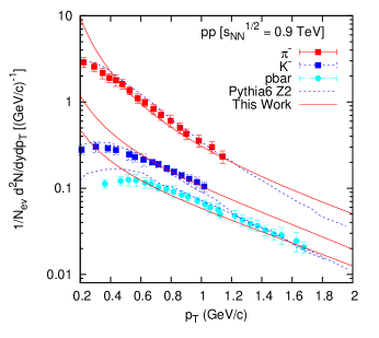
2.6in

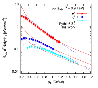
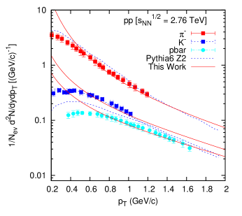
2.6in

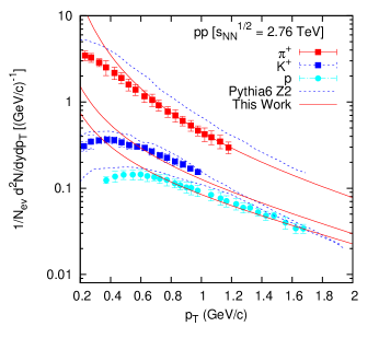
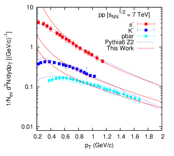
2.6in

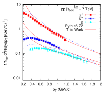
Figure 4: Plots for $\pi$, $K$, $\bar{p}$ and $p$ productions in $p+p$ collisions at energies $\sqrt{s_{NN}}$ = 0.9 TeV, $\sqrt{s_{NN}}$ = 2.76 TeV and $\sqrt{s_{NN}}$ = 7 TeV. Data are taken [8]. Solid lines in the Figures show the SCM-based theoretical plots while the dotted ones show PYTHIA-based results [8].

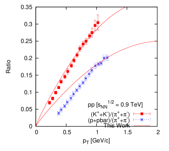
2.6in

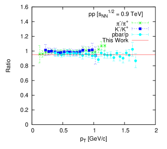
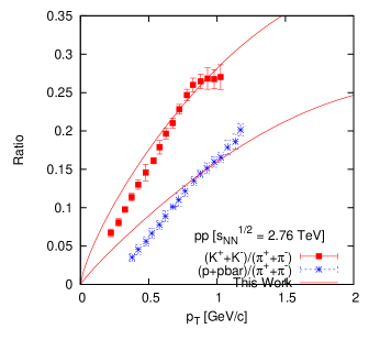
2.6in

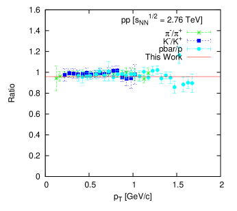
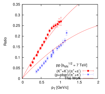
2.6in

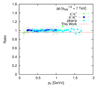
Figure 5: Ratio behaviours for different hadrons at different LHC-energies. The figures in the left panel depict $K/\pi$ and $p/\pi$ ratios whereas the right panel shows $\pi^{-}/\pi^{+}$, $K^{-}/K^{+}$ and $p/{\bar{p}}$ ratio behaviour at energies $\sqrt{s_{NN}}$ = 0.9 TeV, $\sqrt{s_{NN}}$ = 2.76 TeV and $\sqrt{s_{NN}}$ = 7 TeV. Data are taken from [8], [10]. Lines in the Figures show the SCM-based theoretical plots.

References

- [1] Riggi F 2013 Journal of Physics: Conference Series 424, 012004
- [2] Guptaroy P, Sau G, Biswas S K Bhattacharyya S 2010 IL Nuovo Cimento B 125, 1071
- [3] Guptaroy P, De B, Sau G, Biswas S K Bhattacharyya S 2007 Int. J. Mod. Phys. A 28,5121 and the references therein
- [4] Bandyopadhyay P and Bhattacharyya S 1978 IL Nuovo Cimento A 43, 305
- [5] Bhattacharyya S 1988 IL Nuovo Cimento C 11, 51
- [6] Bhattacharyya S 1988 J. Phys. G 14, 9
- [7] Guptaroy P, Sau G, Biswas S K Bhattacharyya S 2008 Mod. Phys. Lett. A 23, 1031
- [8] Chatrchyan S et al, CMS Collaboration 2012 Eur. Phys. J. C 72, 2164
- [9] Alver B et al 2008 Phys. Rev. C 77, 061901
- [10] Preghenella R (for the ALICE Collaboration) 30 Nov 2011 arXiv:1111.7080v1 [hep-ex]
- [11] Zhang S, Han L X, Ma Y G, Chen J H and Zhong C 2014 Phys. Rev C 89, 034918