Anderson’s considerations on the flow of superfluid helium:
some offshoots

Abstract

Nearly five decades have elapsed since the seminal 1966 paper of P.W. Anderson on the flow of superfluid helium, ⁴He at that time. Some of his “Considerations” – the role of the quantum phase as a dynamical variable, the interplay between the motion of quantised vortices and potential superflow, its incidence on dissipation in the superfluid and the appearance of critical velocities, the quest for the hydrodynamic analogues of the Josephson effects in helium – and the way they have evolved over the past half-century are recounted below. But it is due to key advances on the experimental front that phase slippage could be harnessed in the laboratory, leading to a deeper understanding of superflow, vortex nucleation, the various intrinsic and extrinsic dissipation mechanisms in superfluids, macroscopic quantum effects and the superfluid analogue of both ac and dc Josephson effects – pivotal concepts in superfluid physics – have been performed. Some of the experiments that have shed light on the more intimate effect of quantum mechanics on the hydrodynamics of the dense heliums are surveyed, including the nucleation of quantised vortices both by Arrhenius processes and by macroscopic quantum tunnelling, the setting up of vortex mills, and superfluid interferometry.

Superfluids display quantum properties over large distance. Superfluid currents may persist indefinitely unlike those of ordinary fluids (Reppy and Lane, 1965); the circulation of flow velocity has been found quantised over meter-size paths (Verbeek et al., 1974). These manifestations of macroscopic quantum phenomena have constituted one of the early hallmarks of experimental condensed matter physics as reviewed over the years by a number of authors. They are viewed as supporting the concept of a macroscopic wavefunction extending over the whole superfluid sample as put forward by London (1954). Together with Landau’s views on the irrotational nature of superfluid motion Landau (1941), these ideas form the basis of the two-fluid model, summarised in Sec.I, which not only describes the hydrodynamics of superfluids (Khalatnikov, 1965) but has been extended to other fields of physics like superconductivity, the Bose-Einstein condensed gases$\ldots$ (Enz, 1974)

Hydrodynamics, and superfluid hydrodynamics in its wake, is expected to break down at small scale when the typical lengths of the problem at hand are no longer much larger than the interatomic separation or other microscopic lengths characteristic of the internal structure of the fluid, the “size” of Cooper pairs in superfluid ³He for instance. It has however been known for a long time, notably from the ion propagation measurements of Rayfield and Reif (1964) that the relevant scale in superfluid ⁴He is surprisingly small, of the order of ångströms. In these experiments, the velocity of vortex rings could be measured in a direct way and compared to the usual outcome of classical hydrodynamics (see Sec.II). Rayfield and Reif found that, at first sight at least, hydrodynamics remains valid down to atomic sizes. Their result holds for ⁴He, which is a dense fluid of bosons. The relevant scale is much larger in superfluid ³He, a BCS-type p-wave superfluid in which the characteristic length is fixed by the “size” of the Cooper pair. This article aims at reviewing how the hydrodynamics of superfluid ⁴He and ³He evolves from large to small scale and ultimately breaks down at close distance, revealing the more intimate quantum properties of these fluids. This is no mean feat, as noted long ago by Uhlenbeck, who is quoted to have said “One must watch like a hawk to see Planck’s constant appear in hydrodynamics” Putterman (1974).

The main object of study in the following is the time and space evolution of the phase of the macroscopic wavefunction, often simply referred to as “the phase”, in so-called aperture flow. This concept of “phase” with wave-mechanical properties governing the evolution of macroscopic quantities has become so well-spread that its meaning is, wrongly perhaps, taken for granted. It was put forward by P. W. Anderson in 1966, following the lead of Feynman (1955), mainly by the recognition of the phase as the quantity commandeering in superfluids both the putative Josephson-type effects and dissipation caused by vortex motion. The dynamics of quantised vortices, central to Anderson’s ideas, is outlined in Sec.II. A detailed understanding of these phenomena is of fundamental importance as they govern the breakdown of viscousless flow – the most noteworthy feature of superfluidity – and the appearance of an entirely new class of phenomena – the hydrodynamic analogues of the Josephson effects – that underpin the sort of interferometry that can be performed with the superfluid wavefunction.

These ideas were agitated in the mid-sixties, in particular at the Sussex Meeting in 1965, by Anderson (1966a), and by a number of prominent physicists, notably Nozières and Vinen. Reliable experimental observations were performed twenty years later only, as recalled in Sec.III, giving a host of new results and insights on superfluid hydrodynamics, notably an improved understanding of critical velocities and of the nucleation of vortices, topics discussed in Secs.IV and V, of possible mechanisms for formation of vortex tangles, described in Sec.VI, of the appearance of the Josephson regime of superflow through tiny apertures, described in Sec.VII.

Presented below is a coverage of some of the ramifications of Anderson’s ideas on phase slippage in superfluids. It is intended to provide a gangway between the many excellent monographs that provide the background material on this subject and the more specialised research publications in the literature that give the full, raw, sometimes arcane, coverage. As such, it does not constitute a comprehensive review - space and time constraining - but touches on a few selected issues that provide the backbone of this subfield of superfluid hydrodynamics. Reviews with different flavours span over a quarter of a century and show how this field has evolved.

Particularly worthy of notice are the reviews of closely related subjects, Sonin’s description of vortex dynamics ((Sonin, 1987, 2015), the Landau critical velocity in superfluid ⁴He by McClintock and Bowley (1995) and in superfluid ³He-B by Dobbs (2000), and vortex formation and dynamics in superfluid ³He by Eltsov et al. (2005); Salomaa and Volovik (1987); Volovik (2003). The later references also cover the exciting field of exotic topological defects in superfluid ³He under rotation, not considered here.

I The basic superfluid: He-4

Helium-4 undergoes an ordering transition toward a superfluid state at $T\sim 2.17$ K under its saturated vapour pressure (SVP), which is now commonly viewed as a form of Bose-Einstein condensation. A similar transition occurs in helium-3 at $T\lesssim 2.7$ mK when Cooper pairing in a state with parallel spin $S=1$ and relative orbital momentum $l=1$ occurs.

I.1 The two-fluid hydrodynamics

The flowing superfluid helium must obey some form of hydrodynamic equations given by the general conservation laws, Galilean invariance, and the thermodynamic equation of state that should also include its superfluid properties. These equations were written down for ⁴He by Landau (1941) (Landau and Lifshitz, 1959; Khalatnikov, 1965) who made the key assumption that in order to describe the viscous-less fluid flow the independent hydrodynamical variables must include a velocity field $\mathbf{v}_{\mathrm{s}}$, to which is associated a fraction $\rho_{\mathrm{s}}/\rho$ of the total density of the liquid, $\rho=m_{4}/v_{4}$ being the ⁴He atomic mass divided by the volume occupied by one atom. This ideal inviscid fluid velocity field conforms to the Euler equation for ideal fluid flow. As a consequence, it also obeys the Kelvin-Helmholtz theorem, which states that the vorticity $\nabla\times\mathbf{v}_{\mathrm{s}}$ remains constant along the fluid flowlines. In addition to vorticity conservation, a more stringent condition was assumed by Landau (1941), namely that the superfluid velocity field be at any instant irrotational at all points in the superfluid:

$$\nabla\times\mathbf{v}_{\mathrm{s}}=0\;.$$ (1)

The superfluid fraction velocity therefore derives from a velocity potential. This property will be shown below to be intimately related to the microscopic description of the superfluid and to have far-reaching consequences.

The remainder of the fluid, the normal fraction $\rho_{\mathrm{n}}=\rho-\rho_{\mathrm{s}}$, to which is associated a “normal” velocity $\mathbf{v}_{\mathrm{n}}$, obeys an equation similar to the Navier-Stokes equation of viscous flow. The total momentum density of the helium liquid is the sum of the contributions of these two fluids:

$$\mathbf{j}=\rho_{\mathrm{s}}\mathbf{v}_{\mathrm{s}}+\rho_{\mathrm{n}}\mathbf{v}_{\mathrm{n}}\;.$$ (2)

The superfluid part of the flow being assumed ideal, it carries no entropy. The fluid entropy is transported by the normal fluid described by Landau as a gas of thermally-excited elementary excitations, the phonons – or sound quanta – at long wavelengths and the rotons at wavelengths of the order of interatomic spacing, as sketched in Fig.1.

Figure 1: Dispersion curve of the elementary excitations in superfluid ⁴He as devised by Landau (1947).

Landau attributed the non-viscous property of ⁴He flow to the intrinsic shape of this spectrum. There exists no elementary excitation with a finite momentum $\bf p=\hbar\,\bf k$ and a small enough energy $\epsilon(\bf p)$ to couple to a solid obstacle or a wall at rest while conserving energy and momentum. At least for small enough superflow velocities. This requirement sets the Landau criterion for dissipationless flow: $v_{\mathrm{s}}<v_{\mathrm{L}}$. The intricate problem of critical velocities above which dissipation arises in superfluid flow is dealt with in Sec.IV.

When $\rho_{\mathrm{n}}$ and $\rho_{\mathrm{s}}$ can be assumed incompressible – i.e., for small flow velocities, the separation between potential flow for $\mathbf{v}_{\mathrm{s}}$ and a Poiseuille flow for $\mathbf{v}_{\mathrm{n}}$ becomes exact. In this approximation, superflow is effectively decoupled from normal fluid motion. It has become customary to talk somewhat loosely of the motion of the superfluid as fully distinct from that of the normal fluid. This simplified view is adopted here but, occasionally, it fails (Idowu et al., 2000a, b).

Landau’s two-fluid hydrodynamics, based on early experiments on superfluids and preceded by the original suggestion of Tisza (1938), accounts remarkably well for a whole class of thermodynamical and hydrodynamical properties, notably for the existence of second sound and for the non-classical rotational inertia in Andronikashvili oscillating-disks experiments (Andronikashvili and Mamaladze, 1966). It features full internal consistency; it assumes that the motion of $\rho_{\mathrm{s}}$ is pure potential (irrotational) flow and carries no entropy, and it reaches the conclusion that, below $v_{\mathrm{L}}$, this motion is indeed fully inviscid. It has been universally adopted.

The two-fluid hydrodynamics has been extended to the superfluid phases of ³He. A number of new features appear owing to the anisotropy introduced by the Cooper pairing in a $l=1$ state of orbital momentum. Some of these features are discussed in Sect.VII.2, but the separation of the hydrodynamics between a superfluid component and a “normal” component still holds as well as the existence of a Landau critical velocity.

However, this model has a number of shortcomings pointed out, among others, by London (1954). In particular, for the purpose of this review, it does not discuss the roots of the irrotationality condition, Eq. (1), which are to be found in the existence of a complex scalar order parameter arising from the transition to a Bose-condensed state, as recognised at a very early stage of the study of superfluids by London (1938). It gives no clue as to when the hydrodynamics of the superfluid fails at close distance as any macroscopic approach to hydrodynamic is bound to. Namely, it provides no way of estimating the superfluid coherence length - or healing length of the macroscopic wavefunction. It also completely disregards the existence of quantised vorticity, which, as recognised by Feynman (1955) and Anderson (1965), is responsible for dissipation of the superfluid motion and for different, and more commonly met in practice, critical velocity mechanisms than that of $v_{\mathrm{L}}$.

As already noted, the Landau criterion for critical velocities rests on the fact that the elementary excitation energy spectrum is sharply defined, that is, it rises linearly as $\epsilon=\mathrm{c}p$ with no spread in energy: there are no excitations with low energy and small moment capable of exchanging momentum with the superfluid in slow motion, thus causing dissipation. This sharpness of the energy spectrum $\epsilon(p)$ has been checked directly by neutron scattering measurements of the dynamic structure factor as discussed in particular by Glyde (1993, 2013).

It may be pointed out here that ³He in the normal Fermi liquid state does display an elementary excitation spectrum with a phonon branch and a roton minimum in neutron diffraction experiments (Stirling et al., 1976; Griffin, 1987). However, that spectrum is broad; ³He does not exhibit superfluid properties until Cooper pairs of fermions form and Bose-condense. As stressed by Feynman (1972), it really is the lack – the “scarcity” in Feynman’s words – of low-lying energy levels at finite momenta, a property of the $N$-boson groundstate with a macroscopic number of particles in it and the existence of few excited states well-separated in energy, that results in superfluidity.

I.2 The superfluid order parameter

A different approach to superfluidity in which a central role was attributed to the phase of the order parameter (assumed to describe this superfluidity) was sketchily framed by Onsager in 1948, as reported by London (1954). London himself did not make much use of this concept of phase, although, on the one hand, he was the first to propose that superfluidity arises from Bose-Einstein condensation and the appearance of a “macroscopic wave function”, and on the other hand, he had earlier realised the important significance of the phase factor in quantum mechanical wavefunctions.

Indeed, as soon as wavefunctions are considered, the concept of quantum phase becomes relevant. Its early origin can be found in a formalisation of electrodynamics by Weyl (Yang, 2003), in which a gauge transformation explicitly introduces a factor $\mathrm{e}^{\theta}$ in the theory. A change of gauge, $\mathbf{A}^{\prime}\longrightarrow\mathbf{A}+\nabla\theta$, combined with a change of the wavefunction $\psi^{\prime}\longrightarrow\psi\,\exp\{\mathrm{i}\,e\theta/\hbar c\}$ leaves the Schrödinger equation unchanged. The application of Weyl’s prescription to quantum-mechanical systems led F. London to turn the exponent $\theta$ into a purely imaginary quantity $\mathrm{i}\varphi$, $\varphi$ then having the significance of an actual phase (Yang, 2003). These historical developments explain the somewhat inadequate terminology that refers to changes of the phase as gauge transformations Greiter (2005).

But the unifying power of quantum field gauge theories ultimately carried the day. The fact that a droplet of superfluid randomly picks up a (well-defined) quantum phase when it nucleates out of vapour or out of normal fluid in a confined geometry, is referred to as the breaking of gauge symmetry. The term “Bose broken-symmetry” promoted in particular by Griffin (1987) to describe the appearance of a macroscopic number of particles in the groundstate of a Bose system with the same one-particle wavefunction exhibiting the same phase factor only gained limited acceptance.

The ground state wavefunction of a homogeneous system of structureless bosons such as superfluid ⁴He at rest can be shown quite generally to have no node; it reduces to a complex scalar with a constant phase and a modulus that remains finite at every point in the sample. Atomic motion results in small scale, small amplitude fluctuations of this complex scalar. Averaging these fluctuations over finite, but still small, volume elements leaves a “coarse-grained” average wavefunction. If the system is inhomogeneous on a scale much larger than the coarse-graining volume, the modulus and phase are slowly varying functions of the position $\mathbf{r}$,

$$\mathit{\Psi}(\mathbf{r})=f(\mathbf{r})\,\mathrm{e}^{\textstyle{\mathrm{i}\varphi(\mathbf{r})}}\;.$$ (3)

This in essence is the macroscopic wavefunction considered by London (1938), Onsager (1949), London (1954) and Feynman (1955, 1972). The information on the localisation of the bosons at $\mathbf{r}_{1},\mathbf{r}_{2},\ldots,\mathbf{r}_{\mathrm{N}}$ and on their short-range correlations has been lost in Eq.(3), which is not an exact many-body ground state wavefunction anymore. However, considered as a “macroscopic matter field” in Anderson’s own words, it has provided a lot of mileage in describing the properties of superfluids.

I.3 The superfluid velocity

The particle density $n(\mathbf{r})$ at point $\mathbf{r}$ of the $N$-boson system is given in terms of this macroscopic wavefunction, Eq.(3), by

$$n(\mathbf{r})=\int\mathrm{d}^{3}\mathbf{r}_{1}\ldots\mathrm{d}^{3}\mathbf{r}_{\mathrm{N}}\,\mathit{\Psi}^{\star}(\mathbf{r})\mathit{\Psi}(\mathbf{r})\,\sum_{i=1}^{\mathrm{N}}\delta(\mathbf{r}-\mathbf{r}_{i})\;,$$ (4)

and the particle current density by

$$\begin{split}\mathbf{j}(\mathbf{r})&=\int\mathrm{d}^{3}\mathbf{r}_{1}\ldots\mathrm{d}^{3}\mathbf{r}_{\mathrm{N}}\\ &\sum_{i=1}^{\mathrm{N}}\frac{\hbar}{2\mathrm{i}m_{4}}\bigg{[}\mathit{\Psi}^{\star}(\mathbf{r})\delta(\mathbf{r}-\mathbf{r}_{i})\mathbf{\nabla}_{\mathbf{r}}\mathit{\Psi}(\mathbf{r})+\mathit{\Psi}(\mathbf{r})\mathbf{\nabla}_{\mathbf{r}}\delta(\mathbf{r}-\mathbf{r}_{i})\mathit{\Psi}^{\star}(\mathbf{r})\bigg{]}\\ &=\int\mathrm{d}^{3}\mathbf{r}_{1}\ldots\mathrm{d}^{3}\mathbf{r}_{\mathrm{N}}\\ &\sum_{i=1}^{\mathrm{N}}\frac{\hbar}{2\mathrm{i}m_{4}}\,\delta(\mathbf{r}-\mathbf{r}_{i})\bigg{[}\mathit{\Psi}^{\star}(\mathbf{r})\nabla_{\mathbf{r}}\mathit{\Psi}(\mathbf{r})-\mathit{\Psi}(\mathbf{r})\nabla_{\mathbf{r}}\mathit{\Psi}^{\star}(\mathbf{r})\bigg{]}\\ &=n(\mathbf{r})\frac{\hbar}{m_{4}}\nabla\varphi(\mathbf{r})\;.\end{split}$$ (5)

Equation (5) leads as a matter of course to the definition of the local mean velocity of the bosons as

$$\mathbf{v}_{\mathrm{s}}=\frac{\hbar}{m_{4}}\nabla\varphi(\mathbf{r})\;.$$ (6)

According to this definition, the quantity $\mathbf{v}_{\mathrm{s}}$ derives from the velocity potential $(\hbar/m_{4})\varphi(\mathbf{r})$ and is identified to the quantity introduced in the two-fluid hydrodynamics under the same notation. This identification implies that the quantity $n(\mathbf{r})$ given by Eq.(4) stands for the superfluid number density $\rho_{\mathrm{s}}/m_{4}$. The strong correlations between bosons in the dense system – in particular, the hard core interactions – are averaged out in the coarse-graining procedure.

Definition (6) of the superfluid velocity and the identification of $f(\mathbf{r})$ in Eq.(3) with $(\rho_{\mathrm{s}}\,/\,m_{4})^{1/2}$ thus appears as a necessary formal construction that reproduces, in the classical limit, the quantity postulated by Landau to set up the two-fluid hydrodynamic model. At finite temperature, the number of atoms involved in Eqs.(4) and (5) is simply proportional to $\rho_{\mathrm{s}}(T)/\rho$. The macroscopic wavefunction thus takes the following form:

$$\mathit{\Psi}(\mathbf{r})=n_{\mathrm{s}}(\mathbf{r})^{1/2}\mathrm{e}^{\textstyle{\mathrm{i}\varphi(\mathbf{r})}}\;.$$ (7)

I.4 A more microscopic approach

So far, the discussion has been based on the general properties of the groundstate wavefunction of $N$-boson systems, turned into a “macroscopic wavefunction” by coarse-grained averaging. No precise prescription on how this averaging can be carried out in practice, no clue as to the suspected relationship between Bose-Einstein condensation and superfluidity at the microscopic level have been given. Off-diagonal long range order (ODLRO) represents the commonly acknowledged fundamental concept that achieves this connection, underlying both superconductivity and superfluidity. It defines the kind of order that prevails in a superfluid or a superconductor as put forward by Yang (1962) extending earlier work by Penrose and Onsager (1956) while a parallel route was taken by Bogolyubov and other representatives of the Russian school, and in particular Beliaev (1958) for the system of interacting bosons.

ODLRO stands for the correlation that exists between atoms in Bose-Einstein condensates. In its simplest form, for a gas of $N$ non-interacting Bose particles in a box of volume $V$, it is expressed by the single-particle density matrix

$$\mbox{{r}}_{1}(\mathbf{r},\mathbf{r}^{\prime}) = (N/V)\,\int\mathrm{d}\mathbf{r}_{2}\ldots\mathrm{d}\mathbf{r}_{N}$$ (8)

$$\mathit{\Psi}_{\mathrm{N}}^{\star}(\mathbf{r},\mathbf{r}_{2},\ldots,\mathbf{r}_{N})\mathit{\Psi}_{\mathrm{N}}(\mathbf{r}^{\prime},\mathbf{r}_{2},\ldots,\mathbf{r}_{N})\;,$$

where $\mathit{\Psi}_{\mathrm{N}}$ is the eigenfunction of the groundstate of the $N$-boson system at $T=0$ satisfying the boundary conditions at the box wall (rigid walls, or periodic). As the particles of an ideal gas do not interact, the many-body wavefunction $\mathit{\Psi}_{\mathrm{N}}$ is simply the product of $N$ identical single-particle wavefunctions $\psi(\mathbf{r})$ evaluated at $\mathbf{r}=\mathbf{r}_{i}$, the particle locations, suitably normalised and symmetrised. Upon integration over the $N-1$ particles $\mathbf{r}_{2}\ldots\mathbf{r}_{N}$, all what is left is the product

$$\mbox{{r}}_{1}(\mathbf{r},\mathbf{r}^{\prime})=(N/V)\psi^{\star}(\mathbf{r})\,\psi(\mathbf{r}^{\prime})\;,$$ (9)

of single-particle wavefunctions, which is quite simple but highly anomalous in that it does not vanish when the two locations $\mathbf{r}$ and $\mathbf{r}^{\prime}$ become far apart as it would do for a classical ideal gas. This simple remark has startling consequences. Even though the boson particles are assumed not to interact in the ideal gas, they still show a large degree of correlation. These correlations of statistical origin preclude the use of the grand canonical ensemble because two widely separated parts of the system cannot be assumed to behave independently (Ziff et al., 1977).

The extension of the anomalous result Eq.(9) to non-ideal Bose gases is non-trivial – one may remember for instance that a minute attractive interaction between bosons destabilises the gas. And yet a further extension to non-equilibrium situations is mandatory to describe superflow.

Such an extension to the weakly–repulsive Bose gas is implicit in the pioneering work of Bogolyubov (1947) who showed how second quantisation techniques could be used to derive the property of linearity of the energy spectrum at long wavelengths, $\epsilon=cp$, as asserted for the dense superfluid helium by Landau. Further progress was carried out by Beliaev (1958) using field-theoretical techniques to express the relationship between the particle number density $n$, the chemical potential $\mu$, and the particle number density in the condensate $n_{0}$, which differs from $n$ because the interaction between particles prevent all of them to fall into the lowest energy state.

Various refinements have led to what now constitutes the conventional way to describe the nearly-ideal BEC gas with a number density of atoms $n$, the Bose order parameter being written as a complex number $\sqrt{n_{0}}\exp{(\mathrm{i}\varphi)}$ involving the number density of atoms in the ground state $n_{0}$, as expounded, for instance, by Dalfovo et al. (1999). This description is only well-grounded for small depletion of the condensate, i.e., for $n_{0}/n$ not too far from unity. For a dense, strongly interacting, Bose system such as liquid ⁴He, this condition is not fulfilled. The zero-momentum ground state is strongly depleted.

The spirit of the definition of the order parameter for helium was given by Penrose and Onsager (1956), based on an analysis of the large-scale correlations in the various terms of the single-particle density matrix.

In a usual fluid, the on-diagonal elements $\mbox{{r}}_{1}(\mathbf{r},\mathbf{r})$ are of order of the particle number density $n(\mathbf{r})$. Particle correlations decrease rapidly as r-r^′ increases and so do the off-diagonal terms with $\mathbf{r}\neq\mathbf{r}^{\prime}$. By contrast, a superfluid can sustain a persistent current: large scale correlations should be strong so that, when a particle is deflected at r by an obstacle and kicked out of the condensate, a twin-sister particle is immediately relocated in the condensate at r^′ with no loss of order in momentum space. Such correlations should be described in the density matrix by a term embodying the condensate of the same “structure” as the product in Eq.(9), supplemented by other terms for the part of the system that cannot be accommodated in the ground state because of interparticle collisions. Thus, following Penrose and Onsager, the criterion for Bose-Einstein condensation must be traced to the existence of one element of the form (9), namely a product $\Phi^{*}(\mathbf{r})\Phi(\mathbf{r}^{\prime})$ with a macroscopic size relative to other elements, so that the density matrix takes the form:

$$\mbox{{r}}_{1}(\mathbf{r},\mathbf{r}^{\prime})=\Phi^{*}(\mathbf{r})\Phi(\mathbf{r}^{\prime})+\sum{\mbox{other matrix elements}}\;.$$ (10)

The sum in the right hand side of Eq.(10) is a mixed bag of terms describing the correlations between particles outside the condensate as well as terms involving both condensate and non-condensate particles. The function $\Phi(\mathbf{r})$ can be viewed as playing the role of a single-particle wavefunction of the interacting particles in the condensate, $n_{0}=(1/V)\int|\Phi(\mathbf{r})|^{2}\mathrm{d}\mathbf{r}$ being the mean number density of those particles. This number density $n_{0}$ can be orders of magnitude smaller than the total density $n$, but is assumed to still remain macroscopic.

As the ground state wavefunction for a boson system is everywhere non-zero, its absolute value for a homogeneous system, $|\Phi(\mathbf{r})|$, is equal to $\sqrt{n_{0}}$ to the extent that $n_{0}$ is constant in space. This reasoning can be extended to situations that are slightly non-uniform in space. The term $\Phi^{*}(\mathbf{r})\Phi(\mathbf{r}^{\prime})$ in Eq.(10) does not decay as the particle locations $\mathbf{r}$ and $\mathbf{r}^{\prime}$ become far apart compared to interatomic distances: it describes the long-range correlations in the condensate, or ODLRO. The excited states with $\mathbf{k}\neq 0$ and distribution $n_{\mathbf{k}}$ are not macroscopically populated and only have short range coherence. The summation over all these remaining contributions in Eq.(10) may also amount to a macroscopic term $\sum_{\mathbf{k}}n_{\mathbf{k}}$, of order $N$. Each of these terms decays as $|\mathbf{r}-\mathbf{r}^{\prime}|$ becomes large but there are a large number of them: the whole of the excited states is also macroscopically populated.

Needless to say, the single particle wavefunction $\Phi(\mathbf{r})$ in Eq.(10) bears no relationship to that for free particles in Eq.(9) for the ideal gas. Neither the $\Phi^{*}(\mathbf{r})\Phi(\mathbf{r}^{\prime})$ term in Eq.(10) nor the incoherent terms have been expressed in full for the dense helium 4, contrarily to near-ideal BEC gases and to the BCS theory (for Cooper pairs and superfluid ³He). But in superfluid ⁴He as in these other situations, ODLRO is found to be present and to constitute a unifying feature sufficient to ensure flux quantisation (BCS superconductors) or velocity circulation quantisation (dense superfluid helium). That the simple factorisation of the coherent part of the density matrix ensures superfluidity is a remarkable result. It has been established on general grounds by Yang (1962).

Penrose and Onsager (1956) used various approximate forms for the groundstate wavefunction of dense helium-4 at $T=0$ to illustrate the splitting of the density matrix, Eq.(10), and to evaluate the depletion of the condensate, i.e., the value of $n_{0}$. They have used in particular Feynman’s simple ansatz for the superfluid wavefunction (Feynman, 1955), which assumes strong hard-core repulsion and weak 2-body attraction with a minor role in interparticle correlations. Only the former can be kept for an approximate evaluation of $n_{0}$.

Building on this remark, Penrose and Onsager noticed that the depletion under scrutiny can conveniently be derived from the (known) pair distribution for a classical gas of hard spheres such as the one pictured in Fig. 2. They found that collisions between hard spheres with diameter 2.6 Å , 3.6 Å  apart, leave only about 8 % of the helium atoms in the zero-momentum state. This value of $n_{0}/n$ in ⁴He has been confirmed by more elaborate theories and by experiment. While the depletion of the condensate is a small effect in low density atomic gases (Dalfovo et al., 1999), it is considerable in liquid helium.

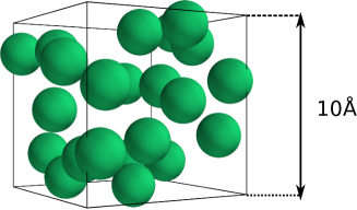
Figure 2: (Color online) 3D view of 2.6 Å diameter hard spheres randomly distributed in a 10x10x10 Å cube with a 3.6 Å mean spacing, as for liquid helium-4 at SVP. In helium, atoms are both strongly confined by hard core repulsion and dynamically delocalised by the zero point energy motion. Courtesy Nelle Varoquaux.

This large depletion raises the following question: how is it that the condensate fraction is only 8 % at $T$ = 0 while the superfluid fraction in the two-fluid model is 100 % ? The answer is simple: these are not the same quantities. The superfluid density stands for the inertia of the superfluid fraction, as measured for instance by a gyroscopic device sensitive to trapped superfluid currents (Reppy and Lane, 1965) or, less directly, by the decoupling of the superfluid component in an oscillating disk experiment (Andronikashvili and Mamaladze, 1966). In these experiments, only the elementary quasiparticles couple to the transverse oscillations of the cell walls; the remaining of the superfluid is not set into motion.

The superfluid fraction superfluid $\rho_{\mathrm{s}}/\rho$ is not directly related to the probability of finding bosons in the $\mathbf{k}=0$ quantum state. The occupation of the condensate is seen experimentally as a hump at zero energy transfer in the dynamic structure factor measured by neutron inelastic scattering (Glyde, 2013), a quantity rather well-hidden from experimentalists’sight in helium. When the superfluid is set into motion, the condensate enforces long-range order and drags the excited states along through the short-range correlations; there is entrainment of the atoms in the fluid by the condensate. Microscopic theory is needed to describe this process in detail.

Deferring to the end, §VIII.2, further discussion on the merits of, and differences between, the microscopic approach – the ODLRO concept of Penrose and Onsager (1956) and Yang (1962) – and the macroscopic quantum field point of view – a discussion found in Appendix A1 of Anderson (1966b) – the superfluid order parameter in ⁴He will be taken in the following as the macroscopic wavefunction Eq.(7), namely $\mathit{\Psi}(\mathbf{r})=f(\mathbf{r})\mathrm{e}^{\mathrm{i}\varphi(\mathbf{r})}$ with $f=n_{\mathrm{s}}^{{1/2}}$, $n_{\mathrm{s}}$ being the superfluid number density. This choice conforms to that of §I.2 and leads straightforwardly to the two-fluid model. The alternate choice to set $f=n_{0}^{{1/2}}$ would be less productive: the condensate density $n_{0}$ remains half-buried in the formalism and is difficult to access experimentally. This situation differs markedly from that in cold atomic gases. There, the condensate can be imaged directly in momentum space; it comprises most of the particles in the gas so that $n_{0}\simeq n$; the corresponding order parameter emerges seamlessly from perturbation theory applied to the weakly-interacting Bose gas following Bogolyubov’s prescriptions.

For weakly interacting bosons, the macroscopic wavefunction dynamics is governed by the Gross-Pitaevskii equation. The relevance of the Gross-Pitaevskii equation to the Bose-condensed systems has been put in a bright new perspective for ultra-cold atoms in a trap, for which it constitutes an excellent description (Dalfovo et al., 1999; Cohen-Tannoudji and Robilliard, 2001). However, the approach based on this equation turns out to be less adequate for the dense superfluid, sometimes not even qualitatively correct, as found for instance by Pomeau and Rica (1993) in the context of the breakdown of superflow. It will not be pursued here, except to mention that it does provide an estimate of the distance over which the two-fluid hydrodynamics needs to be supplemented by quantum corrections, as discussed in Sect.VII.

In all cases, the phase, a variable of lesser relevance in the older quantum mechanics, is now assigned the role of governing superfluid dynamics. A fundamental result, established early by Beliaev (1958), relates the phase of the condensate particles to the chemical potential, $\varphi=\mu\,t/\hbar$, where $t$ is time. The deep significance of this odd-looking relation only became apparent later, when the Josephson effects came on stage.

The role of the phase as a dynamical variable was extended to superfluid helium by Anderson (1964) (Anderson, 1965, 1966a, 1984) who noted that phase and particle number are canonically conjugate variables. This property is well-known in quantum electrodynamics for photons in a cavity. The number of photons in a given mode and their phase, defined for coherent electromagnetic fields in the cavity, are non-commuting operators. As such, they obey an uncertainty relation (Heitler, 1954) that reads:

$$\mbox{\small{d}\hskip 0.19376pt}N\,\mbox{\small{d}\hskip 0.19376pt}\varphi\sim 1\;.$$ (11)

As remarked by Heitler, “if the number of quanta of a wave are given it follows from eq.(11) that the phase of this wave is entirely undetermined and vice versa. If for two waves the phase difference is given (but not the absolute phase) the total number of light quanta may be determined, but it is uncertain to which wave they belong”. This remark will bear implications throughout this review.

Superfluidity is more than simply the absence of viscosity supplemented by the condition that vortices have quantised circulation. The urge to observe the role of the phase in a Josephson-type effect – and the failure to do so for a long period of time – became quite pressing to confirm the picture drawn by Anderson of helium as obeying quantum mechanics in a more profound way than simply as an ideal inviscid fluid with quantised velocity circulation.

I.5 Anderson’s phase slippage

Anderson’s famed “Considerations” on the flow of superfluid ⁴He (Anderson, 1966a) provided the conceptual basis for this experimental search for Josephson-type effects in neutral matter. Their underlying aim was to convey a physical, laboratory-oriented, meaning to order parameter Eq.(7) and, in particular, to its phase. These Considerations provided the groundwork for phase slippage experiments in ⁴He ; they were gradually fostered in a series of Lectures Notes (Anderson, 1964, 1965, 1984) and built upon the ideas of London (1954), Feynman (1955), and Penrose and Onsager (1956), and also on the quantum field theoretic approach of Beliaev (1958).

In the absence of a fully-established microscopic theory of dense boson systems, these considerations rest on the following set of well-argumented conjectures:

1. By extrapolation of the properties of the coherent photon fields in quantum electrodynamics recalled above, $N$ and $\varphi$ are taken in dense liquid helium as canonically conjugate dynamical (quantum) variables in the sense that $N\leftrightarrow\mathrm{i}(\partial/\partial\varphi)$ and $\varphi\leftrightarrow-\mathrm{i}(\partial/\partial N)$.

   As such, they obey the uncertainty relation (11). For a closed system with a fixed number of particles, the phase is completely undetermined. For the phase to be determined within $\mbox{\small{d}\hskip 0.19376pt}\varphi\ll 1$, $N$ must be allowed to vary, that is, the condensate must be able to exchange particles with other parts of the complete physical system, which includes the non-condensate fraction of the bosons and the eventual measuring apparatus.

   For the Josephson-effects experiments specifically considered by Anderson, the two weakly-coupled helium baths also exchange particles. For all these reasons, $N$ is allowed to fluctuate locally so that $\mbox{\small{d}\hskip 0.19376pt}N$ takes a non-zero value. It can be shown (Beliaev, 1958) that $\mbox{\small{d}\hskip 0.19376pt}N$ is of order $N$ rather than unity, so that $\mbox{\small{d}\hskip 0.19376pt}\varphi\sim{\cal O}(1/N)$ and $\varphi$ is well defined.

2. A Hamiltonian $\cal H$ should therefore exist such that, $N$ being free to vary,

   $$\hbar\frac{\partial N}{\partial t} = \mbox{ }\frac{\partial\cal H}{\partial\varphi}\;,$$ (12)

   $$\hbar\frac{\partial\varphi}{\partial t} = -\frac{\partial\cal H}{\partial N}\;.$$ (13)

   Upon coarse-graining, the quantum operators become quasi-classical and their coarse-grained average obey equations formerly identical to (12) and (13). Eq.(12) defines the particle current $J=\partial{E}/\hbar\partial\varphi$ since $\partial{\cal H}/\partial\varphi\Longrightarrow\partial E/\partial\varphi$ upon averaging. Likewise with $\partial{\cal H}/\partial N\Longrightarrow\partial E/\partial N=\mu+\kern 1.00006pt^{1}\kern-3.00003pt/\kern-1.00006pt_{2}m_{4}v_{\mathrm{s}}^{2}$ where $\mu$ is the chemical potential in the fluid at rest, namely $\mu=m_{4}P/\rho+m_{4}gh+s_{4}T$ with the usual notations, Eq.(13) becomes

   $$\hbar\frac{\partial\varphi}{\partial t}=-(\mu+\kern 1.00006pt^{1}\kern-3.00003pt/\kern-1.00006pt_{2}m_{4}v_{\mathrm{s}}^{2})\;.$$ (14)

   Eq.(14) states that, whenever there exists a chemical potential difference between two points 1 and 2 in a superfluid (or a superconductor), the phase of the order parameter varies in time with a rate proportional to $\mu_{1}-\mu_{2}$: this ac-effect is quite detectable and has nowadays many applications. It was first discussed by Josephson (1962) (Josephson, 1964) for the tunnelling current between superconductors coupled through a thin barrier. A full derivation for superfluid helium can be found in the monograph by Nozières and Pines.

   Upon taking the gradient of both left and right-hand sides, Eq.(13) becomes, using the definition (6) of $v_{\mathrm{s}}$,

   $$\frac{\partial v_{\mathrm{s}}}{\partial t}+\nabla\left(\frac{P}{\rho}+\frac{v_{\mathrm{s}}^{2}}{2}\right)=0\;,$$ (15)

   which is nothing else but the Euler equation for an inviscid fluid with no vorticity ($\boldsymbol{\omegaup}=\nabla\times\mathbf{v}_{\mathrm{s}}=0$). Equation (15) is precisely the same as that for the velocity of the superfluid component in Landau’s two-fluid hydrodynamics.

3. Anderson assumed that Eq.(14) for the time variation of the order parameter phase holds with no solution of continuity between the classical inviscid fluid case and the quantum tunnelling one and, i.e., that it has universal applicability. This unifying approach is, in a broad sense, internally consistent but details are missing of how the normal component interacts with the superfluid component, which brings dissipative terms into Eq.(15), and how the definition of $v_{\mathrm{s}}$ as $(\hbar/m)\,\nabla\varphi$ breaks down at small distances where coarse-graining cannot be performed. These fine points have been raised in the discussion at the end of Anderson’s communication at the Sussex Symposium on Quantum Fluids (Anderson, 1966b). His views are that the phase equation (14), being more fundamental than (15), always hold. This equation describes both simple superfluid acceleration, expressed by (15), the ideal tunnelling situation envisioned by Josephson (see Sect.VII), and when the variation of the phase is caused by the motion of vorticity.

4. The last conjecture asserts that the dissipation of the kinetic energy of a superflow is, when averaged over time, proportional to the rate at which vorticity crosses the superflow streamlines. In fact, a stronger statement has been rigorously proved by Huggins (1970), which governs the detailed transfer of energy between the potential flow of the superfluid and moving vorticity. This process is pivotal to the understanding of superflow decay and, more generally, of vortex dynamics as discussed in Sec.II.

Anderson’s ideas on phase slippage, linked to the motion of vortices, have provided the conceptual framework for the experiments on the onset of dissipation and the Josephson effects in superfluids, discussed below in Sect.III and VII.2. All facets of these experiments in superfluid ⁴He and ³He can be very well accounted for with the help of the macroscopic quantum phase $\varphi$. However, these ideas are still surrounded by an aura of mystery that lingers on in spite of the facts that: (1) the formal theoretical groundwork has been put on a firmer basis; (2) the implications of the uncertainty relation to laboratory observations, as well as of the other conjectures of Anderson, have been clarified by the developments of the experiments in the past forty and so years since they were formulated.

This review will tackle some of these advances, in particular, by showing what the phase slippage experiments really consist of, how phase slippage proceeds from a dissipative regime governed by vortex dynamics to a true dissipationless Josephson regime, and that this truly quantum behaviour manifests itself in matter waves interferometric measurements.

II Quantised vortex dynamics close to $T$=0

Vortex filaments are extended quasi-one-dimensional structures in the superfluid, line vortices. At the core of these defects, the superfluid order parameter is either zero as in ⁴He or heavily distorted as in ³He. They form the prevalent topological defects in superfluids.

At distances larger than the core size, superfluid vortices behave according to the laws of ideal fluid hydrodynamics, that is, as classical vortices with a given, quantised, vorticity. Classical vortices have been studied for many decades (Lamb, 1945; Saffman, 1992). Their properties have been the subject of detailed studies in recent years in order to clarify in a number of standing problems, their mass and impulse, the Magnus and Iordanski forces, the eigenmodes of isolated vortices - the Kelvin waves, the collective behaviour of vortex arrays - the Tkachenko waves, the reconnection of two vortices, superfluid vortex tangles, and lastly, the formation of vortices and their annihilation. This review is concerned mainly with the last topic but use will be made of other properties of vortices, either single or few at a time, mostly without consideration to the normal fluid background. These properties bear a close resemblance to those of magnetic vortices in superconductors as spelled out by Sonin and Krusius (1994).

At temperatures below 1 K, vortices in superfluid ⁴He experience negligible friction from the normal fluid, the fraction of which becomes very small. If they deform only little and slowly, they constitute stable fluid eddies: their velocity circulation is conserved (and furthermore, quantised) and they cannot vanish to nothing. Their core radius, $a_{0}$, is of the order of the superfluid coherence length, a few Å in ⁴He (Glaberson and Donnelly, 1986; Donnelly, 1991), one to two orders of magnitude larger in ³He depending on pressure (Vollhardt and Wölfle, 1990). As the temperature increases, the scattering of phonons and rotons by the vortex cores causes dissipation. Mutual friction between the superfluid vortices and normal fluid sets in. Close to the superfluid transition temperature, the core size increases and eventually diverges.

Some of the properties of vortices that have a relevance to phase slippage are summarised below. Extended coverage of this topic can be found in the monographs by Donnelly (1991) and by Sonin (2015). Here, the dynamical properties of superfluid vortices are derived directly from the existence of a superfluid order parameter. Some simplifying approximations are made in order to get a simpler physical description of a vortex element, treated more in the manner of a quasiparticle with mass, energy and impulse. The following discussion then rests on physical concepts such as energy conservation or the balance of forces. It follows largely the approach of Sonin (1987). It differs from the more traditional and rigorous fluid-mechanical approach, as can be found for instance in the monograph by Saffman (1992). It provides a more intuitive feel for the behaviour of superfluid vortices that will prove useful in the description of phase slips.

II.1 Quantisation of circulation

Superfluid vortices have quantised circulation. This property comes about because their core is non-superfluid: it disrupts the order parameter field and constitutes a topological defect in the superfluid. The circulation of the superfluid velocity $\mathbf{v}_{\mathrm{s}}$ on any path around such a defect,

$$\oint{\bf v_{\mathrm{s}}\cdot}{\mathrm{d}}{\mathbf{l}}=\frac{\hbar}{m_{4}}\,\oint\nabla\varphi\cdot{\mathrm{d}}{\mathbf{l}}$$ (16)

amounts to $\kappa_{4}=2\pi\hbar/m_{4}$  because the phase $\varphi$ of the order parameter can change only by multiples of $2\pi$ along any closed contour entirely located in the superfluid. This property holds for the true condensate wavefunction as a basic requirement of quantum mechanics. It is not altered in the coarse-graining average.

Consider the velocity circulation from point 1 to point 2 in Fig.3 along a path $\Gamma$ entirely located in the superfluid:

$$\kappa=\int_{1}^{2}{\bf v_{\mathrm{s}}.}{\mathrm{d}}{\bf l}=\frac{\hbar}{m_{4}}\int_{1}^{2}{\bf\nabla\varphi.}{\mathrm{d}}{\bf l}=\frac{\hbar}{m_{4}}(\varphi_{2}-\varphi_{1})\;.$$ (17)

Along another path $\Gamma^{\prime}$ also going from 1 to 2, as shown in Fig.3, the circulation is $(\hbar/m_{4})(\varphi_{2}-\varphi_{1}+2n\pi)$. If $\Gamma^{\prime}$ can be deformed into $\Gamma$ continuously while remaining in the superfluid, then $n=0$ . If this cannot be done, $n$ may be a non-zero integer, 1 in the case under consideration.

Thus, when path $\Gamma\textasciiacute$ crosses the core of a ⁴He vortex, in which superfluidity is destroyed and the order parameter amplitude goes to zero, $n$ changes by 1 because ⁴He vortices carry a single quantum of circulation for reasons discussed below. Conversely, when a vortex crosses a superfluid path from 1 to 2, the circulation along that path changes by one quantum and the phase difference by $2\pi$. This simple property forms the basis of the phase slip phenomenon described in Sec.III.

Figure 3: Two different situations for the path of integration in Eq.(17): (a) G can be deformed continuously into G’; both paths give the same phase difference between point 1 and point 2. (b)  vortex V stands between the two paths; the phase differences along G and G’ differ by $2\pi$.

Experiments have confirmed to a high accuracy the quantisation of hydrodynamic circulation both in ⁴He (Vinen, 1961; Whitmore and Zimmermann, Jr., 1968; Karn et al., 1980) and in ³He (Davis et al., 1991). This feature constitutes a cornerstone of superfluid physics, and evidence for the reality of the superfluid quantum phase.

II.2 Vortex flow field and line energy

The flow velocity induced by a straight vortex filament, chosen along the unit vector $\mathbf{\hat{z}}$, at a distance $\mathbf{r}$ measured in the plane perpendicular to $\mathbf{\hat{z}}$ is easily expressed from the quantisation of the velocity circulation and the symmetry around the vortex axis as

$$\oint\mathbf{v}\cdot\mathrm{d}\mathbf{l}=\kappa_{4}\;\Longrightarrow\;\mathbf{v}_{\mathrm{v}}=\frac{\kappa_{4}}{2\pi}\mathbf{\hat{z}}\times\frac{\mathbf{\hat{r}}}{r}\;,$$ (18)

provided that $r$ is larger than $a_{0}$. For $r\lesssim a_{0}$, the detailed structure of the core becomes important. The quantity $\mathbf{v}_{\mathrm{v}}$ is the vortical flow due to the vortex element. The superfluid velocity $\mathbf{v}_{\mathrm{s}}$ is the sum of an eventual potential flow $\mathbf{v}_{\mathrm{p}}$ existing independently of the vortex, for instance applied externally, and of $\mathbf{v}_{\mathrm{v}}$. The contribution of $\mathbf{v}_{\mathrm{p}}$ to the loop integral in Eq.(18) is nil and leaves the circulation unchanged. Straight vortex filaments are created by rotating the helium container; they have been the object of very detailed studies.

Equation (18) can be extended to curved vortices, provided that their radii of curvature are much larger than the core radius $a_{0}$. It bears a direct analogy with Ampère’s law, $\mathbf{v}$ standing for the magnetic field and $\kappa$ for the electric current carried by the conductor. The velocity at point $\mathbf{r}$ induced by a closed vortex filament lying along the curve $\mathbf{s}$ is then given by the analogue of the Biot-Savart law in electrodynamics:

$$\mathbf{v}_{\mathrm{v}}(\mathbf{r})=\frac{\kappa_{4}}{4\pi}\oint\mathrm{d}\mathbf{l}\times\frac{\mathbf{r}-\mathbf{s}(l)}{|\mathbf{r}-\mathbf{s}(l)|^{3}}\;.$$ (19)

The geometrical representation of the vortex loop by $\mathbf{s}$ is such that $\mathrm{d}\mathbf{l}=\mathrm{d}\mathbf{s}$ is a vector oriented along the tangent to the loop $\mathbf{\hat{t}}$ of infinitesimal length $\mathrm{d}l$, $l$ being the arc length of the loop (see the sketch in Fig.4). The tangent $\mathbf{\hat{t}}$ is the unit vector $\mathrm{d}\mathbf{s}/\mathrm{d}l=\mathrm{d}\mathbf{l}/\mathrm{d}l$. Its derivative with respect to $l$ defines the normal to the loop $\mathbf{\hat{n}}$ and the radius of curvature $R$: $\mathrm{d}\mathbf{\hat{t}}/\mathrm{d}l=\mathrm{d}^{2}\mathbf{s}/\mathrm{d}l^{2}=\mathbf{\hat{n}}/R$. As noted above, the radius of curvature $R$ should be large – and the change of orientation of the tangent $\mathrm{d}\mathbf{\hat{t}}/\mathrm{d}l$ small – with respect to the core radius for this representation of the vortex element as a one-dimensional line to be valid.

The integrand in Eq.(19) gives the contribution of the vortex element $\mathrm{d}\mathbf{l}$ located at $\mathbf{s}$ on the loop to the full velocity field. An integration by parts yields

$$\mathbf{v}_{\mathrm{v}}(\mathbf{r})=\frac{\kappa_{4}}{4\pi}\nabla\times\oint\frac{\mathrm{d}\mathbf{l}}{|\mathbf{r}-\mathbf{s}(l)|}=\nabla\times\mathbf{A}(\mathbf{r})\;,$$ (20)

which defines a vector potential for the vortex velocity field, $\mathbf{v}_{\mathrm{v}}=\nabla\times\mathbf{A}$.

Equation (20) fulfils the mantra of conventional mathematical physics according to which a vector field can be split into an irrotational part, which derives from a scalar potential, and a remainder, the solenoidal part, which is not curl-free and which derives from a vector potential.

While utterly correct in mathematical terms, this point of view may be slightly misleading for the superfluid velocity fields. The latter are a subset only of the more general vector fields in the sense that vorticity is localised in space to the vortex cores and that the vortex line can be treated as a line singularity. The Biot-Savart law (19) can then be put under the following form

$$\mathbf{v}_{\mathrm{v}}(\mathbf{r})=\frac{\kappa_{4}}{4\pi}\,\nabla_{\mathbf{r}}\,\left\{\iint_{S}\frac{\mathbf{r}-\mathbf{R}}{|\mathbf{r}-\mathbf{R}|^{3}}\cdot\mathrm{d}\mathbf{S}\right\}=\frac{\hbar}{m_{4}}\,\nabla\varphi_{\mathrm{v}}\;,$$ (21)

the infinitesimal surface element $\mathrm{d}\mathbf{S}$ being located at position $\mathbf{R}$. Thus the velocity fostered by the vortex derives from a scalar potential as well as a vector potential. Everywhere in the superfluid but at the precise location of the vortex cores, the superfluid velocity $v_{\mathrm{s}}$ is indeed irrotational and derives from a scalar potential, the quantum phase.

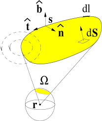
Figure 4: (Color online) The geometrical representation of a vortex loop, an arbitrary surface $S$ spanning the loop, with element $\mathrm{d}\mathbf{S}$, and the solid angle $\Omega$ subtended by the loop from point $\mathbf{r}$, the tangent $\mathbf{\hat{t}}$, normal $\mathbf{\hat{n}}$, and binormal $\mathbf{\hat{b}}$ at point $\mathbf{s}$. The flow lines of the vortex velocity field (dashed line) thread surface $S$ where the phase changes determination by $2\pi$. Solid angle $\Omega$ offers a geometrical representation of the integrand in Eq.(21).

The velocity induced by a vortex loop decreases at large distance from the loop as that of a dipole in the electromagnetic analogy, that is as $1/r^{3}$, much faster than the $1/r$ dependence for straight vortex filaments (see Eq.(18)). The $1/r$ dependence can still be expected to hold at a distance away from the core smaller than the local radius of curvature of the vortex filament. At distances larger than the loop size, the velocity field rapidly dies away. This property is well known for magnetic fields generated by electric current loops. It means, for practical purposes, that vortex loops far apart interfere very weakly and that distant boundaries have negligible effect. These simplifying features will often be assumed in the following.

II.2.1 Vortex line energy

The flow around the core of a vortex element carries kinetic energy, obtained by integration of $\int(1/2)\rho_{\mathrm{s}}v^{2}_{\mathrm{v}}{\mathrm{d}}\tau\,$ over the volume $V$ in which this flow extends. The quantity $\rho_{\mathrm{s}}$ is the superfluid density. This integral is evaluated by introducing the vector potential $\mathbf{A}$, Eq.(20), from which derives the vortical flow field, as follows:

$$\begin{split}E_{\mathrm{v}}&=\frac{\rho_{\mathrm{s}}}{2}\,\int_{\mathrm{V}}\!\!\mathrm{d}\tau\,\mathbf{v}_{\mathrm{v}}\cdot\mathbf{v}_{\mathrm{v}}=\frac{\rho_{\mathrm{s}}}{2}\,\int_{\mathrm{V}}\!\!\mathrm{d}\tau\,\mathbf{v}_{\mathrm{v}}\cdot\nabla\times\mathbf{A}\\ &=\frac{\rho_{\mathrm{s}}}{2}\,\int_{\mathrm{V}}\!\!\mathrm{d}\tau\,\nabla\cdot(\mathbf{A}\times\mathbf{v}_{\mathrm{v}})+\frac{\rho_{\mathrm{s}}}{2}\,\int_{\mathrm{V}}\!\!\mathrm{d}\tau\,\mathbf{A}\cdot(\nabla\times\mathbf{v}_{\mathrm{v}})\;.\end{split}$$

The last line is obtained with the help of vector identity $\nabla\cdot(\mathbf{a}\times\mathbf{b})=\mathbf{b}\cdot(\nabla\times\mathbf{a})-\mathbf{a}\cdot(\nabla\times\mathbf{b})$. It consists of the sum of two volume integrals. The first can be changed into a surface integral over $\mathbf{A}\times\mathbf{v}$ with the divergence theorem. By taking the volume boundary sufficiently far from the vortex element, supposed isolated in a large volume, the surface integral can be made negligible. In the second integral, the curl of $\mathbf{v}_{\mathrm{v}}$ is zero everywhere but on the vortex core, where it is singular: $\nabla\times\mathbf{v}_{\mathrm{v}}=\kappa_{4}\,\mathbf{\hat{t}}\,\delta_{2}(\mathbf{r}-\mathbf{s})$. Integration over the two-dimensional delta function $\delta_{2}(\mathbf{x})$, defined in the plane normal to the tangent $\mathbf{\hat{t}}$ to the loop, reduces this volume integral to a line integral over the vortex element:

$$E_{\mathrm{v}}=\frac{\rho_{\mathrm{s}}\kappa_{4}}{2}\,\oint\mathrm{d}\mathbf{l}\cdot\mathbf{A}\;.$$ (22)

The vortex kinetic energy is the circulation of the vector potential along the the vortex filament.

By substitution of the expression (20) for the vector potential $\mathbf{A}$ in Eq.(22), the vortex energy can be expressed by a double contour integral over the vortex loop:

$$E_{\mathrm{v}}=\frac{\rho_{\mathrm{s}}\kappa_{4}^{2}}{8\pi}\,\oint\!\!\oint\frac{\mathrm{d}\mathbf{s}(l_{1})}{\mathrm{d}l_{1}}\cdot\frac{\mathrm{d}\mathbf{s}(l_{2})}{\mathrm{d}l_{2}}\frac{\mathrm{d}l_{1}\,\mathrm{d}l_{2}}{\left|\mathbf{s}(l_{1})-\mathbf{s}(l_{2})\right|}\;.$$ (23)

Because $E_{\mathrm{v}}$ in Eq.(23) varies as $\kappa_{4}^{2}$, loops carrying two quanta of circulation would have four times the line energy of single charge ones. Vortices with multiple quanta of circulation are thus strongly disfavoured on energy grounds compared to separate singly-charged vortices with the same total vorticity charge; they are energetically unstable and decay spontaneously into several singly-charged entities. Only loops and filaments carrying one quantum of circulation are considered here.

For a circular ring of radius $R$ the integral can be evaluated in terms of elliptic functions and expanded in terms of the small parameter $a_{0}/R$. The kinetic energy associated with the ring velocity field is then given by

$$E_{\mathrm{R}}=\frac{1}{2}\rho_{\mathrm{s}}\kappa_{4}^{2}R\,\ln\frac{8R}{a_{0}}+{\cal O}\left(\frac{a_{0}}{R}\right)\;.$$ (24)

For a straight vortex filament, the integral for the kinetic energy in the volume comprised between two planes perpendicular to the filament stems out directly from Eq.(18). For a unit length of vortex the result reads:

$${\mathsf{\epsilon}}_{\mathrm{f}}=\frac{\rho_{\mathrm{s}}\kappa_{4}^{2}}{4\pi}\ln\left(\frac{r_{\mathrm{m}}}{a_{0}}\right)\;.$$ (25)

The logarithmic divergence is cut at short distance to $a_{0}$, taken as the definition of the core radius. Its value, of the order of one Å  at low pressure, is obtained from experiment (Rayfield and Reif, 1964). The far distance cut-off $r_{\mathrm{m}}$ is the minimum distance over which the vortex flow field is undisturbed: it is the smallest of 1) the size of the container, 2) the average radius of curvature of the vortex, 3) the distance to neighbouring vortices. For ångström-size vortices, taking $r_{\mathrm{m}}/a_{0}=10$, ${\mathsf{\epsilon}}_{\mathrm{v}}\sim 2$ kelvin per ångström: vortices are high-energy excitations of the superfluid as compared to thermal excitations, phonons or rotons. Changes in $r_{\mathrm{m}}$ along the vortex line are disregarded because they enter logarithmic terms and yield small corrections only for $r_{\mathrm{m}}\gg a_{0}$: when the vortex deforms, its energy changes mostly as its length, and little with its shape.

The line energy of the core, usually taken as

$${\mathsf{\epsilon}}_{\mathrm{sb}}=-\frac{7}{4}\,\frac{\rho_{\mathrm{s}}\kappa_{4}^{2}}{4\pi}\;,$$

for a core rotating as a solid body, must be added to Eq.(25) to obtain the full vortex energy per unit length

$$\mathsf{\epsilon}_{\mathrm{v}}=\mathsf{\epsilon}_{\mathrm{f}}\,+\,\mathsf{\epsilon}_{\mathrm{sb}}=\frac{\rho_{\mathrm{s}}\kappa_{4}^{2}}{4\pi}\left\{\ln\left(\frac{r_{\mathrm{m}}}{a_{0}}\right)-\frac{7}{4}\right\}\;.$$ (26)

The full energy of a curved vortex line is thus approximated by $\mathsf{\epsilon}_{\mathrm{v}}$ times its total length. For instance, the energy of a vortex ring, Eq.(24), stems from Eq.(25) if $r_{\mathrm{m}}$ is taken to be $8R$.

Expression (26) holds for straight vortex lines, rings, curved filaments or general loops provided than $r_{\mathrm{m}}\gg a_{0}$. It can be viewed as a force developing along the vortex axis, a line tension that tends to shorten the vortex length. That is, the vortex line pulls on its ends: if an end becomes loose it shrinks to zero. Stable vortices in finite size containers either are closed on themselves in loops or connect to the container walls.

II.2.2 Stable vortices

It follows from the existence of a positive line tension that a vortex loop would tend to spontaneously reduce its length and minimise the line energy. However, the energy so released by the vortex loop in its motion can be disposed of into the surrounding fluid only in certain conditions of flow. The line tension is opposed by other forces that arise from the vortex motion in the fluid or from its interaction with the boundaries, namely, the Magnus force and pinning forces.

As stand-alone loops or pinned filaments, their length is constant as long as they cannot exchange energy with the rest of the fluid (or the external world). In the presence of hard walls, their flow field must be such as to satisfy the condition that no fluid can penetrate into the wall. A convenient way of satisfying such a boundary condition is to continue the vortex filament into the wall, forming an imaginary image vortex. Such a continuation procedure can be shown to be possible and to yield a unique velocity field. Vortices meeting with walls usually satisfy the condition of no flow through a solid boundary by standing perpendicular to it. Thus, finite length vortices always close on themselves or end at walls. In this latter case, they also form closed loops if their image is taken into account. The opposite view, namely that vortices are most of the time infinitely long as, for instance, vortices formed under rotation in a cylindrical helium bucket, is also held. The process of nucleation of vortices considered below obviously requires that their size be finite (otherwise, the energy involved would be infinite): the isolated vortex loops dealt with in the following have a finite size, usually small.

II.2.3 Vortex line impulse

If an external potential flow with velocity $\mathbf{v}_{\mathrm{p}}=(\hbar/m_{4})\,\nabla\varphi_{\mathrm{p}}$ imposed by moving boundaries, a piston for instance, or by nearby vortices, the kinetic energy of the combined flow $\mathbf{v}_{\mathrm{p}}+\mathbf{v}_{\mathrm{v}}$ in a given volume $V$ is the sum of the kinetic energy of the remotely applied superflow $\mathbf{v}_{\mathrm{p}}$, that of the vortex loop, obtained from Eq.(23), and the volume integral of the cross term of the scalar product of $\mathbf{v}_{\mathrm{p}}$ and $\mathbf{v}_{\mathrm{v}}$. This last term reads

$$E_{\mathrm{\,I}}=\rho_{\mathrm{s}}\int_{V}\mathbf{v}_{\mathrm{p}}\cdot\mathbf{v}_{\mathrm{v}}\,\mathrm{d}\tau=\rho_{\mathrm{s}}\,\frac{\hbar^{2}}{m_{4}^{2}}\int_{V}\nabla\varphi_{\mathrm{p}}\cdot\nabla\varphi_{\mathrm{v}}\,\mathrm{d}\tau\;,$$ (27)

and represents the energy of interaction between the vortex and the applied flow. Making use of Green’s first identity, the integral in Eq. (27) can be rewritten as

$$E_{\mathrm{\,I}}=\rho_{\mathrm{s}}\frac{\hbar}{m_{4}}\int_{S}\varphi_{\mathrm{v}}\,\mathbf{v}_{\mathrm{p}}\cdot\mathrm{\,}d\mathbf{S}\;,$$ (28)

where $\varphi_{\mathrm{v}}$ is the phase change contributed by the vortex own flow field.

The bounding surface $S$ yields not one but two contributions to the integral in Eq.(28), the outer surface bounding $V$ and, quite importantly, the cut spanning the vortex loop over which $\varphi_{\mathrm{v}}$ changes discontinuously by $2\pi$ (see Fig.4). If $V$ can be chosen large enough, the velocity induced by the vortex on its surface is negligible and $\varphi_{\mathrm{v}}$ is a constant: the contribution to Eq.(28) of the outer surface reduces to the net flux of $\mathbf{v}_{\mathrm{p}}$, which is zero. The contribution of the cut is $2\pi$ times the flux of $\mathbf{v}_{\mathrm{p}}$ through the vortex loop. Introducing the mass flux of the applied potential flow through the vortex loop, $J_{\mathrm{p}}$, the contribution of the cross term (27) takes the very simple form

$$E_{\mathrm{\,I}}=\rho_{\mathrm{s}}\frac{2\pi\hbar}{m_{4}}\int_{\mathrm{loop}}\mathbf{v}_{\mathrm{p}}\cdot\,\mathrm{d}\mathbf{S}=\kappa_{4}J_{\mathrm{p}}\;.$$ (29)

Thus, an applied flow contributes to the vortex loop energy by the additional mass flux $J_{\mathrm{p}}$ that it causes through the loop times the quantum of circulation. This result will be derived below in §II.3 from the more general phase-slippage theorem governing the exchange of energy between potential and vortical flows.

In the event that $\mathbf{v}_{\mathrm{p}}$ can be considered as constant over the surface spanned by the vortex loop, Eq.(29) becomes even simpler:

$$E_{\mathrm{\,I}}=\rho_{\mathrm{s}}\kappa_{4}\mathbf{S}\cdot\mathbf{v}_{\mathrm{p}}\;,$$ (30)

in which $\mathbf{S}$ is the vectorial area of the loop, $\int\mathrm{d}\mathbf{S}=(1/2)\,\oint\mathbf{r}\times\mathrm{d}\mathbf{l}$, $\mathrm{d}\mathbf{l}$ being the line element at point $\mathbf{s}$ of the oriented loop.

The total energy of the vortex immersed in an applied flow field is the sum of its energy in the rest frame, $E_{0}$, given by Eq.(23), and the energy of interaction with the potential flow, $E_{\mathrm{\,I}}$. For Eq.(30), this reads

$$E_{\mathrm{v}}=E_{0}+\mathbf{P}\cdot\mathbf{v}_{\mathrm{p}}\;,{\mbox{ with }}\mathbf{P}=\rho_{\mathrm{s}}\kappa_{4}\mathbf{S}\;,$$ (31)

where $\mathbf{P}$ ican be defined as the impulse of the vortex loop.

For a circular loop of radius $R$, a vortex ring, Eq.(31) gives the well-known result (Lamb, 1945):

$$P_{\mathrm{R}}=\pi\rho_{\mathrm{s}}\kappa_{4}R^{2}\;.$$ (32)

It emerges from this derivation (and the various approximations made along the way) that, under a Galilean boost, vortex loops do behave as Landau quasiparticles, with an energy proportional to their length and an impulse proportional to their area. This approach puts some flesh on the bare bones of the conventional (and exact) fluid-mechanical vortex dynamics; it gives substance to the intuitive view than they can be treated as independent elementary entities. This physically meaningful manner of separating the vortical flow from the local value of the remotely potential superflow $v_{\mathrm{p}}$ will prove quite useful in the following.

II.2.4 Vortex self-velocity

The impulse is not simply a plain geometrical quantity as Eqs.(30) or (31) would let think. It is the resultant of the impulsive pressures that must be applied to the fluid at rest to create the vortex loop from rest. It possesses some of the properties of a true momentum. For instance, the propagation velocity of the vortex ring, Eq.(34), can be expressed as the group velocity associated with the energy (24) and impulse (32) (Langer and Reppy, 1970; Roberts and Donnelly, 1970):

$$v_{\mathrm{R}}=\frac{\mathrm{d}E_{\mathrm{R}}}{\mathrm{d}P_{\mathrm{R}}}=\frac{\kappa_{4}}{4\pi R}\,\left(\ln\frac{8R}{a_{0}}-\frac{3}{4}\right)\;,$$ (33)

Expression (33) tends asymptotically to the actual velocity of a ring with a hollow core as computed directly from the Biot and Savart law, which moves along its symmetry axis $\hat{\mathbf{n}}$ with velocity

$$\frac{\mathrm{d}\mathbf{s}}{\mathrm{d}t}=\mathbf{v}_{\mathrm{R}}=\frac{\kappa_{4}}{4\pi R}\,\left(\ln\frac{8R}{a_{0}}-\frac{1}{4}\right)\hat{\mathbf{n}}\;.$$ (34)

However, these simple properties do not imply that a vortex has actual linear momentum. The vortical impulse is more elusive. For instance, it can be shown that a vortex ring moving freely under its own force at velocity $v_{\mathrm{R}}$ and impinging on a wall exerts no force on it (Fetter, 1972). This somewhat counter-intuitive result arises from the distribution of the flow around the vortex loop (Cross, 1974). The contribution of the flow that goes in the forward direction, and which causes the ring free motion, does impart a momentum impulse into the wall equal to $P_{\mathrm{R}}$, but the returning fluid away from the ring, the backflow, yields an opposite contribution that leads to full cancellation of the momentum transfer recorded over an infinitely extended wall for the complete collision event. This push and pull action constitutes a reminder that actual momentum is carried by the individual fluid elements and that a vortex is a hydrodynamical object made up of many of those elements.

Isolated circular rings propagate undistorted under their own velocity field in the superfluid at rest for symmetry reasons.. Only a few vortex shapes propagate undistorted in their own velocity field. Straight vortex pairs and helical vortices are other examples (Langer and Reppy, 1970).

For an arbitrarily curved vortex, the self-velocity of each curve element can be approximated by Eq. (34), $R$ being replaced by the local radius of curvature, $r_{\mathrm{m}}=|\mathrm{d}^{2}\mathbf{s}/\mathrm{d}\xi^{2}|^{-1}$, parameter $\xi$ being the line length of the curve represented by $\mathbf{s}(\xi)$. The validity of this “local induction” approximation, which requires that $r_{\mathrm{m}}$ be large with respect to the vortex core radius, has been discussed in particular by Schwarz (1978, 1985) who has used it in extensive numerical simulations of 3D vortex motion.

II.2.5 The vortex mass

The impulse of a vortex discussed above is in no way related to the vortex self-velocity as the product of this velocity by an inertial mass. The problem of the mass of a vortex has been a long lasting riddle, which has now been resolved in a satisfactory way in superfluid ⁴He.

This mass arises from several contributions. If it is assumed that the vortex has a hollow core of radius $a_{0}$ and that the compressibility of the surrounding superfluid in rapid rotation can be neglected, the vortex mass is simply the mass of the displaced fluid. For a cylindrical body, this amounts to $\pi\rho_{\mathrm{s}}a_{0}^{2}$ per unit length, a standard result of classical fluid dynamics Lamb (1945). The minuteness of $a_{0}$ in ⁴He, $1\sim 2$ Å, of the same order as the interparticle spacing, makes this contribution very small.

However, compressibility cannot be neglected in the vicinity of the vortex core because the peripheral velocity, Eq.(18), becomes large. The corresponding pressure drop is given by the Bernoulli equation:

$$\frac{\mbox{\small{d}\hskip 0.19376pt}P}{\rho_{\mathrm{s}}}=-\frac{1}{2}\mbox{\small{d}\hskip 0.19376pt}(v^{2}_{\mathrm{s}})=0\;.$$ (35)

The change in density at distance $r$ from the core where the velocity is $\kappa_{4}/2\pi r$ is then:

$$\mbox{\small{d}\hskip 0.19376pt}\rho_{\mathrm{s}}=\frac{\mbox{\small{d}\hskip 0.19376pt}P}{c_{1}^{2}}=\frac{\kappa_{4}^{2}}{8\pi^{2}}\,\frac{\rho_{s}}{c_{1}^{2}}\,\frac{1}{r^{2}}\;,$$ (36)

using the relation between the (first) sound velocity and the compressibility $c_{1}=(\partial P/\partial\rho)^{-1/2}$, which is justified when the normal fluid fraction is small ($\rho_{\mathrm{s}}\simeq\rho$). The overall change of mass about a unit length of vortex filament arising from the fluid compressibility is obtained by integrating Eq.(36) over space:

$$\mu_{\mathrm{v}}=\int_{a_{0}}^{r_{\mathrm{m}}}\!\!\int_{0}^{2\pi}\!\!\int_{0}^{1}\mbox{\small{d}\hskip 0.19376pt}\rho_{\mathrm{s}}r\mathrm{d}r\mathrm{d}\theta\mathrm{d}z=\frac{\kappa_{4}^{2}}{4\pi}\,\frac{\rho_{s}}{c_{1}^{2}}\,\ln\frac{r_{\mathrm{m}}}{a_{0}}\;.$$ (37)

The vortex mass per unit length $\mu_{\mathrm{v}}$diverges logarithmically with $r_{\mathrm{m}}$ and ranges from negligible for $r_{\mathrm{m}}\sim$ a few core radii to important for large vortices, $r_{\mathrm{m}}/a_{0}\gtrsim 10^{3}$. However, in most cases, the mass of the vortex remains small and can be neglected except for high frequency phenomena (Baym and Chandler, 1983; Sonin, 1987) and, possibly, for quantum tunnelling (Volovik, 1997).

The Bernoulli effect, Eq.(36), also causes ³He impurities and ions to be trapped on the vortex cores because their chemical potential decreases with the ⁴He density. They prefer to sit in low density regions of the fluid. Trapped impurities add their own inertial mass $m_{\mathrm{I}}$ to that of the core. In superfluid ³He, the core is large and yields the dominant contribution to the vortex mass (Kopnin, 1978, 1995; Duan and Leggett, 1992; Volovik, 1997).

II.3 Energy exchange between potential and vortical flows

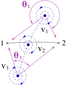
Figure 5: (Color online) Stream of vortices $\mathrm{v}_{1}$, $\mathrm{v}_{2}$, $\mathrm{v}_{3}$, …  crossing a path between point 1 and point 2, moving from bottom to top. The vortices are represented by dots and are assumed perpendicular to the figure and nearly straight in the vicinity of 1-2. Each contributes angle $\theta_{i}$ to the phase difference recorded between 1 and 2. In its travel from far below to far above line 1-2, each vortex contributes $2\pi$ to the phase difference. According to the ac Josephson effect, a pressure difference develops in the superfluid due to the stream of vortices (see Eq.(38).

Following the insight of Anderson (1966b), the idea that phase slippage by moving vorticity causes dissipation in superfluids and superconductors has become conventional wisdom. If, referring for instance to the situation of Fig.5, there is not just one vortex as in Fig.3 but a constant stream of vortices crossing the path 1-2 at a rate of $n$ per second, driven by some external force, a pressure difference develops in the superfluid according to the Josephson ac-relation (14). When the superfluid is free to move, it is accelerated by the cross stream of vortices: work is done onto the superfluid by the applied external force, for instance an electric field acting on charges trapped in the vortex cores. This Section dwells on the mechanism for this exchange of energy between the purely potential superflow and vorticity.

Anderson (1966b) noted in an appendix entitled “A ‘new’ corollary in classical hydrodynamics” that, whenever there exists a steady stream of vortices, for instance at the mouth of an orifice, the quantum phase in the superfluid would change there at a constant rate and, according to Eq.(14), the following chemical potential difference would build up

$$\hbar\frac{\mathrm{d}n_{\mathrm{vortices}}}{\mathrm{d}t}\Big{|}_{1}^{2}=\bigg{<}\hbar\,\frac{\mathrm{d}(\varphi_{2}-\varphi_{1})}{\mathrm{d}t}\bigg{>}=\big{<}\mu_{2}-\mu_{1}\big{>}\;.$$ (38)

In Eq.(38), the brackets stand for time-averaging and the quantity $\mathrm{d}n_{\mathrm{vortices}}/\mathrm{d}t$ for the rate of passage of vortices across a line joining points 1 and 2, as depicted in Fig.5.

This result is of no special importance in classical hydrodynamics because the velocity circulation carried by each vortex, albeit constant, can take any value, while in the superfluid it is directly related to the phase of the macroscopic wavefunction and quantised . A formal proof of this conjecture, based on the standard decomposition of any vector field into an irrotational contribution and a solenoidal one was given by Huggins (1970). The following derivation is based on the more physical approach to vortex dynamics, which makes use of the concepts of force and energy.

II.3.1 The Magnus force

Consider the interaction energy between a vortex loop and a potential flow $\mathbf{v}_{\mathrm{p}}$, Eq.(30). Under an infinitesimal displacement $\mbox{\small{d}\hskip 0.19376pt}\mathbf{x}$ of a small line element $\Delta\mathbf{l}$, as shown in Fig.6, the energy of the vortex loop changes according to

$$\mbox{\small{d}\hskip 0.19376pt}(\Delta E_{\mathrm{I}})=\kappa_{4}\rho_{\mathrm{s}}\,\mbox{\small{d}\hskip 0.19376pt}\mathbf{x}\times\Delta\mathbf{l}\cdot\mathbf{v}_{\mathrm{l}}=\kappa_{4}\rho_{\mathrm{s}}\,\Delta\mathbf{l}\times\mathbf{v}_{\mathrm{l}}\cdot\mbox{\small{d}\hskip 0.19376pt}\mathbf{x}\;,$$ (39)

where $\mathbf{v}_{\mathrm{l}}$ is the local superflow velocity as seen by the vortex element standing still. The local flow velocity $\mathbf{v}_{\mathrm{l}}$ is the sum of the applied superflow $\mathbf{v}_{\mathrm{p}}$ and the flow induced by the other parts of the vortex loop, $\mathbf{v}_{\mathrm{v}}$. Equation (39) expresses the functional derivative $\mbox{\small{d}\hskip 0.19376pt}(\Delta E_{\mathrm{I}})/\mbox{\small{d}\hskip 0.19376pt}\mathbf{x}$ of the energy with respect to an infinitesimal deformation of the vortex line.

Figure 6: Virtual displacement by $\mbox{\small{d}\hskip 0.19376pt}x$ of a small line element $\Delta l$.

If the vortex loop moves along at velocity $\mathbf{v}_{\mathrm{loop}}$ together with the element under consideration in the rest frame of the observer, $\mathbf{v}_{\mathrm{l}}$ in Eq.(39) becomes $\mathbf{v}_{\mathrm{l}}-\mathbf{v}_{\mathrm{loop}}$ and this force takes the same form as the Magnus force for a line vortex in classical hydrodynamics with a fluid density $\rho_{\mathrm{s}}$: 

$$\frac{\mbox{\small{d}\hskip 0.19376pt}(\Delta E_{\mathrm{I}})}{\mbox{\small{d}\hskip 0.19376pt}\mathbf{x}}=\Delta\mathbf{F}_{\mathrm{M}}=\kappa_{4}\rho_{\mathrm{s}}(\mathbf{v}_{\mathrm{loop}}-\mathbf{v}_{\mathrm{l}})\times\Delta\mathbf{l}\;,$$ (40)

The Magnus force, Eq.(40), has a simple physical origin. It is due to the Bernoulli effect that arises from the rotational flow around the vortex core. As shown in Fig.7, this flow adds to the potential flow in the lower half-plane and subtracts from it in the upper half-plane. Integrating the resulting pressure difference obtained from the Bernoulli Eq.(35) over the cylinder yields a downward force expressed by Eq.(40).

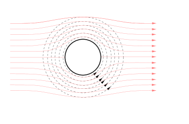
Figure 7: (Color online) Potential streamlines past the cylindrical vortex core flowing from left to right in thin plain lines. The flow from the vortex, in dashed lines, subtracts from the potential flow in the upper half and adds to it in the lower half, inducing a Bernoulli pressure difference between top and bottom.

The Magnus force on each element of the vortex line arises ultimately from momentum conservation in the fluid and comes into play whenever the vortex trajectory differs from that of the local fluid particles. When no other force acts on the vortex core (such as, e.g., an electric field on charges trapped in the core, or friction from the normal fluid component, …) $\mathbf{F}_{\mathrm{M}}$ must be zero, hence $\mathbf{v}_{\mathrm{loop}}=\mathbf{v}_{\mathrm{l}}$: the vortex core moves with the local superfluid velocity. The velocity of the core at point ${\mathbf{s}}$ is the sum of the velocity of the local potential flow ${\mathbf{v}}_{\mathrm{p}}$ at ${\mathbf{s}}$ when there is no vortex, and of the velocity ${\mathbf{v}}_{\mathrm{v}}$ induced at ${\mathbf{s}}$ by the other parts of the vortex. If no flow is applied, $\mathbf{v}_{\mathrm{p}}=0$, then $\mathbf{v}_{\mathrm{loop}}=\mathbf{v}_{\mathrm{v}}$: the vortex loop moves under its own flow field in the superfluid at rest at large distance. The vortex thus appears to behave as a quasiparticle in its own right although it stands only for the vortical part of the total flow. The physical picture that emerges from this approach rings a familiar bell to condensed matter physicists.

II.3.2 Quantised vorticity and the Kelvin-Helmholtz theorem

That free vortex loops moves with the local fluid particles conforms to the Kelvin-Helmholtz theorem. This result has been obtained here as a consequence of the quantisation of circulation, Eq.(18). The Kelvin-Helmholtz theorem is usually derived from the Euler equation and the implicit assumption that the motion of the fluid is isentropic (Landau and Lifshitz, 1959). A further implicit assumption is that the velocity field and the loop deformation are well-behaved analytically, that is, continuous in space and time. The relevance of these remarks will become apparent in Sect.V.1 on vortex nucleation, which deals with the spontaneous appearance of vorticity, in other words, the violation of the Kelvin-Helmholtz theorem. The derivation given above does not hide these fine points under the rug; it explicitly rests on the quantisation of circulation, hence its conservation, and also implies isentropic and continuous superfluid motion. When this fails new phenomena occur: vortices may be nucleated.

As the effect of external forces and mutual friction has been set aside for simplicity, no work is done on the vortex itself except by the interaction with the local superflow. Thus any gain or loss of energy by the vortex balances that lost or gained by the potential flow. The way by which this conservation of energy proceeds is instructive; the detailed analysis is given in the following.

II.3.3 The phase slippage theorem

If $\mbox{\small{d}\hskip 0.19376pt}\mathbf{x}$, used in Eq.(39) as a virtual displacement to compute the forces acting on $\Delta\mathbf{l}$, becomes a real displacement $\mathbf{v}_{\mathrm{loop}}\Delta\mathrm{t}$, actual work during the time $\Delta\mathrm{t}$ is done by the applied potential flow on the vortex loop. The energy balance is expressed by rewriting Eq.(39) as

$$\begin{split}\mbox{\small{d}\hskip 0.19376pt}(\Delta E_{\mathrm{I}})&=\kappa_{4}\rho_{\mathrm{s}}\,\Delta\mathbf{l}\times(\mathbf{v}_{\mathrm{p}}+\mathbf{v}_{\mathrm{v}})\cdot\mbox{\small{d}\hskip 0.19376pt}\mathbf{x}\\ &=\kappa_{4}\rho_{\mathrm{s}}\,\Delta\mathbf{l}\times\mathbf{v}_{\mathrm{p}}\cdot\mathbf{v}_{\mathrm{loop}}\Delta t+\kappa_{4}\rho_{\mathrm{s}}\,\Delta\mathbf{l}\times\mathbf{v}_{\mathrm{v}}\cdot\mathbf{v}_{\mathrm{loop}}\Delta t\;.\end{split}$$ (41)

In free motion – disregarding friction of the core on the normal component and with no force applied externally – the vortex loop follows the fluid stream: $\mathbf{v}_{\mathrm{loop}}=\mathbf{v}_{\mathrm{l}}=\mathbf{v}_{\mathrm{p}}+\mathbf{v}_{\mathrm{v}}$. The triple products are equal in magnitude and opposite in sign. The energy increment expressed by Eq.(41) is equal to zero. Total energy is conserved in the course of the vortex motion by the balance of the two terms in the last equality (41). The first, rewritten as

$$\mbox{\small{d}\hskip 0.19376pt}(\Delta E_{\mathrm{I}})_{1}=\kappa_{4}\rho_{\mathrm{s}}\,(\mathbf{v}_{\mathrm{loop}}\Delta t\times\Delta\mathbf{l})\cdot\mathbf{v}_{\mathrm{p}}\;,$$ (42)

is readily seen proportional to the rate at which the potential flow streamlines are crossed by the vortex element $\Delta\mathbf{l}$. It expresses the change of the potential flow kinetic energy when its streamlines are crossed by the vortex line, causing a change of the phase difference of $2\pi$ along them.

The second term requires a little more formal work to be recognised as a contribution to the vortex self-energy $E_{\mathrm{v}}$. What needs to be shown is that it corresponds to the energy variation for a small, local deformation of the vortex loop. This is established in Appendix A with the following result,

$$\mbox{\small{d}\hskip 0.19376pt}(\Delta E_{\mathrm{I}})_{2}=\kappa_{4}\rho_{\mathrm{s}}\,\Delta\mathbf{l}\times\mathbf{v}_{\mathrm{v}}\cdot\mathbf{v}_{\mathrm{loop}}\Delta t=\Delta E_{\mathrm{v}}(\mbox{\small{d}\hskip 0.19376pt}\mathbf{x},\mathbf{v}_{\mathrm{loop}})\;,$$ (43)

for the displacement $\mbox{\small{d}\hskip 0.19376pt}\mathbf{x}=\mathbf{v}_{\mathrm{loop}}\Delta t$ of the loop element $\Delta\mathbf{l}$.

The energy balance expressed by Eq.(41) between the potential flow kinetic energy and the vortex self-energy constitutes the fundamental relation governing phase slippage. In integral form, it yields Eq.(29). It shows the way by which a vortex loop of arbitrary shape can form by expanding from an infinitesimal loop.

The gist of Eq.(43) is that whenever a vortex cuts potential flow streamlines, it reversibly exchanges energy with the potential flow and it concurrently changes the velocity circulation along these streamlines by one quantum unit, causing slippage of the quantum phase. This process takes place in real time and locally, not only in a time-averaged fashion as in Anderson’s conjecture, Eq.(38). If the potential flow is divergent – for instance outward the mouth of a duct where the streamlines flare out, the vortex expands in length, collects energy from the flow and slows it down. If the vortex runs away from that point to a far off distance and never comes back, this energy is irreversibly lost for the potential flow: dissipation of superflow energy has occurred. Reversing the flow direction, which then becomes convergent, results in the vortex shrinking and the potential flow picking up energy: a collapsing vortex dumps its energy into the potential flow and speeds it up.

These processes alter the quantum phase and will be discussed in Sec.V.5 on the phase slip mechanism. But before turning to the inner details of the phase slips, their experimental observations will be briefly sketched in the following Section.

III Phase slippage experiments

As the dc and ac effects predicted in the early sixties by Brian Josephson (Josephson, 1962, 1964, 1965) to take place between two suitably coupled superconductors were quickly observed (Anderson and Rowell, 1963; Shapiro, 1963), the search for analogous effects in superfluids also begun, with the tantalising goal of observing unique quantum-mechanical effects in hydrodynamics. This search for a long time gave inconclusive results, or led to blind alleys. It was only in the mid-eighties that decisive steps forward were taken.

III.1 The Richards-Anderson experiment

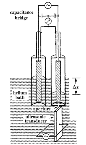
Figure 8: The Richards-Anderson cell (1965).

In order to observe the Josephson ac-effect in superfluid helium, Richards and Anderson (1965) designed an experiment based on the beat note expected to form between the sound wave emitted by a quartz transducer immersed in the superfluid and the internal pressure fluctuation due to the ac-effect. In this historical setup, shown in Fig.8, two identical coaxial capacitors are suspended over a liquid helium bath cooled at a temperature below the lambda point (of the order of 1.15 K). One of the capacitors is fully open-ended, the other is partially closed at the bottom by nickel foil with a very small aperture. The foil is 25 micrometres thick, in which a 15 micrometre aperture had been punched with a sharp needle: the pinhole thus manufactured constitutes the “weak link” between the two superfluid pools.

If a helium level difference $\Delta z$ between the two coaxial capacitors is created by lowering and raising the whole assembly over the liquid helium bath, the return to hydrostatic equilibrium is impeded by the pressure head of the steady stream of vortices corresponding to Eq.(38). The level difference can be precisely monitored by a capacitance bridge. When an ultrasound wave is shone by a quartz transducer facing the micro-aperture as shown in Fig.8, it can couple to the stream of vortices and modulate the flow.

Steps in the return to equilibrium were indeed observed at level differences which were multiples and submultiples of the fundamental head difference frequency expected from the Josephson ac relation: $\Delta z=n\,\hbar\omega\,/\,n^{\prime}\,m_{4}g\;$ where $n$ and $n^{\prime}$ are integers, and $g$ the acceleration of gravity. Richards and Anderson’s results were reproduced by other researchers using similar setups, notably Khorana and Chandrasekhar (1967), Khorana (1969), Hulin et al. (1971), and Hulin et al. (1972). Different setups, involving rotating or oscillating toroidal cells (Guernsey, 1971; Gregory, 1972), vortices accelerated by ions (Carey et al., 1973), a two-orifice flow arrangement (Gamota, 1974) were also tried but with mixed success at best, suffering from lack of reproducibility and poised with numerous unexpected features.

It eventually became clear that the early claims of observation of the Josephson ac effect by synchronisation of the pressure head on the sound frequency did not meet universal acceptance. On the contrary, an alternate explanation in terms of acoustic standing waves in the cell was put forward on experimental grounds by Leiderer and Pobell (1973), as well as Musinski and Douglass (1972) (Musinski, 1973), and on theoretical grounds by Rudnick (1973). It was nonetheless argued by Anderson and Richards (1975) that, although acoustic resonances in the cell could be a concern, they could not account for all of the features observed in their experiments.

These efforts directed toward the demonstration of the hydrodynamic Josephson effects, together with direct studies of the critical velocity itself (Trela and Fairbank, 1967; Gamota, 1973), did bring experimental confirmation of the views of Feynman and Anderson that vortices were associated with the appearance of dissipation in superfluid flow. However, quantitative studies leading to a clear picture of how these vortices were created and how they interacted with the superflow were lacking. A consensus grew that somehow their formation and evolution had a chaotic character, presumably due to random pre-existing vorticity in the superfluid and to a probable evolution toward some form of turbulent motion of the quantised vortices, a belief confirmed in part by the more recent studies described in Sec.VI. The flurry of activity stirred by the initial reports of observations related to the Josephson effects in helium receded almost completely.

With the hindsight gained from the experiments described further on, it can now be concluded that the synchronisation envisioned by Richards and Anderson (1965) would be nigh impossible to achieve. A particularly clear exposition of this synchronisation experiment is given by Anderson et al. (1984) in terms of parametric effects due to the system non-linearities, of the same kind as frequency pulling in radiofrequency oscillators. These effects require that energy be stored reversibly in a non-linear element, here the Josephson junction or, for rf-devices, a non-linear inductance. In ⁴He far from the l-point the relation between the current and the phase difference across the weak link shows no non-linearities. The energy that the vortices gather from the potential flow is carried swiftly away from the orifice and is irreversibly lost. It can be used to pull or push the flow in synchronism with the sound excitation for a very brief lapse of time only, much shorter than the period of the audiofrequencies used in these experiments. Furthermore, for the comparatively large orifices used then, vortices appear in a rather irregular fashion, not individually but in lumps with varying numbers, as discussed in Sec.VI.2. These peculiarities hamper the eventual synchronisation to a regular pattern of steps.

III.2 The hydromechanical resonator

In the early eighties, several groups went on striving to improve the detection techniques used in the search for the hydrodynamical Josephson effects. The use of a diaphragm-driven hydromechanical resonator fully immersed in the superfluid was pioneered by Zimmermann, Jr., and his students. A similar device with two chambers was built by Manninen and Pekola (1983) for critical velocity measurements in superfluid ³He, and used by Lounasmaa et al. (1983) for the search of an ac Josephson effect in superfluid ³He, a topic that will be covered in Sect. VII.2. The expertise developed at Cornell on torsional oscillators was put to use in superfluid ³He by Reppy and his students (Crooker, 1984). Again, the hydrodynamic Josephson effects could not be observed in these various experiments, for one or several of the following reasons:

• $\bullet$ the apertures used as weak links were too large;

• $\bullet$ the mass flow rate sensitivity was marginally adequate only;

• $\bullet$ the superfluid motion was driven from current sources that were too stiff to let the response of the weak link be seen;

• $\bullet$ and, last but not least, the cells were too bulky and too sensitive to external mechanical vibrations to allow for non-invasive measurements.

The first reason was clearly perceived as essential. Efforts shifted from superfluid ⁴He to the newly discovered superfluid ³He because the coherence length is two orders of magnitude larger, putting the fabrication of a genuinely-weak superfluid link within reach of experimental low temperature physicists. Work was carried out in that direction by Wirth and Zimmermann, Jr. (1981), who were the first to use sub-micronic orifices in free-standing ultra-thin foils, and others (Sudraud et al., 1987),(Amar et al., 1990).

The detection of the minute mass currents that would flow in micro-apertures improved markedly in the early eighties as reliable rf-SQUIDs became available. Ultra-sensitive pressure and displacement gauges could then be developed (Avenel and Varoquaux, 1986a).

III.3 Early phase slippage experiments

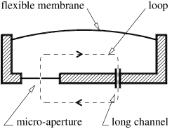
Figure 9: Schematic drawing of the flexible-diaphragm double-hole hydromechanical resonator. The dashed line shows a closed loop threading the two holes – micro-aperture and long channel – located entirely in the superfluid.

The phase slippage experiments that were carried out starting from the mid-eighties using these refined techniques Varoquaux et al. (1987); Avenel and Varoquaux (1985) confirmed Feynman and Anderson’s views on dissipation in superflows and brought a large measure of clarification to the critical velocity problem Varoquaux et al. (1991) and to the formation of vortices in superfluid ⁴He Avenel et al. (1993). These experimental results and their interpretation have since been largely confirmed by other workers.

The design of the first weak link in which hydrodynamical Josephson effects were seen (Sudraud et al., 1987) struck a compromise between to two conflicting requirements, that it be weak enough to effectively depress the wavefunction amplitude while preserving the macroscopic coherence of the superfluid, and that it be big enough to let a measurable flow of liquid go through. A slit geometry was chosen for the micro-aperture, the smaller dimension of which was comparable with the coherence length in superfluid ³He, $\xi_{0}$, which is in the sub-micron range (see §VII.2). This orifice was micro-machined by ion-milling in a free standing foil the thickness of which was also comparable to $\xi_{0}$. The third dimension of the slit was made large to provide a substantial cross sectional area through which the superfluid would flow.

Phase slippage was studied with the help of a miniature hydromechanical device, represented schematically in Fig.9, which is basically a flexible-wall Helmholtz resonator with two vents, immersed in the superfluid bath. The flexible wall is constituted by a Kapton membrane coated with aluminium. In the version shown in Fig.9, there are two openings connecting the resonator chamber to the main superfluid bath. One is a micro-aperture in which the critical velocity is reached. The critical event consists in a sudden change of the resonance amplitude corresponding to a departure from the expected classical hydrodynamics response of the flow velocity through the micro-aperture as discussed in the following. The other opening is a relatively open duct and provides a parallel path to the superfluid, along which the quantum phase remains well determined in all circumstances. The velocity circulation along the superfluid closed loop threading the two openings shown in Fig.9 changes by an integral number of quanta for each critical event.

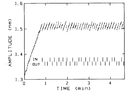
Figure 10: Time chart of the peak resonance amplitude of the resonator membrane, in nm, for positive and for negative excursions. Each dot represents a measurement. The time interval between individual measurements is half a period, 177 ms here. The ticks labelled “in” and “out” indicate whether the jumps occur when the liquid flows in or out of the cell. The drive power applied to drive the resonance is very small ($2.4\;10^{-18}$ W). When the peak amplitude is subcritical, its value builds up linearly with time as seen at the left of the chart. The critical events are sharply defined and quite reproducible but occur at a threshold that varies slightly from event to event. The superfluid ⁴He contained 100 to 300 ppb of ³He and was cooled to about 10 mK under a very small hydrostatic pressure head. From Avenel and Varoquaux (1985).

The operation of these resonators is described in detail in the literature. Flow is driven in and out of the resonator by an electrostatic ac-drive applied to the aluminium-coated Kapton membrane. The membrane is mounted in such way as to be as flexible as possible; it provides the restoring elastic force in the resonator. The “common mode” flow of liquid in and out of the cell body through the two vents of the resonator provides a force of inertia to the hydromechanical device. These inertial and elastic terms determine the resonance frequency. The device is usually driven at or close to resonance in continuous mode. The raw data consist of peak amplitude charts as represented in Fig.10. A strong impulsive force may also be applied to the membrane; the large transient response of the resonator reveals additional features when it becomes non-linear.

In the absence of dissipation, the resonance motion under a small steady ac drive increases linearly in amplitude under the action of the drive as energy gradually gets stored in the resonator. This linear rise on the left of the trace in Fig.10 proceeds until the flow velocity in the micro-aperture becomes critical. Sudden drops of the peak amplitude from one half-cycle to the next then appear. These drops signal that a lump of resonator energy has been lost between two successive recordings of the absolute peak amplitude. Quite importantly, these lumps are identical – to experimental uncertainty – from event to event.

These events are interpreted as the footprint left by vortices crossing the potential flow pattern in the vicinity of the micro-aperture. In their course, they cut all potential flow lines, pick up energy at the expense of the potential flow of the resonator and change the phase difference along these flow lines by $2\pi$. Hence the name “phase slips”. These slips of the phase are sudden and take place at a fairly well defined threshold, which defines the phase slip critical velocity. It will become apparent in the following that this critical velocity, while signalling a breakdown of superfluidity, differs from other quantities also called “critical velocities”. These features are discussed in detail further on, in Secs.V and V.5.

III.4 Phase-slippage experimental results

The observation of phase slips in ⁴He has led to a number of quite significant results. They brought a confirmation of Anderson’s ideas, much welcome in view of the controversies about previous experiments. And quite importantly, they have shed light on the previously indecipherable problems of the critical velocity and of vortex nucleation. Below are summarised their most important qualitative features and some of their implications.

1. The critical velocity threshold, which can be seen on time charts such as that shown in Fig.10, is markedly temperature-dependent down to below 200 mK and reaches a well-defined plateau below 150 mK. These features are shown in Fig.12 and are analysed in Sec.V below. As the thermodynamic properties of superfluid ⁴He are very nearly independent of temperature below 1 K, this observation indicates that the critical process in action is not governed solely by hydrodynamics. Statistical mechanics may well play the leading role.

2. Aperture size is not found to be a relevant factor, as long as it is “small enough”, roughly below a few mm. This feature and the temperature dependence mentioned above are in sharp contrast with the Feynman critical velocity, which, as discussed below in §IV.2, exhibits a well-characterised dependence on size and none on temperature (except very close to the l transition).

3. The actual velocity threshold for phase slips shows significant scatter from one slip to the next in a given sequence, as can be seen in Fig.23. This scatter lies much above the instrumental noise level of peak amplitude detection. It represents a genuine stochastic property of the physical process at work, which turns out to display a temperature dependence similar to that of the critical velocity itself, as shown in Fig.13.

4. The phase slip pattern shows quite reproducible properties in the course of a given cool-down as long as the experimental cell is kept at a temperature below 10$\sim$15 K. If the temperature is cycled up to liquid nitrogen temperature and down again, small changes to the critical threshold and to the pattern itself can occur. These changes reveal the importance of minute alterations in the surface state of the cell, e.g., contamination of the micro-aperture walls by solidified gases during thermal cycling.

5. Quite importantly, phase slips are the signature that quantised vortices are created in aperture flow above a well-defined threshold of flow velocity. This statement is based on the measured value of the phase change, found to be $2\pi$ to the accuracy of the experiment (Avenel and Varoquaux, 1985). This amounts to a change of precisely one quantum of circulation in the superfluid loop threading the micro-aperture and the long parallel channel. A detailed scenario for the occurrence and development of these phase slips has been described by Burkhart et al. (1994) and is discussed below in Sec.V.5.

Critical velocities and phase slips in the superfluid phases of ³He show different features that will be briefly touched upon in Sect.VI.

IV Critical velocities in superfluids

The critical velocity in a superfluid is defined as the threshold above which the flow of the superfluid component becomes dissipative, that is, the property of superfluidity is lost. This rather broad definition encompasses a number of different physical situations. This Section begins with an overview of the different brands of “critical” velocities that comply with this definition. It will end up by focusing on that which involves the phase slip phenomenon, namely, the nucleation of superfluid vortices.

Neither the problem of critical velocities in superfluids nor that of the nucleation of vortices are new. The former is as old as the discovery of superfluidity (see the monograph by Wilks (1967)). The latter, first discussed by Vinen in the early sixties Vinen (1963), has met an even more tortuous fate. It was first thought, still was in some quarters not so long ago, to be nigh impossible: such an extended hydrodynamical object as a vortex line with a finite circulation involving the collective motion of a large number of helium atoms would have a vanishingly small probability of occurring spontaneously. More recent experiments probing superflow on a finer scale of length have shown otherwise.

IV.1 The Landau criterion

As discussed previously in §I.1, Landau (1941) explained the absence of dissipation in the flow of helium-4 by the existence of a sharply defined dispersion curve for elementary excitations, the phonons and the rotons. This property is now associated with the phenomenon of Bose-Einstein condensation (Griffin, 1987, 1993), as has long been suspected (London, 1954). Elementary excitation energy levels $\epsilon(\mathbf{p})$ are well defined. They have a negligible spread in energy. States with very low energy are thus extremely rare. This scarcity of low-lying states is held responsible for the inviscid property of ⁴He.

An impurity, or a solid obstacle, can only exchange an energy $\epsilon(\mathbf{p})$ at momentum $\mathbf{p}$ that exactly matches the energy of an elementary excitation of the fluid. If the superfluid moves at velocity $\mathbf{v}_{\mathrm{s}}$, the energy of elementary excitations in the frame of reference at rest becomes $\epsilon-\mathbf{v}_{\mathrm{s}}\cdot\mathbf{p}$ Wilks (1967); Baym (1969). The same holds for a moving obstacle, by Galilean invariance. If this energy turns negative, elementary excitations proliferate and superfluidity is lost. The condition on the superfluid velocity for this to happen reads:

$$v_{\mathrm{s}}\geqslant v_{\mathrm{L}}=\frac{\epsilon(p)}{p}\Big{|}_{\mathrm{min}}\simeq\frac{\epsilon(p)}{p}\Big{|}_{\mathrm{roton}}\;.$$ (44)

Unless this condition is met, there is no dissipative interaction between the fluid and its surroundings: the flow is viscousless.

The minimum value of $\epsilon/p$ for helium lies very close to the roton minimum, as shown in Fig.1. This means that rotons are created when the Landau critical velocity is reached in ⁴He. At low pressure, the roton minimum parameters are such that $v_{\mathrm{L}}\simeq 60$ m/s. The Landau critical velocity has been observed under certain conditions in the propagation of ions in which rotons are created in ⁴He as reviewed by McClintock and Bowley (1995). The much less dense Bose-Einstein Condensed gases sustain a phonon-like energy spectrum at low momentum (Bogolyubov, 1947) and no roton-like features; the Landau velocity is the sound velocity, $c=\epsilon(p)/p|_{p=0}$ and phonons are emitted. The Landau critical velocity $v_{\mathrm{L}}$ in superfluid ⁴He is smaller than the sound velocity ($c=220$ m/s at low pressure) but is still quite larger than the critical velocities observed in most experiments.

IV.2 Feynman’s approach

Feynman (1955) realised, following Onsager, that not only would vorticity be quantised in ⁴He in units of the quantum of circulation $\kappa_{4}=2\pi\hbar/m_{4}$  but, preceding Anderson, that these vortices would be responsible for the onset of dissipation and for a critical velocity in the superfluid. In Feynman’s views, vortices would be puffed out of the mouth of orifices much in the way of smoke rings – or von Karmann alleys past obstacles in classical (Navier-Stokes) fluids.

Such vortex rings can be treated as elementary excitations of the superfluid, which they rightfully are from the vantage point taken in Sec.II. Hence Landau’s criterion applies. The limiting velocity associated with these vortex rings, assumed to be circular, can be evaluated from the expressions for the energy $E_{\mathrm{R}}$ and impulse $P_{\mathrm{R}}$, Eqs.(24) and (32). The critical value set by Eq.(44) is reached for a radius $R$ such that $E_{\mathrm{R}}/P_{\mathrm{R}}$ is at a minimum, which occurs when $R$ is as large as feasible, that is, of the order of the orifice size $d$. This minimum value sets the lowest velocity at which vortices can start to appear and defines the Feynman critical velocity:

$$v_{\mathrm{F}}\simeq\frac{\kappa_{4}}{2\pi d}\ln\left(\frac{d}{a_{0}}\right)\;.$$ (45)

As discussed below, $v_{\mathrm{F}}$ is much closer to experimental values than the Landau critical velocity for rotons. Although this agreement is heartening, it also raises questions: how do these vortices come about and how do they evolve?

IV.3 Several kinds of critical velocities

The compilation of the critical velocity data in various apertures and channels from various sources available at the time of the Exeter Meeting in 1990 Varoquaux et al. (1991) is shown in Fig.11 together with more recent data. Two different critical velocity regimes appear clearly on this graph, a fast regime for small apertures, of the phase-slip type, which is temperature-dependent, and a slower regime for larger channels, of the Feynman type, which is temperature-independent. The data points from various sources for these two different types of critical velocity do not fall on well-defined lines but merely bunch into clusters of points. As already stated, critical velocities in apertures and capillaries are not very reproducible from experiment to experiment indicating that, besides size, temperature, and pressure, some less-well-controlled parameters also exert an influence. In some occasions, switching between these two types of critical velocity has been observed in the course of the same cool-down Hulin et al. (1974); Zimmermann, Jr. (1993a).

The critical velocity that depends on channel size does follow on average relation (45) for the Feynman mechanism. The higher critical velocities, bunched around 5 to 10 m/s, faster than the Feynman $v_{\mathrm{F}}$ even for the smallest apertures but still considerably slower than Landau’s $v_{\mathrm{L}}$ relate to the phase slip phenomenon and are discussed below.

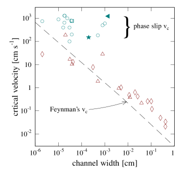
Figure 11: (Color online) Critical velocity data vs channel width ($\diamond$) – Wilks (1967); ($\circ$) and ($\scriptstyle\triangle$) – temperature-dependent and temperature-independent data as compiled byVaroquaux et al. (1991); ($\blacktriangleleft$) – Shifflett and Hess (1995); ($\star$) – Flaten et al. (2006b); ($\square$) – Steinhauer et al. (1995) as reanalysed by Varoquaux and Avenel (1996a). For the temperature-dependent data, the highest value, i.e., that at the lowest temperature, has been retained. The dashed line is obtained from Eq.(45) for the Feynman critical velocity.

As a basis for comparison, it is worthwhile to summarise the findings of the ion propagation studies in superfluid ⁴He at various pressures, which have been reviewed by McClintock and Bowley (1991, 1995). Ions can be created in liquid helium and accelerated by electric field until they reach a limiting velocity. The resulting drift velocities are measured by time-of-flight techniques. For negative ions, hollow bubbles 30 Å in diameter with an electron inside, two different behaviours are observed:

• Below about 10 bars, vortex rings are created, on the core of which single electrons get trapped: the drift velocity suddenly drops from that of the negatively charged bubbles to that of the much slower vortex rings (Rayfield and Reif, 1964).

• Above 10 bars, the accelerated ion runs into the roton emission mechanism before vortex rings can be created. The Landau critical velocity is observed to be $\approx$ 46 m/s at 24 bars down from a calculated value of 60 m/s at SVT as the roton parameters change with pressure while the vortex creation velocity increases with pressure (Varoquaux and Avenel, 1996b).

• Around 10 bars, both critical velocities, the Landau critical velocity for the formation of rotons and that for the formation of vortex rings can be observed to occur simultaneously because ions can be accelerated above the threshold for roton emission.

These ion propagation measurements provide a vivid illustration not only of the existence of a critical velocity obeying the Landau criterion but also that roton creation and vortex formation constitute different phenomena and can exist concurrently. The vortex emission threshold displays other noteworthy features. It depends on temperature in a non-trivial way, comparable to that of the phase-slip and also shows the marked dependence on ³He impurity concentration observed for phase slips in micro-aperture flows but not in larger channels. In both ion propagation and aperture flow measurements, vortex formation displays similar features.

Altogether, a study of the experimental data in superfluid ⁴He reveals three different, well-defined, types of critical velocities; one, the celebrated Landau critical velocity, $v_{\mathrm{L}}$, observed in ⁴He only for ion propagation; another, $v_{\mathrm{F}}$, that appears to follow the Feynman criterion as shown in Fig.11 with all the uncertainties on the hydrodynamical process of vortex creation in larger channels; and a third, $v_{\mathrm{c}}$, for phase slips, in want of an explanation: how are the vortices of phase slips in aperture flow created, and how does the situation differ from that in larger channels?

The short answer, based on qualitative evidence, is that the temperature dependence of $v_{\mathrm{c}}$ and its stochastic properties clearly point toward a process of nucleation by thermal activation above $\sim$150 mK or so and by quantum tunnelling below. This conclusion contradicts the common-place daily observations of the formation of whirlpools and eddies, and also the widely held belief that large scale topological defects with a quantum charge of circulation cannot appear out of nowhere in the superfluid. It will be seen to hold in ⁴He only because the nucleated vortices have nanometric size, a fact that came to be appreciated because of the detailed analysis of phase slippage observations related below.

V Phase slip critical velocity: a stochastic process

A more firmly established answer to the question formulated above comes from a quantitative analysis of the experimental data for phase slips. The clues given below conclusively show that, in small apertures, vortices are nucleated by thermal activation above about 150 mK, and by quantum tunnelling below.

The first piece of evidence for the nucleation of vortices, that is their creation ex nihilo, rests on the temperature dependence of the phase-slip critical velocity shown in Fig.12. This figure, as Fig.11 (and Fig.13 to be discussed further on), represents an attempt to compare data from different groups. The data points are scattered but a general trend emerges. The phase slip critical velocity increases in a near-linear manner when the temperature decreases from 2 K to $\sim\,$0.2 K. That is, the functional dependence of $v_{\mathrm{c}}$ upon $T$ goes as $v_{\mathrm{c}}=v_{0}(1-T/T_{0})$. The data depart from this linear dependence below 200 mK, where they reach a plateau, and above 2 K because the critical velocity goes to zero at $T_{\mbox{\footnotesize{l}}}$.

This temperature dependence, first observed in 1985 at Orsay (Varoquaux et al., 1987, 2001) and now a well-established experimental fact (Zimmermann, Jr. et al., 1998), (Steinhauer et al., 1995) is very telling. It came as a surprise at first because the critical velocities observed before were temperature-independent below $\sim$1 K. As the quantum fluid is nearly fully in its ground state below 1 K – the normal fluid fraction becomes less than 1 % – one is led to suspect that a Arrhenius-type process must come into play. If such is the case, that is, if thermal fluctuations in the fluid with an energy of at most a few $k_{\mathrm{B}}T$ can trigger the appearance of fully-formed vortex out of nowhere, the energy of this vortex must also be of the order of a few $k_{\mathrm{B}}T$: it must be a very small vortex. But very small vortices require rather large superfluid velocities to sustain themselves – as seen on Eq.(34). That these requirements can be met emerges from a detailed quantitative analysis of the experimental data in the framework of nucleation process.

The nucleation rate for a thermally activated process is expressed by Arrhenius’s  law:

$${\mathit{\Gamma}}_{\mathrm{K}}=\frac{\omega_{0}}{2\pi}\,\left[(1+\alpha^{2})^{1/2}-\alpha\right]\exp\left\{-\frac{E_{\mathrm{a}}}{k_{\mathrm{B}}T}\right\}\;.$$ (46)

where $\omega_{0}/2\pi$ is the attempt frequency and $E_{\mathrm{a}}$ the activation energy of the process, which depends on the velocity $v_{\mathrm{p}}$ and, more weakly, on the pressure $P$ and the temperature $T$. The correction for dissipation in the square brackets has been introduced by Kramers (1940) to describe the escape of a particle trapped in a potential well and interacting with a thermal bath in its environment. The particle undergoes Brownian motion fluctuations and experiences dissipation. This dissipation is characterised by a dimensionless coefficient $\alpha=1/(2\omega_{0}\tau)$, $\tau$ being the time of relaxation of the system toward equilibrium. In superfluid helium, dissipation is small. Although some dissipation is necessary for the system to reach equilibrium with its environment, its influence on the thermal activation rate is very small and will be neglected in the following. However, this will not be anymore so in the quantum regime, considered below, because dissipation causes decoherence.

The expression for the critical velocity that stems from the Arrhenius rate, Eq.(46), is derived as follows. In experiments such as those shown in Fig.10, the velocity varies periodically at the resonance frequency as $v_{\mathrm{p}}\,\cos(\omega t)$, $v_{\mathrm{p}}$ being the peak velocity of the potential flow. The probability that a phase slip takes place during the half-cycle $\omega t_{\mathrm{i}}=-\pi/2\,,\;\omega t_{\mathrm{f}}=\pi/2$ is

$$p = 1-\exp\left\{-\int_{t_{\mathrm{i}}}^{t_{\mathrm{f}}}\mathit{\Gamma}_{\mathrm{K}}(P,T,v_{\mathrm{p}}\cos(\omega t^{\prime})\right\}dt^{\prime}$$

$$= 1-\exp\left\{-\frac{\omega_{0}}{2\pi\omega}\sqrt{\frac{-2\pi k_{\mathrm{B}}T}{v_{\mathrm{p}}\left.\left.\partial{E_{\mathrm{a}}}\right/\partial{v}\right|_{\mathrm{t}=0}}}\exp\left\{-\frac{E_{\mathrm{a}}}{k_{\mathrm{B}}T}\right\}\right\}.$$

The last equation (V) results from an asymptotic evaluation of the integral at the saddle point $t=0$.

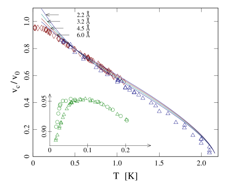
Figure 12: (Color online) Critical velocity, normalised to the zero temperature linear extrapolation value $v_{0}$, vs $T$, in kelvin: ($\diamond$), Avenel et al. (1993), for ultra-pure ⁴He; ($\scriptstyle\triangle$), Zimmermann, Jr. et al. (1998). The plain curves are computed from the half-ring model (see §V.5) for $a_{0}$ = 2.2, 3.2, 4.5, 6.0 Å and are normalised to match the experimental value at 0.5 K. The inset shows the influence of ³He impurities on $v_{\mathrm{c}}$: ($\circ$), 3 ppb ³He in ⁴He; ($\scriptstyle\triangle$), 45 ppb, from Varoquaux et al. (1993). Adapted from (Varoquaux et al., 2001).

The critical velocity $v_{\mathrm{c}}$ is defined as the velocity for which $p=1/2$. This definition is independent of the experimental setup, except for the occurrence in Eq.(V) of the natural frequency of the hydromechanical resonator $\omega$. The implicit relation between $v_{\mathrm{c}}$ and $E_{\mathrm{a}}$ then reads:

$$\frac{\omega_{0}}{2\pi\omega}\sqrt{\frac{-2\pi k_{\mathrm{B}}T}{v_{\mathrm{c}}\left.\left.\partial{E_{\mathrm{a}}}\right/\partial{v}\right|_{v_{\mathrm{c}}}}}\exp\left\{-\frac{E_{\mathrm{a}}(P,T,v_{\mathrm{c}})}{k_{\mathrm{B}}T}\right\}=\ln 2\;.$$ (48)

In Eq.(48), the attempt frequency is normalised by the resonator drive frequency: the Brownian particle attempts to escape from the potential well at rate $\omega_{0}/2\pi$ but an escape event is likely only in the time window in a given half-cycle of the resonance during which the energy barrier stays close to its minimum value $E_{\mathrm{a}}(v_{\mathrm{c}})$. This time interval is inversely proportional to $\omega$, which explains why an instrumental parameter gets its way into Eqs.(V) and (48).

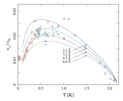
Figure 13: (Color online) Statistical width of the critical velocity transition, normalised to the linear extrapolation limit at $T=0$, $v_{0}$, in terms of temperature: ($\diamond$), Avenel et al. (1993); ($\scriptstyle\triangle$), Zimmermann, Jr. et al. (1998); ($\times$), Steinhauer et al. (1995). The plain curves are computed as in Fig.12 for four values for $a_{0}$. Adapted from Varoquaux et al. (2001).

The velocity at which each individual critical event takes place is a stochastic quantity. Its statistical spread can be characterised by the ​̀​̀width” of the probability distribution defined Avenel et al. (1993); Zimmermann, Jr. et al. (1990) as the inverse of the slope of the distribution at $v_{\mathrm{c}}$, $\left({\partial p/\partial v|_{v_{\mathrm{c}}}}\right)^{-1}$. This critical width is found to be expressed by:

$$\Delta v_{\mathrm{c}}=-\frac{2}{\ln 2}\left[\frac{1}{2}\left\{\frac{1}{v_{\mathrm{c}}}+\left.\left.\frac{\partial^{2}E_{\mathrm{a}}}{\partial v^{2}}\right|_{v_{\mathrm{c}}}\right/\left.\frac{\partial E_{\mathrm{a}}}{\partial v}\right|_{v_{\mathrm{c}}}\right\}+\frac{1}{k_{\mathrm{B}}T}\left.\frac{\partial E_{\mathrm{a}}}{\partial v}\right|_{v_{\mathrm{c}}}\right]^{-1}\;.$$ (49)

The quantities $v_{\mathrm{c}}$ and $\Delta v_{\mathrm{c}}$ are derived from $p$, itself obtained by integrating the histograms of the number of nucleation events ordered in velocity bins. The outcome of this procedure is illustrated in Fig. 14: $p$ shows an asymmetric-S shape characteristic of the double exponential dependence of $p$ on $v$, Eq.(V), a consequence of Arrhenius’s  law, Eq.(46), being plugged into a Poisson probability distribution. The observation of this asymmetric-S probability distribution constitutes an additional experimental clue for the existence of a nucleation process. The quantities $v_{\mathrm{c}}$ and $\Delta v_{\mathrm{c}}$ are easily extracted from the probability curves $p(v)$, but the inverse path from $v_{\mathrm{c}}$ and $\Delta v_{\mathrm{c}}$ back to $E_{\mathrm{a}}(v)$ and $\omega_{0}$ by numerical integration of the differential equation (48) leads to inaccurate results.

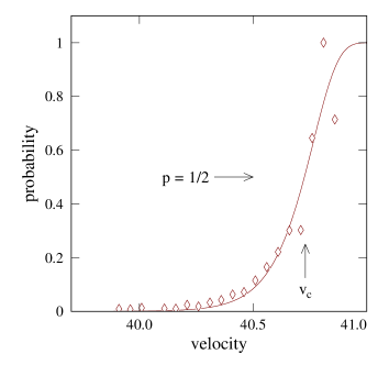
Figure 14: (Color online) Probability $p$ vs phase slip velocity in winding number. The plain curve is a non-linear least square fit to the analytic form Eq.(V), which contains two adjustable parameters, $v_{\mathrm{c}}$ and $\Delta v_{\mathrm{c}}$. The critical velocity resulting from this distribution of the measured values is defined as the fit value for $p=1/2$. The critical velocity distribution width is given by the slope at $p=1/2$. From Varoquaux and Avenel (2003).

In view of these difficulties Varoquaux and Avenel (2003) improved the data analysis by obtaining the escape rate $\mathit{\Gamma}(v)$ directly from the phase slip data. This rate is the ratio in any velocity bin of the number of slips that have occurred at that velocity to the total time spent by the system at that given velocity. The outcome of this procedure is illustrated in Fig. 15. The slope of $\ln\mathit{\Gamma}(v)$ directly yields $\left.{\partial E_{\mathrm{a}}/\partial v}\right|_{v_{\mathrm{c}}}$; the value of $\ln\mathit{\Gamma}$ at $v_{\mathrm{c}}$ gives a combination of $\ln\omega_{0}$ and $E_{\mathrm{a}}(v_{\mathrm{c}})$.

The need to solve Eq.(48) has been alleviated but to cleanly disentangle these two quantities and solve this inverse problem is still error prone. At this point experiment itself offers help as will shortly be shown.

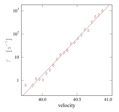
Figure 15: Nucleation rate $\mathit{\Gamma}$ expressed in s^-1 on a semi-logarithmic scale vs slip velocity in winding number in ultra-pure ⁴He at 17.70 mK and saturated vapour pressure. The line is a linear fit to the data. From Varoquaux and Avenel (2003).

V.1 Vortex nucleation: thermal vs quantum

Below $\sim$ 0.15 K, the phase slip critical velocity $v_{\mathrm{c}}$ suddenly ceases to vary with $T$, as seen in Fig. 12 for ultra-pure ⁴He, $v_{\mathrm{c}}(T)$ remains flat down to the lowest temperatures ($\sim\,$12 mK). The effect of ³He impurities, shown in the inset, could mimic the appearance of such a plateau but is ruled out because of the extreme purity of the ⁴He sample, which contains less than 1 part in 10⁹ of ³He impurities. The crossover between these two regimes is very sharp. At the same crossover temperature $T_{\mathrm{q}}$, $\Delta v_{\mathrm{c}}$ also levels off sharply. It is believed on experimental grounds that this saturation is intrinsic and is not due to stray heating or parasitic mechanical vibrations Avenel et al. (1993).

If the nucleation barrier were undergoing an abrupt change at $T_{\mathrm{q}}$, for instance because of a bifurcation toward a vortex instability of a different nature Josserand and Pomeau (1995), in all likelihood $\Delta v_{\mathrm{c}}$ would jump to a different value characteristic of the new process (presumably small since $v_{\mathrm{c}}$ reaches a plateau). Such a jump is not observed in Fig. 13. Furthermore, $v_{\mathrm{c}}$ levels off below $T_{\mathrm{q}}$, which would imply through Eq.(48) that $E_{a}$ becomes a very steep function of $v$, but $\Delta v_{\mathrm{c}}$ also levels off, which, through Eq.(49), would imply the contrary. This discussion leads one to investigate the possibility that, below $T_{\mathrm{q}}$, thermally-assisted escape over the barrier gives way to quantum tunnelling under the barrier Ihas et al. (1992). This switch from thermal to quantum does induce plateaus below $T_{\mathrm{q}}$ for both $v_{\mathrm{c}}$ and $\Delta v_{\mathrm{c}}$.

Independently of these phase slippage studies, the group of Peter McClintock at Lancaster had also reached the conclusion from their ion propagation experiments of the existence of a crossover around 300 mK from a thermal to a quantum regime for the nucleation of vortices Hendry et al. (1988), as predicted by Muirhead, Vinen, and Donnelly Muirhead et al. (1984). There certainly are significant differences between the ion limiting drift velocity and aperture critical flow – in particular, the latter is nearly one order of magnitude smaller – but the qualitative similarities are strikingly telling. The two completely different types of experiments indicate that vortices would appear as a result of a nucleation process on a nanometric scale, both in a thermal regime above $T_{\mathrm{q}}$ and in a quantum one below.

V.2 The macroscopic quantum tunnelling rate

Taking this hint at face value, zero point fluctuations are now assumed to overtake thermal fluctuations below $T_{\mathrm{q}}$: the potential barrier is not surmounted with the assistance of a large thermal fluctuation, it is tunnelled under quantum-mechanically; the quantum-tunnelling event is “assisted” by the zero point fluctuations, so to speak Martinis and Grabert (1988), in the same manner as the Arrhenius process is assisted by thermal fluctuations. What is remarkable here, and not so easy to admit at first, is that such a tunnelling process affects a macroscopic number of atoms, those necessary to form a vortex of about 50 Å in length, as turns out to be the case.

These “macroscopic quantum tunnelling” (MQT) processes have been the object of numerous experimental and theoretical studies, mainly in superconducting Josephson devices Caldeira and Leggett (1983) . The case for vortices in helium can be worked out in a similar manner.

The quantum tunnelling rate of escape of a particle out of a potential well $V(q)$ is a textbook problem. The rate is proportional to $\exp{-S/\hbar}$, $S$ being, in the WKB approximation, the action of the escaping particle along the saddle-point trajectory at the top of the potential barrier, the so-called “bounce” Coleman (1977). For a particle of mass $m$ and energy $E$ escaping from a one-dimensional barrier $V(q)$, this action reads

$$S=2\int_{q_{1}}^{q_{2}}\mathrm{d}q\sqrt{2m[V(q)-E]}\;.$$ (50)

The determination of the bounce yields the generalised coordinates $q_{1}$ and $q_{2}$ of the points at which the particle enters and leaves the barrier. A discussion of the quantum tunnelling of vortices in terms of Eq.(50) thus requires a Lagrangian formulation of vortex dynamics. Such a formulation has been carried out in particular by Sonin (1995) and by Fischer (2000). However, analytic results can be obtained only at the cost of approximations that yield a less than fair comparison with experiments as discussed by Varoquaux et al. (2001).

A simplified and more productive approach can be borrowed from the literature for Josephson devices. Extending the work of Caldeira and Leggett (1983), and Larkin et al. (1984) to vortices in helium, Varoquaux (2006) has used for $V(q)$ a simple analytic form reduced to a sum of two terms, respectively parabolic and cubic in $q$:

$$V(q)=V_{0}+\frac{1}{2}m\omega_{0}^{2}q^{2}\big{(}1-\frac{2q}{3q_{\mathrm{b}}}\big{)}\;,$$ (51)

where $\omega_{0}$ is the angular frequency of the lowest mode of the trapped particle (that will be found comparable to the attempt frequency) and $q_{\mathrm{b}}$ the generalised coordinate of the barrier top location. The barrier height $E_{\mathrm{b}}$ is expressed in terms of these two parameters by $m\omega_{0}^{2}q_{\mathrm{b}}^{2}/6$.

Equation (51) expresses the vanishing potential barrier height when the applied velocity reaches the limiting velocity, $v_{\mathrm{c}0}$ at which the system “runs away”, the so-called “lability” point. At this point where the system becomes labile, the critical velocity is reached even in the absence of thermal or quantum fluctuations. Such a hydrodynamic instability threshold at which vortices appear spontaneously has been shown to occur in numerical simulations of flows past an obstacle using the Gross-Pitaevskii equation by Frisch et al. (1992) and others.

The zero-temperature WKB tunnelling rate for the phenomenological cubic-plus-parabolic potential $E_{\mathrm{b}}$, Eq.(51), is found to be Caldeira and Leggett (1983)

$$\mathit{\Gamma}_{0}=\frac{\omega_{0}}{2\pi}\,\left(120\pi\,\frac{S_{0}}{\hbar}\right)^{1/2}\exp-\frac{S_{0}}{\hbar}\;,$$ (52)

the action $S_{0}$ being equal to $36E_{\mathrm{b}}/5\omega_{0}$.

From this result, it can be anticipated that the crossover between the quantum and the thermal regime lies around a temperature close to that for which the exponents in Eqs.(46) and (52) are equal, namely $T=5\omega_{0}/36k_{\mathrm{B}}$ – assuming that the activation energy in Eq.(46), $E_{\mathrm{a}}$, reduces to the simple cubic-plus-parabolic form, $E_{\mathrm{b}}$. A more precise study of the mathematical properties of the quantum channel for escape leads to the following relation Mel’nikov (1991)

$$\hbar\omega_{0}=2\pi k_{B}T_{\mathrm{q}}\;.$$ (53)

Thus, from the experimental knowledge of the temperature of the crossover from thermal to quantal, $\omega_{0}$ is fixed to pinpoint accuracy by Eq.(53). Its value agrees with that (less precisely determined) obtained from the analysis of the Arrhenius regime outlined in the previous paragraph: some degree of self-consistency has been achieved. The values of the barrier height $E_{\mathrm{b}}$ at each given velocity then follow easily, using the full expressions for the rate in terms in terms of $E_{\mathrm{b}}$, $\omega_{0}$ and, also, for the damping parameter $\alpha$ as discussed below.

V.3 Friction in MQT

Damping turns out to matter significantly for quantum tunnelling of semi-macroscopic objects, contrarily to the thermal regime. The relevance and applicability of the concept of quantum tunnelling to macroscopic quantities such as the electric current through a Josephson junction or the flow of superfluid through a micro-aperture, although still sometimes questioned, have been checked in detail for the electrodynamic Josephson effect (Martinis et al., 1987). One of the conceptual problems is that, when a macroscopic quantum system is coupled to an environment that acts as a thermal bath, the coupling gives rise to a source of classical fluctuations and friction. The quantum process suffers decoherence and is profoundly affected.

This issue was tackled by Caldeira and Leggett Caldeira and Leggett (1983), and a number of other authors. For weak frequency-independent damping ($\alpha\ll 1$) and the cubic-plus-parabolic potential, the tunnelling rate takes the form:

$$\begin{split}{\mathit{\Gamma}}_{\mathrm{qt}}=&\frac{\omega_{0}}{2\pi}\,\left(864\pi\,\frac{E_{\mathrm{b}}}{\hbar\omega_{0}}\right)^{1/2}\times\exp\left\{-\,\frac{36}{5}\,\frac{E_{\mathrm{b}}}{\hbar\omega_{0}}\left[1+\frac{45\zeta(3)}{\pi^{3}}\alpha\right]\right.\\ &\left.+\frac{18}{\pi}\alpha\,\frac{T^{2}}{T_{\mathrm{q}}^{2}}+{\mathcal{O}}\left(\alpha^{2},\,\alpha\,\frac{T^{4}}{T_{\mathrm{q}}^{4}}\right)\right\}\;.\end{split}$$ (54)

According to Eq.(54), damping depresses the MQT escape rate at $T=0$ – $\alpha$ being a positive quantity – and introduces a temperature dependence that increases the rate as $T$ increases. These effects are large, even for weak damping, because they enter the exponent of the exponential factor in Eq.(54). Relation (53) between $T_{\mathrm{q}}$ and $\omega_{0}$ is nearly unaffected by damping: $\omega_{0}$ is simply changed into $\omega_{0}[(1+\alpha^{2})^{1/2}-\alpha]$ according to Eq.(46), a minor modification for $\alpha\ll 1$.

Figure 16: Potential well trapping a particle in one dimension. The particle can escape to the continuum of states to the right. The lowest mode at the bottom of the well has angular frequency $\omega_{0}$; $\omega_{\mathrm{b}}$ would be the corresponding quantity if the potential was inverted bottom over top. For the simple case of Eq.(51), $\omega_{0}=\omega_{\mathrm{b}}$. There can exist intermediate energy levels within the well, which are populated according to the Boltzmann factor. Particle escape can take place by quantum tunnelling “under” the barrier or by thermal activation “over” the barrier. The intermediate energy levels can be used as ladder rungs by the particle attempting to escape. These processes are embedded in Eq.(55).

Equation (54) is valid up to about $T_{\mathrm{q}}/2$. From $T_{\mathrm{q}}/2$ to $\sim T_{\mathrm{q}}$, one has to resort to numerical calculations Grabert et al. (1987). In the thermal activation regime, $T\gtrsim T_{\mathrm{q}}$, quantum corrections affect the Kramers escape rate up to about $3\,T_{\mathrm{q}}$ and can be evaluated analytically. These high-temperature quantum corrections depend only weakly on friction. A complete solution of the problem of the influence of friction, weak, moderate or strong, has first been worked out in the classical regime ($T\gg T_{\mathrm{q}}$) by Grabert (1988) and extended to the temperature range $T\gtrsim T_{\mathrm{q}}$ by Rips and Pollak (1989) who showed that the rate for arbitrary damping can be factorised in three terms,

$${\mathit{\Gamma}}=\,f_{\mathrm{q}}\,{\mathit{\Upsilon}}\,\mathit{\Gamma}_{\mathrm{K}}\;,$$ (55)

each term having a well-defined physical meaning: ${\mathit{\Gamma}}_{\mathrm{K}}$ is the classical Kramers rate, $f_{\mathrm{q}}$ the quantum correction factor, and $\mathit{\Upsilon}$ the depopulation factor. The high temperature limit of $f_{\mathrm{q}}$ is

$$f_{\mathrm{q}}=\exp\left\{\frac{\hbar^{2}}{24}\frac{(\omega_{0}^{2}+\omega_{\mathrm{b}}^{2})}{(k_{\mathrm{B}}T)^{2}}+{\mathcal{O}}(\alpha/T^{3},1/T^{4})\right\}\;,$$ (56)

in which $\omega_{0}$ and $\omega_{\mathrm{b}}$ are the confining potential parameters depicted in Fig.16. Analytic results for $f_{\mathrm{q}}$ are known to slightly below $T_{\mathrm{q}}$ Grabert et al. (1987); Hänggi et al. (1990).

The depopulation factor $\mathit{\Upsilon}$ arises from the depletion of the occupancy of the energy levels inside the potential well in the course of the escape process. This depletion occurs when the intermediate levels, if they exist, are not replenished fast enough by the thermal fluctuations. For the nucleation of vortices, friction turns out to always be both sufficient and not too large so that depopulation corrections remain small and $\mathit{\Upsilon}\sim 1$.

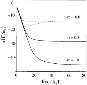
Figure 17: Logarithm of the escape rate normalised to the attempt frequency in terms of inverse temperature, also normalised to $\omega_{0}$ for various values of the damping parameter $\alpha$ (Grabert et al., 1987). The dotted line is a hand-sketch of the situation where $\alpha$ increases with temperature, starting from zero at $T=0$ (see §V.3). From Varoquaux and Avenel (2003).

The escape rate can be calculated over the full temperature range by piecing together Eqs.(46), (54), (55) and (56). The results for three values of the damping parameter $\alpha$ are shown in Fig.17. A hand-sketched line pictures the escape rate for $\alpha$ varying from zero at $T=0$ to 0.5 above $T_{\mathrm{q}}$: it is seen to actually decrease when the temperature increases from absolute zero. This unique situation is found in the nucleation of vortices in ⁴He as will now be described.

V.4 Experimental energy barrier and damping coefficient

The knowledge of the rate $\mathit{\Gamma}$ makes it possible to extract from the measured nucleation rate and crossover temperature the values of the energy barrier in terms of $v_{\mathrm{c}}$. The value of $\omega_{0}$ given by Eq.(53) ($\omega_{0}/2\pi=2\times 10^{10}$ Hz for $T_{q}$=0.147 K) is consistent with the attempt frequency appropriate to the thermally-activated regime Varoquaux et al. (1986) and that found directly from the fits to the probability $p$ as shown in Fig. 14. This agreement has been mentioned above.

This value of $\omega_{0}$ is comparable to the highest Kelvin mode eigenfrequency that a vortex filament in ⁴He can sustain. The Kelvin modes are helical waves with a dispersion relation expressed for a straight isolated vortex by

$$\omega^{\textstyle{\pm}}=\frac{\kappa_{4}}{\pi\,a_{0}^{2}}\left[1\pm\left\{1+ka_{0}\left[\frac{\mbox{K}_{0}(ka_{0})}{\mbox{K}_{1}(ka_{0})}\right]\right\}^{\frac{1}{2}}\right]\;,$$ (57)

where $\mbox{K}_{0}$ and $\mbox{K}_{1}$ are the modified Bessel functions of zeroth and first orders. In the short wavelength limit, $k^{-1}\rightarrow 0$, the high frequency mode reduces to:

$$\omega^{\textstyle{+}}=\frac{\kappa_{4}}{\pi a_{0}^{2}}\;.$$ (58)

Equation (58) sets the shortest time scale on which vortices can be expected to respond.

By analogy with the 2D-motion of point electric charges subjected to a rf magnetic field Muirhead et al. (1985), this frequency is sometimes called the “cyclotron” frequency. This frequency is that of the cycloidal motion taken by a long hollow cylinder impulsively pulled sideways in an inviscid fluid (Donnelly, 1991). The cylinder stands for the vortex core, assumed to be hollow and with radius $a_{0}$. The displaced mass per unit length of such a cylinder is $\rho\pi a_{0}^{2}$. For high frequency motions, the vortex mass is modified as discussed in §II.2.3, and Eq.(58) is renormalised to $\omega^{+}=\kappa_{4}/[\pi a_{0}^{2}{\mathrm{ln}}(r_{\mathrm{m}}/a_{0})]$, $r_{\mathrm{m}}$ being defined below Eq.(25). With $a_{0}=2.5$ Å and $r_{\mathrm{m}}/a_{0}\sim 10$, $\omega^{\textstyle{+}}/2\pi=3.5\,10^{10}$ Hz, a value comparable to the attempt frequency given by Eq.(53). That the attempt frequency be linked to the highest frequency that the nucleating vortex can sustained makes good physical sense.

With the known value of $\omega_{0}$, the energy barrier $E_{\mathrm{b}}$ can be extracted from the measured rate with the help of Eqs.(54) and (55). These values of $E_{\mathrm{b}}$ for the experiments on ultra-pure ⁴He analysed by Varoquaux and Avenel (2003) are shown in Fig.18. The high $T$ and low $T$ analyses are seen to yield consistent results in the region where they overlap.

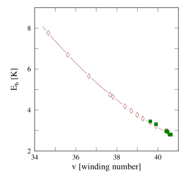
Figure 18: (Color online) The barrier energy $E_{\mathrm{b}}$ in kelvin vs $v$, the mean velocity in the aperture expressed in phase winding numbers and obtained from the nucleation rate data of Varoquaux and Avenel (2003): ($\scriptstyle{\blacksquare}$), low temperature data transformed using the numerical tables of Grabert et al. (1987); ($\lozenge$), high temperature data. From Varoquaux and Avenel (2003).

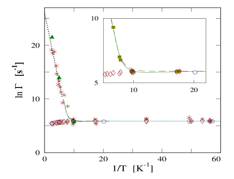
Figure 19: (Color online) Arrhenius plot $\ln\mathit{\Gamma}(v)$ vs $1/T$, $\mathit{\Gamma}$ being expressed in s^-1 and $T$ in kelvin, as measured at varying $T$ and $v_{\mathrm{c}}$ for two ultra-pure ⁴He samples ($\lozenge$) and ($\triangle$); ($\ast$) and ($\blacktriangle$) after correction for the change of the velocity with $T$. The plain and the dot-dot curves are calculated from the experimental barrier energy $E_{\mathrm{b}}$ represented in Fig.18. From Varoquaux and Avenel (2003). In the inset, $\ln\mathit{\Gamma}(v_{\mathrm{q}})$, ($\scriptstyle\blacksquare$), has been obtained with smoothed values of $v_{\mathrm{c}}$. The curves represent the calculated values of $\ln{\mathit{\Gamma}(v_{\mathrm{q}})}$ with $\alpha=0$ (dash-dash) or varying with $T$ (plain). The latter gives a better representation of the data and illustrates the influence of damping depicted by the dot-dot line in Fig.17.

The quantitative analysis can be carried out one step further using the variation of the barrier energy $E_{\mathrm{b}}$ in terms of $v$ to construct a Arrhenius plot – the logarithm of the escape rate $\mathit{\Gamma}$ in terms of the inverse temperature for a fixed potential well – from the experimental data and comparing directly the outcome to the results from theory. Arrhenius plots are drawn at constant $E_{\mathrm{b}}$ and varying temperature but the experimental results are obtained at velocities that vary with temperature, hence at varying $E_{\mathrm{b}}$. The correction can be computed from the experimentally determined $E_{\mathrm{b}}$ given in Fig.18. The final outcome for the nucleation rate data of Varoquaux and Avenel (2003) in ultra pure ⁴He is plotted in Fig.19.

As can be noted in Fig.19, the raw experimental, velocity-dependent rates exhibit little variation over the range of parameters: escape rates are only observed in a certain window determined by the measuring technique. At low temperatures, $T<T_{\mathrm{q}}$, the critical velocity is close to its zero temperature limit $v_{\mathrm{q}}$ and the corrections to $\mathit{\Gamma}$ are small. As $T$ increases above $T_{\mathrm{q}}$, $v_{\mathrm{c}}$ decreases and $\mathit{\Gamma}$ has to be determined by piece-wise integration of $\mathrm{d}\ln\mathit{\Gamma}/\mathrm{d}v$. The high temperature extrapolation for $\mathit{\Gamma}$ obtained in such a manner does display the usual $1/T$ dependence.

In the intermediate temperature range, the corrected $\mathit{\Gamma}$ shows, as can be seen in the inset of Fig.19, a small but real drop below its zero temperature limit as the temperature is raised. This drop reveals the influence of damping on the escape rate illustrated in Fig.17. A damping coefficient $\alpha$ that increases from 0 at $T=0$ to $\sim\,0.1$ around $T_{\mathrm{q}}$ and more slowly above accounts for the observed drop Varoquaux and Avenel (2003). This $T$-dependent dissipation also makes the crossover between the thermal and the quantum regimes even sharper than for $\alpha=0$, and closer to observations. The nucleation of vortices in ⁴He thus offers a rare observation of the effect of damping on MQT.

V.5 The vortex half-ring model

The case has been put so far for the nucleation of vortices, thermal or quantal. The nucleation barrier $E_{\mathrm{b}}$ is of the order of a few kelvins (see Fig.18) and the attempt frequency $\sim 2\times 10^{10}$ Hz, close to that of the highest Kelvin wave mode.

A simple model accounts for these features. This model – the nucleation of vortex half-rings at a prominent asperity on the walls – finds its roots in the work of Langer and Fisher (1967), Langer and Reppy (1970), Volovik (1972), and Muirhead et al. (1984). It was further developed and put on the firm experimental findings described above by Avenel et al. (1993).

The model premises are the following. Consider, as done by Langer and Reppy (1970), the homogeneous nucleation of a vortex ring in a homogeneous flow $v_{\mathrm{s}}$ extending over large distances. When the ring has grown to reach radius $R$ in a plane perpendicular to the flow, its energy in the laboratory frame, where the observer is at rest and sees the superfluid moving at velocity $v_{\mathrm{s}}$, is expressed by

$$E_{\mathrm{v}}=E_{\mathrm{R}}-P_{\mathrm{R}}v_{\mathrm{s}}\;.$$ (59)

The rest energy $E_{\mathrm{R}}$ and impulse $P_{\mathrm{R}}$ of the vortex ring are given by Eqs.(24) and (32). The minus sign in the right hand side of Eq.(59) arises because the vortex opposes the flow, that is, its impulse $P_{\mathrm{R}}$ points straight against $v_{\mathrm{s}}$: this configuration minimises $E_{\mathrm{v}}$.

Figure 20: Energy barrier $E_{\mathrm{v}}$ normalised by $\rho_{\mathrm{s}}\kappa_{4}^{2}a_{0}$ and expressed in kelvin vs the vortex radius $R/a_{0}$ for the vortex half-ring model. This figure illustrates various potential forms given by Eq.(59) at various superfluid flow velocities taken from the data in Fig.12 at, from top down, $T\rightarrow T_{\mbox{\footnotesize{l}}}$, 1 K, 0.5 K and at the quantum crossover $T_{\mathrm{q}}$. The lowest curve illustrates the situation in which the potential barrier vanishes and the trapped particle runs away, the so-called lability point. Adapted from Avenel et al. (1993).

The rest energy $E_{\mathrm{R}}$ increases with vortex size as $R\ln R$ and the impulse $P_{\mathrm{R}}$ as $R^{2}$: the impulse term becomes dominant at large radii and causes $E_{\mathrm{v}}$ to become negative. The variation of $E_{\mathrm{v}}$ in terms of $R$ has the shape of a confining well potential, which becomes shallower and shallower with increasing $v_{\mathrm{s}}$, as depicted in Fig.20. The barrier height can easily be computed numerically and plugged into the expression for $v_{\mathrm{c}}$, Eq.(48). An analytic approximation for $v_{\mathrm{c}}$ involving the neglect of logarithmic terms and valid for large vortices ($R\gg a_{0}$) has been given by Langer and Reppy (1970).

This critical process would yield a mist of vortices in the bulk of the superfluid. This sort of vorticity condensation does not take place for two reasons. First, the velocity of potential flows, which follows from the Laplace equation, reaches its maximum value at the boundaries, not in the bulk. Secondly, the nucleation of a vortex half-ring at the boundary itself involves, for the same radius hence the same self-induced velocity, a half of the energy given by Eq.(59); for that reason alone, half-ring nucleation at walls is always much more probable at the same velocity $v_{\mathrm{s}}$ than full ring nucleation in the bulk.

Halving the full-ring energy for the half-ring holds for classical hydrodynamics, the other half being taken care of by the image in the plane boundary. For a superfluid vortex, the actual energy of a half-ring is smaller than in the classical ideal fluid because the superfluid density is depleted at the solid wall and the core radius increases.

The half-ring model for the nucleation of vortices has been proposed for ion critical velocity by Muirhead et al. (1984) and for aperture flows by Burkhart et al. (1994). A variant, based on a different accounting of the vortex core energy, has been studied by Zimmermann, Jr. et al. (1998). Other mechanisms have been discussed Josserand and Pomeau (1995); Josserand et al. (1995); Andreev and Melnikovsky (2004) for which it is unclear that the end product of the nucleation process is actually a vortex.

The barrier height for the vortex half-ring nucleation can easily be computed and plugged into the expressions for $v_{\mathrm{c}}$ and $\Delta v_{\mathrm{c}}$, Eqs.(48) and (49). Critical velocities $v_{\mathrm{c}}$ and statistical widths $\Delta v_{\mathrm{c}}$ computed in such a manner are shown as a function of temperature by the solid lines in Figs.12 and 13 for several values of the vortex core parameter $a_{0}$. A value of 4.5 Å gives near-quantitative agreement with the experimental observations over the entire temperature range. This value exceeds that in the bulk ($a_{0}\simeq 2.5$ Å). This is thought to reflect the proximity of the wall as discussed by Varoquaux et al. (2001). With this value, the nucleating half-ring has a radius of approximately 15 Å at the top of the barrier and a self-velocity of $v_{\mathrm{R}}=13.5$ m/sec from Eq.(33); this value compares well with the values shown by open circles in Fig.11.

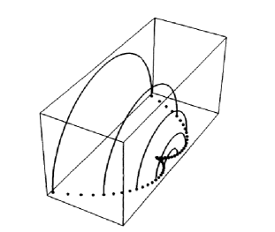
Figure 21: Schematic views in 2D (top) and 3D (bottom) of the vortex half-ring trajectory over a point-like pinhole punched in an infinite horizontal plane. The dashed lines on the 2D plot are the potential flow streamlines that emerge from the pinhole. The 3D view shows the vortex half-ring being first pushed by the potential flow to the right and then flying back over the pinhole to finally drift away to the upper left. Adapted from (Varoquaux, 2006).

Once nucleated, the vortex half-ring floats away, carried out by the superfluid stream at the local superfluid velocity and by its own velocity, $v_{\mathrm{R}}=\partial E_{\mathrm{R}}/\partial P_{\mathrm{R}}$. It can be noted that, at the top of the barrier, $\partial E_{\mathrm{v}}/\partial R=0$: the vortex self-velocity $v_{\mathrm{R}}$ exactly balances the applied $v_{\mathrm{s}}$; the nucleating vortex is at a near standstill.

If the flow were uniform, with parallel streamlines, nothing much would happen. Downstream from the aperture however, the flow is divergent, as pictured in Fig.21. The vortex half-ring tends to follow the local streamlines and grow under the combined action of the potential flow and its own self-velocity: it then gains energy at the expense of the potential flow as explained in §II.3. In such a way, it expands from nanometric to micrometric sizes and above, and wanders away. Interaction with the normal fluid, encounters with other vortices and friction on the solid boundaries cause a loss of vortex energy that eventually leads to its disappearance. The vortex in its motion away from the micro-aperture takes a given finite lump of energy to remote places of the cell and never returns.

This scenario for a phase slip produces a change of the phase difference between the two sides of the micro-aperture of exactly $2\pi$ because the vortex ends up crossing all the streamlines, as pictured in Fig.21. This crossing causes the velocity circulation to change by exactly one quantum $\kappa_{4}$ on all the superfluid paths extending from one side of the aperture to the other. Such a dissipative event gives the signature of single phase slips that are seen in Fig.10. Extensive numerical simulations by Schwarz (1993b, a) and Flaten et al. (2006a) fully confirm the above scenario for phase slips.

The effect of ³He impurities on the phase slip critical velocity at low temperature is striking, as seen in the inset of Fig.12. It is due to the condensation of these impurities on the vortex cores, which changes their line energy and the potential barrier for nucleation. This impurity dependence, studied in detail by Varoquaux et al. (1993), was used as a local probe of the superfluid velocity at which vortices nucleate. This velocity was found to be 22 m/s, an important piece of information in reasonable agreement with the value derived from the vortex half-ring model.

In all, the model parameters hang fairly well together, showing that specific finer details are probably not very relevant and that the model simplifications are reasonably well founded. It nonetheless remains that the nature and geometry of a typical nucleation site are wholly unspecified and that the enhancement factor between the mean aperture velocity and the velocity at the nucleation site is not under control, as shown in particular by Shifflett and Hess (1995).

VI Vortex pinning, mills and flow collapse

Single phase slips are observed in experimental situations that may be loosely characterised as “clean”, broadly speaking for uncontaminated apertures of relatively small sizes (a few micrometres at the most), with low background of mechanical and acoustical interferences …, and with probing techniques that do not manhandle the superfluid, namely, with low frequency hydromechanical resonators.

When these conditions are not met, flow dissipation occurs in a more erratic manner in large bursts – multiple phase slips or “collapses” of the superflow. Such collapses of the superflow through an orifice were first observed by Sabo and Zimmermann, Jr. and by Hess (1977).

Multiple phase slips and collapses constitute an apparent disruption of the vortex nucleation mechanism described in the previous Section. Their properties have been studied in detail by Avenel et al. (1995) and are briefly mentioned below, together with possible mechanisms for their formation. It is likely that these events provide a bridge between the “clean” single phase slip case and the usual situation of the Feynman-type critical velocities that are temperature-independent below 1 K and dependent on the channel size. Preexisting vorticity is widely suspected to come into play in these “extrinsic” critical velocities.

VI.1 Pinned vorticity

Awschalom and Schwarz (1984) have directly shown the existence of remanent vorticity in ⁴He, which had long been assumed, and have given an estimate of its background level. These authors studied the propagation of ions in the presence of vortex lines. Ions get trapped in the vortex cores and completely change course, revealing the presence of these vortex lines. These vortices, presumably nucleated at the l transition when the critical velocity is low and critical fluctuations large, remain stuck in various places of the superfluid sample container. This trapped vorticity, according to Adams et al. (1985), either is quite loosely bound to the substrate and disappears rapidly, or is strongly pinned and dislodged only by strong perturbations.

To achieve a stable configuration, a pinned vortex has to take on a shape such that its local radius of curvature results in a self-velocity that exactly opposes at each of its points the local value of the superflow. This dynamic equilibrium is what is meant here by pinning. Vortex pinning exists in bulk ⁴He as discussed here, in films, in ³He, in neutron stars …

To account for laboratory observations and with the outcome of extensive numerical simulations of vortex dynamics, Schwarz has proposed the following formula for the velocity at which such strongly pinned vortices unpin Schwarz (1981, 1985),

$$v_{\mathrm{u}}\lesssim\frac{\kappa_{4}}{2\pi D}\,\ln\left(\frac{b}{a_{0}}\right)\;,$$ (60)

$D$ being the size of the pinned vortex and $b$ being a characteristic size of the pinning asperity. Equation (60) bears a strong resemblance with that for the Feynman critical velocity, Eq.(45).

As a rule of thumb, the pinning energy of the vortex line on such an asperity with radius $b$ is approximately equal to $b$ times the line tension of the vortex given by Eq.(26). Long vortices unpin at very low velocities unless they are perched on a tall pedestal, but very small vortices pinned on microscopic defects can survive a wide range of superflow velocities; according to Eq.(60), a straight vortex filament pinned at both ends on 20 Å asperities 200 nm apart resists transverse flows of velocities up to 20 cm/s.

Such pinned vorticity has long been thought to play a role in critical velocities. The long standing suggestion by Glaberson and Donnelly (1966) of vortex mills had its time of fame (Amar et al., 1992). In these authors’s  views, imposing a flow on a vortex pinned between the opposite lips of an aperture would induce deformations such that the vortex would twist on itself, self-reconnect, and mill out fresh vortex loops. Upon scrutiny however, vortex mills are not so easy to set up.

The first thing to realise is that such a mill must involve a pinned vortex of sub-micrometric size so that it is not washed away by any flow velocity above a few cm/s. Pinned vorticity in large channels cannot withstand the Feynman-type critical velocities shown in Fig.11.

Less obviously, vortices are not prone to twist on themselves and foster loops. As shown by numerical simulations of 3D flows involving few vortices only, vortex loops and filaments are found to be stable against large deformations: it takes the complex flow fields associated with fully developed vortex tangles to produce small rings (Svistunov, 1995; Tsubota et al., 2000). And it takes some quite special vortex pinning geometry to set up a mill that actually works.

Schwarz (1990) has demonstrated the existence of such a mill by numerical simulations. Imagine a vortex filament pinned at one end in a region close to the aperture mouth or the channel entrance where it bends sharply to withstand the local superflow. This end of the vortex is at a near-stagnation point. Its other end is being carried away by the flow along the streamlines; it moves freely with its end sliding perpendicular to the wall. The filament develops a helical instability as depicted in Fig.22, a sort of driven Kelvin wave, and reconnects sporadically to the wall when the amplitude of the helix grows large enough. The freed bit immediately stands against the flow and forms a vortex half-ring: such a helical vortex mill, which has to be of sub-micrometric size to withstand the near-by flow, does churn out fresh vortices.

The occurrence of multiple slips such as those shown in Fig.23, is probably caused by such a form of vortex mill on a microscopic size. Before coming to this topic, a description of multiple slips in greater details must be provided.

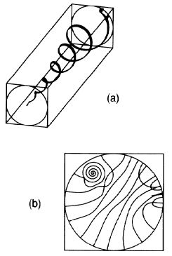
Figure 22: Operation of a helical vortex mill: (a) Spiral-helix configuration of a streamwise vortex filament pinned at the centre of the bottom left section of the channel. The helical vortex self-velocity opposes the superflow while the vortex filament grows in size and spirals on itself. (b) End-on view of subsequent reconnections. The vortex is pinned near the upper left of the channel cut view. The outwardly growing spiral sporadically reconnects to the wall and releases a new line segment, which then moves to the lower right. These numerical simulations are carried out in the presence of a sizeable mutual friction with the normal component in order to stabilise the numerical algorithms, which is why the generated half-rings rapidly decrease in size. From Schwarz (1990).

VI.2 The two types of large slips

Examples of multiple slips are shown on the peak amplitude charts in Fig.23 and in Fig.24 for two different runs in the same experimental cell. They display rather different patterns. In Fig.23, multiples slips are fairly frequent and their winding number multiplicity remains moderate. As the probability for a one-slip event per half-cycle is not large, that for a double slip is small, and it becomes negligible for higher multiples. A separate mechanism for their formation must be found. The event shown in Fig.24 is quite spectacular as it leads to a near-extinction of the resonance.

In Figs. 23 and 24 aperture velocities are expressed by the number of turns $\delta\varphi/2\pi$ by which the quantum-mechanical phase winds across the aperture. Phase winding numbers are related to mean flow velocities in cm/s by multiplication by $\ell_{\mathrm{h}}/\kappa_{4}$, the “hydraulic” length $\ell_{\mathrm{h}}$ characterising the extension of the aperture along the flow. For a phase slip by 2$\pi$, the phase winding number changes by one unit and the trapped circulation in the resonator loop by one quantum.The hydraulic length is defined by lumping the (classical) kinetic energy of the fluid moving with velocity $\mathbf{v}$ inside the aperture of cross-section $s_{\mathrm{h}}$ and in its vicinity according to:

$$\ell_{\mathrm{h}}=s_{\mathrm{h}}\,\int_{V}\mathbf{v}(\mathbf{r})^{2}\mathrm{d}^{3}\mathbf{r}\,\big{/}\,\big{(}\int_{S}\mathbf{v}(\mathbf{r})\cdot\mathrm{d}^{2}\mathbf{r}\big{)}^{2}\;.$$ (61)

The actual flow velocity averaged over the cross-section of the micro-aperture is proportional to $\delta\varphi$, the multiplying factor being $\hbar/m_{4}\ell_{\mathrm{h}}$. The hydraulic length $\ell_{\mathrm{h}}$ of the micro-aperture is of the order of 1 mm in the experiments shown in Fig.10.

Some degree of understanding of the formation of multiple slips can be gained by plotting the mean value of the phase slip multiplicity, expressed in number of quanta, against the flow velocity at which the slips take place Varoquaux et al. (1995). This flow velocity is close to the critical velocity for single phase slips, i.e. the vortex nucleation velocity; it varies with temperature, pressure, and resonator drive level. A plot summarising these variations is shown in Fig. 25 for $<\!n_{{}_{+}}\!\!>$, i.e., in the flow direction conventionally chosen as the $(+)$ direction. Slips in the opposite $(-)$ direction behave qualitatively in the same manner but the phenomenon displays a clear quantitative asymmetry.

As can be seen in Fig. 25, the mean slip multiplicity decreases, as does the nucleation velocity, on either side of the quantum plateau – a ³He impurity effect on the low–$T$ side – a thermal effect on the high–$T$ side. At 16 bars, $<\!n_{{}_{+}}\!\!>$ increases from $\approx 1$ at 12 mK where the velocity is 43.2 in winding number to $15\sim 20$ on the plateau of $v$ with a winding number of 48; $<\!n_{{}_{+}}\!\!>$ drops back to 1 at 225 mK and the velocity to $\sim 46.2$. The same trend is observed at 24 bars, with a lower velocity on the plateau of 46.4 and a higher mean multiplicity of $\sim$ 23. Rather oddly, the slip multiplicity $<\!n_{{}_{+}}\!\!>$ increases with pressure while the mean velocity at which these multiples occurs decreases. One would have expected – naively it seems – that more slips would be ushered into faster streams. The opposite may show that the phenomenon under study is not purely ruled by hydrodynamics in the fluid bulk.

Another important feature of the data shown in Fig. 25 concerns the dependence of the velocity threshold for the appearance of multiple slips on hydrostatic pressure. The $P$-dependence of the upturn of $<\!n_{{}_{+}}\!\!>$ in terms of $v$ exactly tracks that of $v_{\mathrm{c}}$, the critical velocity for single phase slip nucleation: multiple slips occur when single slips occur. Would multiple slips appear because of an alteration, or as a consequence, of single slip nucleation?

The very large drops in the resonance amplitude of the resonator such as the event shown in Fig.24 and in the inset sometimes result in a complete collapse of the resonance. Under the conditions of this particular exper-

Figure 23: Absolute peak amplitude $A_{\mathrm{p}}$ normalised to the amplitude jump of a single slip $\Delta A_{1}$ during successive half-cycles of the resonance plotted as a function of half-cycle index (time runs from left to right) at 100.7 mK (top) and 201.5 mK (bottom) in nominal purity helium at SVP. The expanded traces at the very top and bottom of the graph show the slip sizes in signed winding numbers (according to flow direction, in and out of the resonator chamber). The numerous multiple slips seen on these charts occur at or close to the critical velocity for single slips. From (Varoquaux and Avenel, 2003).

iment (Avenel et al., 1995), these events were rare (one in $10^{4}\mbox{ to }10^{5}$ slips). A striking feature is that they may occur at velocities much below the vortex nucleation threshold, down to less than a third of $v_{c}$, the critical velocity for phase slips. These intriguing “singular” collapses, first studied by Hess (1977), differ from the multiple slips of Fig.25. The underlying mechanisms responsible for each are bound to be different, as discussed below Varoquaux et al. (2001).

The pattern of formation of multiple slips and collapses changes on cycling the cell from room temperature and back but remains stable during each given cool-down. It depends on the degree of contamination of the cell, degree which cannot easily be controlled experimentally. The detailed microscopic configuration of the aperture wall where nucleation takes place has a strong influence on multiple slip formation.

Figure 24: Absolute peak amplitudes at successive half-cycles of the resonator motion, normalised as in Fig.23, vs half-cycle index in a ⁴He sample containing 100 ppb of ³He impurity, at 24.0 bars and 12.5 mK. The resonance half-period is 31.8 msec. The top trace shows a succession of amplitude drops which correspond, for its main part, to phase slips by $2\pi$ of opposite sign, with occasional larger slips – the multiple slips of Fig.23. The large feature around the 1000^th half-cycle is a “singular” collapse, as defined in this Section. The insert shows the details of this collapse, ($\bullet$) being for positive peaks, ($\circ$) for negative peaks. It is preceded by a slip by -2 ($\times 2\pi$) and followed by a slow recovery of the peak amplitude caused by the applied drive, punctuated by single and double slips. The time-resolved evolution of this collapse has actually been tracked. See Avenel et al. (1995).

Figure 25: Mean size of (positive) multiple slips vs velocity in phase winding number in nominal purity ⁴He (100 ppb ³He): ($\triangle$) pressure sweep from 0.4 to 24 bars at 81.5 mK (for all even values of the pressure $P$, and 0.4, 1, 3, 5, and 7 bars) – ($\diamond$) temperature sweep at 16 bars – ($\circ$) temperature sweep at 24 bars - ($\ast$) drive level sweep at 24 bars, 81.5 mK – ($\scriptscriptstyle\blacksquare$) temperature sweep at 0 bar. Lines connect successive data points in the temperature and pressure sweeps. For the temperature sweeps, from 14 to 200 mK approximately, $v$ first increases when the ³He impurities evaporate from the vortex core, reaches the quantum plateau and then decreases, following the same pattern as shown in the insert of Fig.12 for $v_{\mathrm{c}}$. Adapted from Varoquaux et al. (2001).

VI.3 Extrinsic critical velocities

To try and clarify these matters, a series of experiments was conducted by Hakonen et al. (1998)Varoquaux et al. (1998), in which the experimental cell was deliberately heavily contaminated by atomic clusters of air and of H₂ in order to favour the pinning of vortices. Numerous multiple slips and collapses of the “singular” type occurred. The peak amplitude charts of the resonator became very difficult to interpret except in few instances. In one of these, two apparent critical velocities for single phase slips were observed. The higher critical velocity corresponded to the one observed in the absence of contamination. The lower critical velocity was thought to reveal the influence of a vortex pinned in the immediate vicinity of the prevailing nucleation site.

Following this interpretation, the pinned vortex induces a local velocity which adds to that of the applied flow and causes an apparent decrease in the critical velocity for phase slips. Because of this change, the presence of the pinned vortex can be monitored. The lifetime in the pinned state and the unpinning velocity can be measured, yielding precious information on the pinning process, reported in detail by Hakonen et al. (1998).. This observation also brings evidence that pinned vorticity can alter the vortex nucleation process responsible for phase slips.

With such pinned vortices hanging around, multiple slips could formed according to the following scheme (Varoquaux et al., 2001). First, a vortex half-ring is nucleated at a prominent nucleation site. It pins shortly after nucleation when its velocity relative to the boundary is still small and the capture by a pinning site easy. A micro-mill is thus formed, which remains active as long as the flow is sufficient to maintain the helical instability. As it is set up to withstand one flow direction, it is destroyed when the flow velocity reverses itself in the resonance motion. It eventually re-establishes itself during a subsequent resonance cycle, causing a new multiple slip. This process depends on the precise details of the pinning site configuration and of the primordial vortex trajectory, factors which allow for the variableness of multiple slips on contamination and pressure.

In the same experiments by Hakonen et al. (1998), a large number of unpinning events were also observed to take place at an “anomalously low” unpinning velocity. A parallel can be made (Varoquaux et al., 1998) with the singular collapses that also occur at “subcritical” velocities and that were also quite frequent in the same experiments, suggesting that the two effects might have a common cause. Noting furthermore that pinning and unpinning processes were also quite frequent, releasing a fair amount of vagrant vorticity, it appears quite plausible that both singular collapses and low velocity unpinning events are caused by vagrant vortices hopping from pinning sites to pinning sites, eventually hovering over a pinned vortex or a vortex nucleation site. The transient boost to the local velocity may push the pinned vortex off its perch, or may cause a burst of vortices to be shed.

These observations, albeit incidental, have important consequences for the critical velocity problem: existing vortices, either pinned or free-moving, can contribute to the nucleation of new vortices at the walls of the experimental cell at apparent velocities much lower than the critical velocity for phase slips. A mechanism is thus provided by which superflow dissipation sets in at large scale for mean velocities much smaller than the velocity for vortex nucleation on the microscopic scale, possibly bridging the gap between phase slip and Feynman-type critical velocities.

To conclude this Section, the critical velocities in superfluids that are true and proven include the Landau critical velocity for roton creation in ion propagation McClintock and Bowley (1995), the formation of vortices by a hydrodynamical instability in BEC gases Madison et al. (2001) and in ³He Eltsov et al. (2005), the nucleation of vortices by thermal activation and quantum tunnelling in ⁴He, both for ion propagation and in aperture flow.

There is also rather compelling experimental evidence for the interplay on a microscopic scale between vortex nucleation and pinned vorticity; this evidence points toward the existence of helical vortex micro-mills that can generate bursts of vortices, even, in some cases, at fairly low flow velocities. Finally, vagrant vortices interacting with these mills, or with the vortex nucleation sites are found to generate enough vorticity to completely kill the superflow and explain singular collapses.

How these different events occur is illustrated in detail by the numerical simulations of the onset and decay of vortex tangles in large channels Schwarz (1983); Schwarz and Rozen (1991), of the influence of surface roughness on the critical velocity for a self-sustaining vortex tangle Schwarz (1992), and of the evolution of phase-slip cascades from a single remnant vortex as a function of channel size Schwarz (1993b). These processes depend on the cell geometry but not on temperature.

A fair degree of understanding of the possible mechanisms behind the Feynman critical velocity has thus been achieved by the study of phase slippage signatures of these various large slips.

VII Josephson-type effects in superfluids

Anderson’s conjectures, seen in the previous Sections to be fully confirmed in the hydrodynamic (macroscopic) limit of quantised vortex dynamics, have also been carried over to the microscopic limit of quantum tunnelling, as described below.

The reasoning goes that Eqs.(12) and (13) are fundamental  enough to carry the day both at large and short distances, namely when the coherence length is either small or large with respect to characteristic dimensions of the hydrodynamic weak link. The former case has been covered in the previous Sections. In the latter case – weak quantum coupling between two superfluid baths – the contention is that effects analogous to the famed Josephson effects between two weakly-coupled bits of superconducting material must also exist between two loosely-connected pools of superfluid provided that superfluid coherence is not entirely lost through the connection. These Josephson-type effects in superfluids are dealt with below.

VII.1 A simple model

The Hamilton equations (12) and (13) express in a quite general way the time evolution of $\varphi$ and $N$, as discussed in Sec.I.2. These equations hold in fact for the operators $\hat{N}$ and $\hat{\varphi}$ but their coarse-grained averages can be treated as c-numbers to a very good approximation because their relative quantum uncertainties are very small. Averaging over a volume of superfluid small compared to the size of the sample but still containing a large number of atoms leads to Eq.(14):

$$\hbar\frac{\partial\varphi}{\partial t}=-(\mu+\kern 1.00006pt^{1}\kern-3.00003pt/\kern-1.00006pt_{2}m_{4}v_{\mathrm{s}}^{2})\;.$$

Equation (14) describes the Josephson ac effect.

Figure 26: Schematic representation of a two–dimensional weak link: (top) cut view of the elongated slit in the partitioning wall; (bottom) amplitude of the macroscopic wavefunction $\Phi$ in the region in which it is depleted by the energy barrier of height $U$ and extent $l_{\mathrm{b}}$ due to the constricting walls.

When applied to the gradient of the phase, it can be cast, using Eq.(6), into the Euler equation (15):

$$\frac{\partial\mathbf{v}}{\partial t}+\nabla(v_{\mathrm{a}}P+\frac{1}{2}m_{\mathrm{a}}v^{2})=0\;,$$

$m_{\mathrm{a}}$ being the atomic mass of the effective boson.

Equations (14) and (15) look plainly classical enough. Quantum mechanics hides in the possible multiple determinations of the overall phase $\varphi(t,\mathbf{r})$ of the order parameter, yielding a quantised circulation of the fluid velocity, and, in a subtler manner, when $\hat{N}$ cannot be coarse-grained averaged because the amplitude of the order parameter vanishes or varies too rapidly over short distances. A (quantum) mechanism is then provided for $\varphi$ to vary discontinuously from one determination to another, violating the Kelvin-Helmholtz theorem.

The second Heisenberg equation of motion, that for $\dot{N}$, expresses particle number conservation:

$$\hbar\,\frac{\partial N}{\partial t}=\frac{\partial E}{\partial\varphi}\;.$$ (62)

As stressed by Anderson (1966a), the range of validity of Eqs.(14) and (62) is quite wide. They will still hold when hydrodynamics breaks down as for tunnelling supercurrents. In this kind of situations, the internal energy $E$ depends in a non-trivial way on $\varphi$, as may be expected from Eq.(62).

When applied between two regions of the superfluid, Eqs.(14) and (62) describe the supercurrent flowing from one region to the other. This situation becomes especially interesting when the two regions, the two superfluid baths, are sufficiently well separated so that they only weakly coupled: a well-defined phase difference between them, $\mbox{{d}}\varphi$, can then be sustained.

Such a situation can be modelled by a potential barrier, as in Fig.26. The thin partition separating the two baths presents a thin elongated slit through which a trickle flow only of superfluid can leak. If the two smaller dimensions of the slit are comparable to the superfluid coherence length — the distance over which its wavefunction can heal — the amplitude of the wavefunction is reduced in the narrow passage, as pictured in the bottom panel of Fig.26. In superconductivity, such weak links, or micro-bridges, are known to lead to the same kind of effects as tunnel junctions Likharev (1979); Golubov et al. (2004).

For superflows through such a micro-aperture, the problem can be restricted to one dimension along $z$ and, to simplify further, the barrier (the weak link) can be taken as a square potential wall of height $U$ over length $l_{\mathrm{b}}$.

In the bulk of the fluid, the wave function corresponding to a state with energy $E$ is taken as a plane wave with identical amplitude $|\mathit{\Phi}|=(\rho_{\mathrm{s}}/m_{\mathrm{a}})^{1/2}$ on both sides of the barrier ($m_{\mathrm{a}}=2m_{3}$ for superfluid ³He), but with phases that differ by $\mbox{{d}}\varphi$: these are the boundary conditions at the weak link walls at $z=0$ and $z=l_{\mathrm{b}}$.

Inside the barrier $|\mathit{\Phi}(z)|$ is assumed to be severely depressed: the interactions within the fluid can be neglected. With this approximation of weak coupling, the tenuous fluid inside the weak link behaves as a simple non-interaction gas and the equation of motion reduces to a one-particle Schrödinger equation:

$$\mathrm{i}\hbar\frac{\partial\mathit{\Phi}}{\partial t}=-\frac{\hbar^{2}}{2m_{\mathrm{a}}}\nabla^{2}\mathit{\Phi}+U\mathit{\Phi}\;,\hskip 5.69054ptU>E\;,$$

and also has a plane wave solution $\exp\{-\mathrm{i}(Et/\hbar-kz)\}$. The momentum takes two values corresponding to the two possible directions of (damped) propagation:

$$k_{\textstyle{\pm}}=\pm(\mathrm{i}/\hbar)\sqrt{2m_{\mathrm{a}}(U-E)}\;.$$

Let $b_{\mathrm{b}}=\hbar/\sqrt{2m_{\mathrm{a}}(U-E)}$ : the barrier height is characterised by a penetration length. The wave function inside the barrier is found by standard methods:

$$\mathit{\Phi}(z)=\frac{|\mathit{\Phi}|}{{\sinh}(l_{\mathrm{b}}/b_{\mathrm{b}})}\left\{{\sinh}\left(\frac{z}{b_{\mathrm{b}}}\right)\,{\mbox{e}}^{\textstyle{\mathrm{i}\mbox{{d}}\varphi}}-{\sinh}\left(\frac{z-l_{\mathrm{b}}}{b_{\mathrm{b}}}\right)\right\}\;.$$

The modulus of $\mathit{\Phi}$ midway in the barrier is expressed by

$$\mathit{\Phi}^{*}(l_{\mathrm{b}}/2)\,\mathit{\Phi}(l_{\mathrm{b}}/2)=\frac{\rho_{\mathrm{s}}/m_{\mathrm{a}}}{2\cosh^{2}(l_{\mathrm{b}}/2b_{\mathrm{b}})}[1+\cos\mbox{{d}}\varphi]\;,$$ (63)

and is a $2\pi$-periodic function that vanishes for $\mbox{{d}}\varphi=\pi\,\pm 2n\pi$. The weak coupling condition is satisfied in superfluid helium for $l_{\mathrm{b}}\gtrsim b_{\mathrm{b}}$.

Knowing the wavefunction, the current density, Eq.(5), can be straightforwardly computed. The total current through a micro-aperture of effective cross-section $s_{\mathrm{b}}$ is found to be:

$$J = \frac{\hbar s_{\mathrm{b}}}{2\mathrm{i}b_{\mathrm{b}}}\frac{\rho_{\mathrm{s}}/m_{\mathrm{a}}}{{\sinh}^{2}\left(l_{\mathrm{b}}/b_{\mathrm{b}}\right)}\left\{\left[{\sinh}\left(\frac{z}{b_{\mathrm{b}}}\right)\,{\mbox{e}}^{\textstyle{-\mathrm{i}\mbox{{d}}\varphi}}-{\sinh}\left(\frac{z-l_{\mathrm{b}}}{b_{\mathrm{b}}}\right)\right]\times\right.$$ (64)

$$\hskip-14.22636pt\left.\left[{\cosh}\left(\frac{z}{b_{\mathrm{b}}}\right){\mbox{e}}^{\textstyle{\mathrm{i}\mbox{{d}}\varphi}}-{\cosh}\left(\frac{z-l_{\mathrm{b}}}{b_{\mathrm{b}}}\right)\right]-{\mbox{complex conjugate}}\right\}$$

$$= J_{\mathrm{c}}\,\sin\left(\mbox{{d}}\varphi\right)\,,\;\;{\mbox{with}}\;J_{\mathrm{c}}=\frac{\hbar}{m_{\mathrm{a}}}\,\frac{s_{\mathrm{b}}}{b_{\mathrm{b}}}\,\frac{\rho_{\mathrm{s}}}{{\sinh(l_{\mathrm{b}}/b_{\mathrm{b}})}}\;.$$

Equation (64) describes the Josephson dc effect. Although this equation has been obtained here in a drastically simplified manner, it is nearly identical to the result of more involved theories, each with its own set of approximations – the Ginzburg-Landau model Monien and Tewordt (1986), an ideal tunnel junction Rainer and Lee (1987), or a strictly point-like orifice Kurkijärvi (1988).

The supercurrent $J$ is periodic by $2\pi$ in $\mbox{{d}}\varphi$ as it must be since changing the phase by $2\pi$ on one side of the barrier must leave the overall physical situation unchanged. It vanishes for $\mbox{{d}}\varphi=\pm\pi$ not because the velocity, proportional to $\mbox{{d}}\varphi$, goes to zero but because the superfluid density, which is proportional to $|\mathrm{\Phi}|^{2}\sin(\mbox{{d}}\varphi)/\mbox{{d}}\varphi$ inside the barrier, does; the modulus of the wave function at midpoint in the barrier, Eq.(63), vanishes: superfluidity is actually destroyed at that point, which is why the supercurrent goes to zero and the phase can slip by $2\pi$ (or lumps of $2\pi$).

If the coupling is not weak, a more elaborate calculation is necessary: the sine function is replaced by a general $2\pi$–periodic function $f_{2\pi}(\mbox{{d}}\varphi)$, the current-phase relation, or CPR, for a “non-ideal” weak link. Often, this relation is not even single-valued and, when the phase is varied, the current may jump discontinuously from one determination to another: the weak link is then said to be hysteretic. This behaviour is due to the nucleation of topological defects such as vortices as seen in the previous Section. It is accompanied by dissipation while the ideal Josephson case (when $f_{2\pi}(\mbox{{d}}\varphi)$ is a sine function) is dissipation-less Likharev (1979); Thuneberg (2005); Viljas (2005).

In the transition between the “ideal”, non-hysteretic, purely sinusoidal CPR’s and the mostly linear CPR seen, for example, in Fig.10, a slanted sine function is often observed. Part of this distortion arises from purely classical fluid flow in the vicinity of the micro-aperture. The full phase difference across the weak link, $\varphi_{\mathrm{w}}$, includes, besides the phase difference across the barrier $\varphi_{\mathrm{b}}$, the rather trivial velocity potential drop in the vicinity of the weak link where the superfluid velocity $v_{\mathrm{s}}$, and the corresponding phase gradient, behave in accord with classical ideal fluid dynamics.

In order to account in a simple manner for this classical contribution, it is convenient to introduce the equivalent "hydraulic" length and cross-sectional area of these regions, $\ell_{\mathrm{h}}$ and $s_{\mathrm{h}}$, in such a way that the flow is described in a ‘rod-like” manner.. The superfluid velocity is then expressed simply by $v_{\mathrm{s}}=(\hbar/m_{\mathrm{a}})\mbox{\small{d}\hskip 0.19376pt}\varphi_{\mathrm{h}}/\ell_{\mathrm{h}}$ and the current by $J=\rho_{\mathrm{s}}s_{\mathrm{h}}v_{\mathrm{s}}$.

The total phase difference $\mbox{\small{d}\hskip 0.19376pt}\varphi$ is the sum of the phase drop through this "hydraulic" region and through the barrier acting as the weak link, assumed ideal, i.e., such that:

$$\mbox{\small{d}\hskip 0.19376pt}\varphi=\mbox{\small{d}\hskip 0.19376pt}\varphi_{\mathrm{h}}+\mbox{\small{d}\hskip 0.19376pt}\varphi_{\mathrm{b}}=\frac{m_{\mathrm{a}}\ell_{\mathrm{h}}}{\rho_{\mathrm{s}}\hbar s_{\mathrm{h}}}\,J\;.$$ (65)

The same mass current also flows through the depletion region and varies, following Eq.(64), as a sine function of the phase difference $\mbox{\small{d}\hskip 0.19376pt}\varphi_{\mathrm{b}}$ as long as the coupling is weak.

Combining Eqs.(64) and (65), and renaming the hydraulic part $\mbox{\small{d}\hskip 0.19376pt}\varphi_{\mathrm{h}}$ of the phase difference $\zeta$ to stress its ancillary role yields the relation between the current and the phase of a (slightly more) realistic micro-aperture:

$$\varphi=\zeta+\alpha\sin\zeta\;,\;\;\;\;\;\ J=J_{\mathrm{c}}\sin\zeta\;,$$ (66)

with $\alpha=(m_{\mathrm{a}}\ell_{\mathrm{h}}/\rho_{\mathrm{s}}s_{\mathrm{h}}\hbar)\,J_{\mathrm{c}}$ and $J_{\mathrm{c}}$ expressed from Eq.(64). The non-ideality parameter $\alpha$ and the critical current through the junction $J_{\mathrm{c}}$ are given a meaning in terms the geometrical details of the micro-aperture. They can be derived from experiments and compared with the expected values.

Since the healing length is of atomic dimensions for ⁴He, a near-ideal Josephson effect cannot be expected to be found in the micro-apertures that can be manufactured at present, except very close to the l transition when this length diverges. Experiments close to $T_{\mbox{\footnotesize{l}}}$ have been conducted successfully by Sukhatme et al. (2001) and Hoskinson et al. (2006a) and are described in §VII.6. The experiments that have first shown the existence of the Josephson dc-effect in superfluids have been carried out in ³He (Avenel and Varoquaux, 1988).

VII.2 Current and phase in superfluid ³He

The helium-3 nucleus is made up of two protons and one neutron: ³He is a fermion. As for the abundant and heavier isotope, ⁴He, its zero-point energy in the condensed phase is large and it remains in the liquid phase down to absolute zero at pressures below about 35 bars. It thus forms a Fermi liquid with a Fermi sphere over which Landau quasiparticles float. Because the interatomic potential is attractive at large distance, these quasi-particles can form Cooper pairs and ³He was long suspected to become a BCS superfluid below some hard-to-predict temperature. The discovery by Osheroff, Richardson and Lee of the transition to not one but two superfluid phases (Osheroff et al., 1972) fixed the transition temperature to 2.49 mK on the melting curve, at a pressure of 34.34 bars and opened an exciting new chapter of low temperature physics.

As the experimental properties of these new superfluid phases were quickly unravelled (Wheatley, 1975a, b; Lee and Richardson, 1978), they were identified from their nuclear susceptibility properties observed by NMR as resulting from the formation of Cooper pairs in a spin-triplet state (Leggett, 1975). A new breed of superfluid was just born. The overall antisymmetry of the wavefunction under the exchange of two fermions then requires an odd angular momentum state $l=1,\,3\,\ldots$. The available experimental data, mainly the phase diagram, the specific heat, and the nuclear susceptibility, led to the identification of the A and B phases as p-wave Cooper-pair superfluids with total spin $S=1$ and total angular momentum $L=1$.

The formalism describing the properties of these anisotropic superfluid phases was quickly developed. It extended the Bardeen-Cooper-Schrieffer theory of s-wave superconductivity to the neutral triplet-spin-state superfluid. The most general pair wavefunction with three possible substates for the spin and the orbital parts is an arbitrary superposition of these 3x3 substates, involving nine complex parameters. Assuming weak coupling between the pairs – a surprisingly good assumption at low pressure – this extension of the BCS theory (Leggett, 1975) leads to a 3x3 order parameter for B-phase of the form

$$A_{\mu i}=\Delta(\hat{\boldsymbol{\mathrm{k}}})\mathrm{e}^{\textstyle{\mathrm{i}\varphi}}\,R_{\mu i}(\hat{\boldsymbol{\mathrm{n}}},\theta)\;.$$ (67)

The gap parameter $\Delta(\hat{\boldsymbol{\mathrm{k}}})$ and the phase factor $\mathrm{e}^{\mathrm{i}\varphi}$ have the same interpretation as for s-wave superconductors. The B-phase contains the $S_{\mathrm{z}}$ = 0, +1, and -1 pairs ($\ket{\uparrow\downarrow+\downarrow\uparrow}$, $\ket{\uparrow\uparrow}$, and $\ket{\downarrow\downarrow}$) in equal amounts in zero applied magnetic field; $\Delta(\hat{\boldsymbol{\mathrm{k}}})$ is isotropic and independent of $\hat{\boldsymbol{\mathrm{k}}}$, the direction on the Fermi sphere.

The matrix $R_{\mu i}(\hat{\boldsymbol{\mathrm{n}}},\theta)$ describes the rotation bringing the spin quantisation axis along the orbital quantisation axis. This rotation is characterised by a unit vector $\hat{\boldsymbol{\mathrm{n}}}$ and an angle $\theta$. Both the gap parameter $\Delta(\hat{\boldsymbol{\mathrm{k}}})$ and the rotation are real quantities independent of the overall phase $\varphi$. Therefore, the B-phase order parameter (67) takes the same form as that for ⁴He, namely, the product of a phase factor ${\mathrm{exp}}(\mathrm{i}\varphi)$ with a well-defined phase $\varphi$ and a phase independent modulus. The same reasoning as for the ⁴He case applies when performing a Galilean transformation: mass transport in the pseudo-isotropic B-phase is related to the gradient of $\varphi$.

The modulus of order parameter (67), or gap parameter $\Delta$, can be thought of as the binding energy of a Cooper pair at $T=0$; it is of the order of $k_{\mathrm{B}}T_{\mathrm{c}}$, $T_{\mathrm{c}}$ being the superfluid transition temperature. The smallest time lapse over which this energy can be defined is limited by the uncertainty relation for time–energy: $\mbox{\small{d}\hskip 0.19376pt}t\simeq\hbar/\Delta$. During that time, the pair spreads over a length $\xi_{0}=\hbar v_{\mathrm{F}}/\Delta\;,$ where $v_{\mathrm{F}}$ is the velocity of the ³He quasiparticles over the Fermi surface. It can be seen from this heuristic argument (Lounasmaa et al. (1983), Davis and Packard (2002)) that properties of the superfluid are well-defined only over distances larger than the coherence length $\xi_{0}$, of the order of 600 Å at $T=0$ and low pressure – 120 Å  at melting pressure. The prospect to observe quantum departures from classical hydrodynamics in ³He appears much more favourable than in the case of ⁴He: the coherence length is no longer very small compared to the size of apertures that can be micro-machined; genuine hydrodynamic Josephson effects can be expected to take place in the B-phase in submicron size apertures, or pinholes.

VII.3 Weak links in p-wave superfluids

Weak links for superfluids come in two breeds, single micro-apertures in thin wall partitions and larger scale arrays of such apertures geometrically arranged a few microns apart, actual pinholes for the former, a mock-up for tunnel junctions for the latter. The flow patterns in the vicinity of each kind lead to different weak link behaviours.

The first successful Josephson-type experiments were carried out by Avenel and Varoquaux (1988), using the same micro-resonator and single aperture as for their experiments on phase-slippage in ⁴He. Their observations spurred intense theoretical interest in the description of phase slippage in ³He.

Analytic calculations of the current through a pinhole orifice with all dimensions smaller than $\xi_{0}$ and with specular reflection of the quasiparticles on the walls by Kurkijärvi (1988) in the framework of quasiclassical theory, following earlier work by Kopnin (1986) and Monien and Tewordt (1986), lead to the following current-phase relation:

$$J=\mbox{\tt a}s_{\mathrm{h}}v_{\mathrm{F}}N(E_{\mathrm{F}})\Delta(T)\,\sin\big{(}\frac{\varphi}{2}\big{)}\,\tanh\bigg{[}\mbox{\tt b}\frac{\Delta(T)}{k_{\mathrm{B}}T}\,\cos\big{(}\frac{\varphi}{2}\big{)}\bigg{]}\,,$$ (68)

where $N(E_{\mathrm{F}})$ is the density of states at the Fermi surface, $v_{\mathrm{F}}$ the Fermi velocity, $\mbox{\tt a}=\pi/2$, and $\mbox{\tt b}=1/2$ for the B-phase. Equation(68) takes the same form as for a s-wave supercurrent through a superconducting micro-bridge. A similar form also holds approximately for the A-phase with $\mbox{\tt a}=\pi/\sqrt{6}$ and $\mbox{\tt b}=(3/8)\sqrt{3/2}$, and for the planar phase, a phase which may possibly be stabilised within the micro-aperture by the walls.

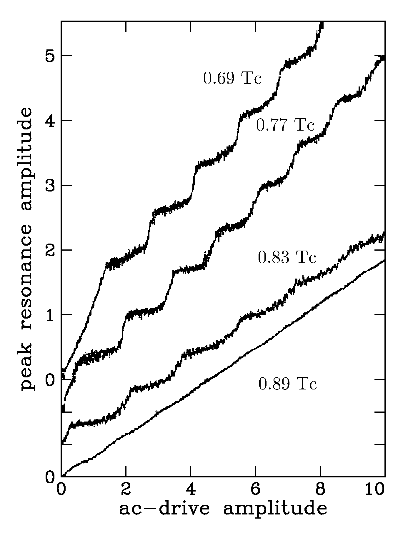
Figure 27: Staircase patterns (peak resonance amplitude versus applied drive level, both in arbitrary units) in ³He-B at a pressure of about 0.2 bar. The curves at various temperatures are shifted vertically for readability. Drive frequencies at the various temperatures are shifted from resonance so as to set comparable resonance conditions. From Avenel and Varoquaux (1988).

Expression (68) reduces in the limit $\Delta(T)/k_{\mathrm{B}}T\ll 1$ to the sinusoidal dependence of Eq.(64) for the current in terms of the phase difference across the barrier $\varphi_{\mathrm{b}}$. This result has been obtained by a number of authors using a variety of techniques. It is no real surprise that the details of the structure of the order parameter disappear when the dimensions of the orifice are small with respect to the coherence length and that s-wave-like results are found for both the A and B phases. Superfluid coherence is effectively weakened by the micro-orifice because the length over which it heals becomes larger than the physical size of the connecting duct; however, if the length of that duct is short enough, a sizeable supercurrent can still exist, sustained by the quantum tunnelling of quasi-particle pairs through the weak link.

At temperatures such that $\Delta(T)/k_{\mathrm{B}}T$ is no longer a small quantity, Eq.(68) becomes increasingly slanted with an abrupt slope close to $\varphi=\pi$ when ${\mathrm{cos}}\,\varphi/2$ changes sign while retaining the periodicity by $2\pi$ in the phase difference. It displays a discontinuity for $\varphi=\pi$ at $T=0$. This behaviour of the weak link comes on top of the effect of the hydraulic inductance of the Deaver-Pierce model: the CPR is bound to become hysteretic and multivalued even for an extremely small pinhole in the limit $T\longrightarrow 0$.

This simple theoretical description accounts well for the experiments of Avenel and Varoquaux (1988), whose results are reproduced in Fig.27. Similar findings have been reached by Backhaus et al. (1997) in an array of pinholes. Close to the superfluid transition, weakly-coupled reservoirs of superfluid ³He-B exhibit a behaviour that involves the direct analogues of both Josephson ac and dc effects in superconductors. The relation between the superfluid current and phase – or CPR – is well represented by a slanted sine function. In the range of applicability of Eq.(68), single micro-apertures and arrays behave alike. The existence in superfluids of the analogues of the Josephson effects in superconductors was thus established in 1988 on firm grounds, both experimentally and theoretically, but more features were soon revealed by further studies.

VII.4 Multivalued CPR’s, p states and p defects

While near-ideal Josephson behaviour prevails in ³He-B at low pressure close to $T_{\mathrm{c}}$, departures from a sinusoidal current-phase relation were observed by Avenel and Varoquaux (1988, 1989) in a single orifice and later by Backhaus et al. (1997); Marchenkov et al. (1999) in an array of 0.1$\mu$m–diameter apertures, evolving to a near-straight line relation below 0.6 $T_{\mathrm{c}}$. The latter case is reminiscent of the situation in ⁴He, in which vortices are nucleated.

As the temperature is lowered further below $T_{\mathrm{c}}$, the superfluid coherence length becomes smaller than the aperture size used in present-day experiments. This trend is even more pronounced at higher pressure, where $T_{\mathrm{c}}$ is higher (and $\xi_{0}$ smaller). Room is thus left for a wall dominated order parameter texture within the weak link or its immediate proximity: the p-wave nature of superfluid ³He can then reveal itself.

Very detailed numerical simulations based on the time-dependent Ginzburg-Landau equations have been carried out by Soininen et al. (1992) for a finite size aperture quite similar to the one used by Avenel and Varoquaux (1988). These simulations show in colourful figures the time evolution, when the ³He superfluid is set to flow through the micro-slit, of the components of the superfluid density tensor parallel to the two short dimensions of the slit. Both the mass and the spin degrees of freedom of the spin-triplet p-wave order parameter take part in the phase slippage process. The various components of the order parameter evolve separately in space and time and do not go to zero simultaneously at the same location in the micro-aperture. The regions of space, in which the order parameter is depressed and about which the phase slips, peel off from the walls and traverse the slit at right angle with the flow direction. Thus, phase slips in the p-wave superfluid exhibit a fairly complex spatial and temporal evolution both in the pseudo-isotropic B phase and in the anisotropic A phase. In addition, the A phase may sustain core-less phase slippage as suggested by Anderson and Toulouse (1977) and as discussed below. These simulations also illustrate the details of operation of a vortex mill (Soininen et al., 1992) in which phase slip avalanches and multiple vortex creation take place. The state of sophistication of

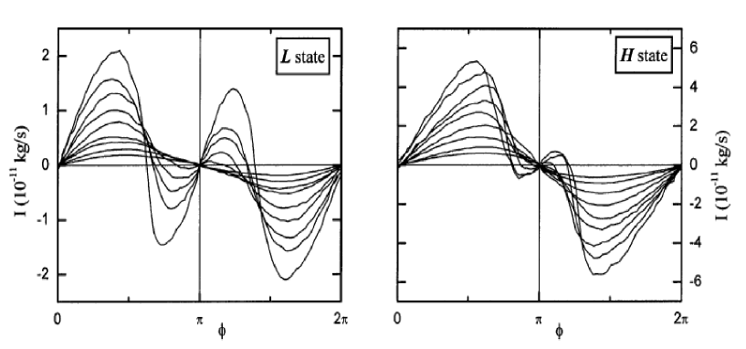
Figure 28: Current-phase relations in ³He-B observed in an array weak link. The two panels show CPR’s for the low current state (left panel) and the high current state (right panel) for temperatures ranging from $T/T_{\mathrm{c}}=0.850$ down to 0.450 $T/T_{\mathrm{c}}$ in steps of approximately 0.05$\,T/T_{\mathrm{c}}$. The mass current through the weak link increases as the temperature is lowered. At temperatures close to $T_{\mathrm{c}}$, the current-phase relations can be fit well with the Deaver-Pierce model. At the temperature decreases (and the critical current increases), this model becomes inadequate as a $\pi$-periodic component gradually sets in. From Marchenkov et al. (1999).

the microscopic description of superfluid ³He makes it possible to obtain such detailed information.

The phase slippage observations in superfluid ³He reflects this wealth of riches. While near-ideal Josephson behaviour prevails in ³He-B at low pressure close to $T_{\mathrm{c}}$, more complicated staircase patterns than those shown in Fig.(27) develop below $0.7T_{\mathrm{c}}$ (Avenel and Varoquaux, 1989), which cannot be described by the Deaver-Pierce model. These patterns are not even reproducible from one cool-down through $T_{\mathrm{c}}$, or through the A to B transition, to the next. It is likely that different order parameter textures and topological defects are coming into play.

Among those features, two notable ones were reported by Backhaus et al. (1998); Marchenkov et al. (1999) and are shown in Fig.28 in ³He-B at saturated vapour pressure. These authors used a two-hole micro-resonator with a weak link made of a 65x65 array of 100 nm round holes micro-machined in a 50 nm thick silicon nitride free-standing membrane. The 4225 holes in parallel offer a large enough flow path for the mass flow rate under an applied pressure head to be closely monitored. They operated the resonator in free ringing mode and recorded the transient response following a large impulsive drive excitation. The phase is derived from the measurement of the pressure head between the two sides of the weak link by integration of Eq.(14). The current-phase relations displayed in Fig.28 are obtained with this direct technique.

The first feature shown in Fig.(28) is the existence of two possible CPR’s at the same temperature, one with a larger critical current than the other, the second, the appearance in the $2\pi$-periodic CPR of an increasingly strong $\pi$-periodic admixture as the temperature is lowered. Avenel et al. (1998b) pointed out that this admixture could simply arise from the unavoidable dispersion between the sizes of the micro-holes in the array. This rather trivial explanation holds in part under all circumstances but is not the end of the story, as was soon shown by Avenel et al. (2000)’s own observations using a single micro-aperture for which there is obviously no scatter in critical currents or transit times.

Avenel et al. (2000) and Mukharsky et al. (2004) took advantage of the Sagnac effect (see §VIII.1) to ramp up and down in a precise manner the macroscopic phase difference $\delta\varphi$ applied across the weak link. They reported the observation of several different CPR branches – usually more than two – most with $\pi$-components and with different critical velocities at the same temperature but in different cooldowns through the superfluid transition temperature. Each of these several $J(\varphi)$’s was usually robustly fixed in each run and the general trend was to go from $2\pi$ periodicity to $\pi$ periodicity as the temperature is lowered, although, occasionally, no $\pi$ periodicity was observed even at the lowest temperature. At higher pressure (10 bars), hysteretic behaviour in the single micro-aperture was prevalent and up to three simultaneous branches for the CPR were observed. Switching between these different branches could be triggered by applying strong transient drive voltage to the resonator, indicating that textural effects were most likely at play.

Some of these features were actually predicted long before their observation by Thuneberg (1988) who worked out a numerical solution for the Ginzburg-Landau equations of the state of ³He-B confined inside a micro-aperture. This author found two different CPR’s according to whether the $\hat{\boldsymbol{\mathrm{n}}}$-vector of the B-phase order parameter, assumed to lie perpendicular to solid walls, is in a parallel or antiparallel configuration on both sides of the membrane carrying the micro-aperture. In the antiparallel configuration, the spin and mass currents are out of phase, resulting in a lower critical current. Eventually, the decoupling between mass and spin currents leads to the admixture of a $\pi$-periodic component to the 2$\pi$-periodic CPR.

The experimental discovery of these effects by Backhaus et al. (1998) and Marchenkov et al. (1999) spurred theoretical interest. Thuneberg’s numerical findings were soon confirmed and sharpened by the analytic investigations of Yip (1999) and Viljas and Thuneberg (1999, 2002b) and extended numerical simulations for two-dimensional geometries by Viljas and Thuneberg (2002a). The upshots of these studies are the following:

• $\bullet$ Following Yip (1999) and Viljas and Thuneberg (1999), the $\pi$ states in ³He-B are due to the interference of currents carried by quasiparticles with different spins that acquire different excess phases from the internal spin structure of the order parameter while travelling through the weak link. More specifically, the $\ket{\uparrow\uparrow}$ and $\ket{\downarrow\downarrow}$ Cooper pair populations may be viewed as independent superfluids, the phases of which may be slightly shifted with respect to one another because of a differing spin-orbit coupling. Summing the corresponding mass currents, given by Eq.(68), represented by slanted sine CPR’s shifted in phase by $\pm\delta\varphi$ leads, if the shift is large enough, to a positive-slope branch in the CPR at $\pi$: this $\pi$-state mechanism relies on different spin-orbit orientations on both sides of the weak link and operates at the single pinhole level (Viljas and Thuneberg, 2002a).

• $\bullet$  The Josephson coupling between two baths of ³He-B mixes the phase difference to the spin-orbit texture of the order parameter: the equilibrium configuration of the texture then depends on the phase bias applied to (hence on the current carried by) the weak link. The texture is assumed fixed in the simpler calculations: this is the isotextural case, which offers only a coarse agreement with observations. If the texture is allowed to adjust to the local mass and spin currents by expressing the balance between its stiffness and its interactions with the walls and with the mass current, a $\pi$-state can also arise: this anisotextural effect requires a self-adjusting string of calculations and provides quantitative agreement with pinhole array experiments (Viljas and Thuneberg, 2002b).

• $\bullet$ These refined calculations led to the realisation that multiple Andreev reflections and sub-gap structures also played a role in the transmission of the supercurrent through the weak link Asano (2001), and that a A-like phase inside the superfluid junction could also result in the existence of a $\pi$-state (Nishida et al., 2002).

• $\bullet$ Dissipation in pressure-driven dc-supercurrents (Simmonds et al., 2000) could also be explained by multiple Andreev reflections (Mukharsky, 2004; Viljas, 2005) or by time-dependent anisotextural effects and spin-wave emission, (Viljas and Thuneberg, 2004a; Viljas, 2005): if a pressure difference is applied across the weak link, an ac-oscillation (at the ac-Josephson frequency) of the texture ensues, causing dissipation by spin-wave radiation. The two dissipation mechanisms, sub-gap processes and textural losses, can come on top of one another.

Observations related to these topics are those of Mukharsky et al. (2004) who, in the course of high-precision CPR measurements using the Sagnac effect described in §VIII.1, found the signature of a stable textural defect that sustains a change of the phase by $\pi$ away from the weak link. This differs from the $\pi$-state discussed above. “Cosmic-like” solitons, proposed by Salomaa and Volovik (1988), could constitute such a defect but they are thought to be unstable in the bulk of the superfluid.

A comprehensive study of the possible planar interfaces between two domains of superfluid ³He-B has been conducted by Silveri et al. (2014). Of all the possible planar structures allowed by the symmetries of the B-phase order parameter, only one is found to be energetically stable in the presence of walls. This particular interface is characterised by the vanishing of one of the components of the interfacial order parameter along a gap-node direction contained in the plane of the domain wall. It sustains a phase change by $\pi$ and can appear as a remnant of the A to B interface during cool-down through the transition.

In the perspective of the present article (see also the review by Davis and Packard (2002)), these complex features of the Josephson supercurrents illustrate quite vividly the nature of the superfluid order parameter and of the phase coherence it entails. But their detailed studies are complicated because they are entangled with order parameter textures, as mentioned above, but also because the state of the superfluid inside the micro-junction may not be precisely accounted for, as discussed in the next Section.

VII.5 The peculiarities of the A-phase

The A-phase takes over from the B-phase at the superfluid transition temperature above a pressure of 21.2 bars. Strong coupling effects resulting from atomic localisation increase with density. Part of these enhanced interactions is mediated by spin-spin exchange, the so-called paramagnons. Because of these effects, the A-phase condensate only consists of $S_{\mathrm{z}}$ = +1 and -1 pairs, ($\ket{\uparrow\uparrow}$ and $\ket{\downarrow\downarrow}$), and the energy gap above the Fermi surface $|{\mathrm{\boldsymbol{\Delta}}}(\hat{\mathrm{\boldsymbol{k}}})|$ is strongly anisotropic while retaining the $L=1$ symmetry: it vanishes at a node in the direction of $\hat{\boldsymbol{\mathrm{l}}}$, the orbital quantisation axis. As for its spin part, the A-phase behaves in some respect as an antiferromagnet with a spin quantisation axis $\hat{\boldsymbol{\mathrm{d}}}$. Its stability with respect to the B-phase is enhanced by an external magnetic field.

The A-phase order parameter in zero magnetic field is expressed in terms of three unit vectors, the spin quantisation axis $\hat{\boldsymbol{\mathrm{d}}}$, and the orthonormal vectors $\hat{\boldsymbol{\mathrm{m}}}$ and $\hat{\boldsymbol{\mathrm{n}}}$ forming a triad with $\hat{\boldsymbol{\mathrm{l}}}$, the direction of the orbital angular momentum of the pairs. It is written in tensorial notation as:

$$A_{\mu i}=\Delta_{\mathrm{A}}\hat{d_{\mu}}(\hat{m_{i}}+\mathrm{i}\,\hat{n_{i}})\;.$$ (69)

In ⁴He, the Bose order parameter is a simple complex number and the phase comes in quite naturally as it does for the BCS order parameter in s-wave superconductors, for ultracold atoms, and for the B-phase order parameter, Eq.(67), as discussed above.

No single phase factor appears spontaneously in expression (69) for the A-phase order parameter. However, the single-particle wave function in the condensate still possesses an overall phase among other components. This phase goes over to the macroscopic Bose order parameter, which inherits of a global $U(1)$ phase rotation broken symmetry.

But this is not the whole story: a rotation of the triad $\hat{\boldsymbol{\mathrm{l}}},\,\hat{\boldsymbol{\mathrm{m}}},\,\hat{\boldsymbol{\mathrm{n}}}$ about the angular momentum directrix $\hat{\boldsymbol{\mathrm{l}}}$ by angle $\gamma$ also contributes an overall phase factor to the A-phase order parameter. This property can be seen readily by considering the complex plane perpendicular to $\hat{\boldsymbol{\mathrm{l}}}$ containing the complex vector $\hat{\boldsymbol{\mathrm{m}}}+\mathrm{i}\,\hat{\boldsymbol{\mathrm{n}}}$ that appears in Eq.(69): a rotation by angle $\gamma$ in the complex plane transforms $\hat{\boldsymbol{\mathrm{m}}}+\mathrm{i}\,\hat{\boldsymbol{\mathrm{n}}}$ into ${\mathrm{exp}}(-\mathrm{i}\gamma)\,(\hat{\boldsymbol{\mathrm{m}}}+\mathrm{i}\,\hat{\boldsymbol{\mathrm{n}}})$. The Galilean invariance argument as used to derive the two-fluid model for ⁴He leads, when everything is told, to the following expression for the velocity of superfluid mass transport:

$${\mathbf{v}_{\mathrm{s}}}=-\,\frac{\hbar}{2m_{3}}\,(\nabla\gamma+\cos\beta\,\nabla\alpha)\;.$$ (70)

The Euler angles $\alpha,\beta,\gamma$ fix the orientation of the orbital triad $\hat{\boldsymbol{\mathrm{l}}},\,\hat{\boldsymbol{\mathrm{n}}},\,\hat{\boldsymbol{\mathrm{m}}}$ in the chosen reference frame, $\gamma$ expressing a rotation about $\hat{\boldsymbol{\mathrm{l}}}$ as already mentioned. Two independent phase gradients appear in Eq.(70). In one, $-\nabla\gamma$, the angle plays the role of the usual phase $\varphi$. This feature arises because the $U(1)$ phase rotation broken symmetry as already mentioned. The other stems from the bending of the $\hat{\boldsymbol{\mathrm{l}}}$-texture. Superflow is not simply governed by the gradient of the global phase alone. The velocity field $\boldsymbol{v_{\mathrm{s}}}$ is no longer irrotational in general, hence the circulation of $\boldsymbol{v}_{\mathrm{s}}$ over a closed loop is no longer necessarily quantised.

In the presence of non-uniform $\hat{\boldsymbol{\mathrm{l}}}$ textures, the change of orientation of $\hat{\boldsymbol{\mathrm{l}}}$ in space may also contribute to the supercurrent. The contour integral of Eq.(70) along a closed loop $\Gamma$ can be put under the form

$${\oint_{\Gamma}\,\boldsymbol{v}_{\mathrm{s}}\cdot\mathrm{d}\boldsymbol{r}=\frac{\hbar}{2m_{3}}\,\big{[}2\pi n+\sigma(\cal D}\big{]}\;.$$ (71)

The first contribution to the rhs of Eq.(71 is recognised as the quantised velocity circulation around line singularities, as found in superfluid ⁴He, the second is expressed (Ho, 1978) as the area circumscribed on the unit sphere by unit vector $\hat{\boldsymbol{\mathrm{l}}}$ when carrying the loop integral along contour $\Gamma$. This last contribution is nil in the trivial case

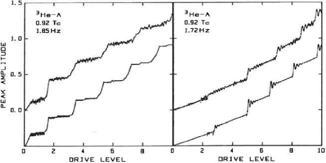
Figure 29: Staircase patterns in the A-phase at 28.4 bars and $T=0.92T_{\mathrm{c}}$ ($T_{\mathrm{c}}=2.417$ mK). The left and right panels show the patterns slightly above and below the resonator resonance at $\omega_{\mathrm{m}}=1.783$ Hz, as observed (upper curves) and as computed (lower curve) with the Deaver-Pierce model. From (Avenel and Varoquaux, 1989).

where $\hat{\boldsymbol{\mathrm{l}}}$ keeps pointing in a fixed direction. There exist other less-trivial cases with $\sigma({\cal D})=0$ as discussed by Ho (1978), but, in general, this contribution is non-zero and the velocity circulation is non-quantised.

The interplay between superflow, vortices and textures of the order parameter becomes quite complex. In particular, the A-phase persistent superflow can be relaxed by textural motion alone without the creation of topological singularities of the order parameter such as vortices. However, if large-scale motion of the texture is suppressed, dissipation can be quenched and persistent currents stabilised, as shown by the experiments of Gammel et al. (1985). The authors demonstrated the existence of such currents in the annular space of a torsional oscillator packed with 25 m  silicon carbide powder. The effect of the powder was to immobilise $\hat{\boldsymbol{\mathrm{l}}}$. The (small) supercurrent was detected indirectly through its effect on the damping of the small-amplitude of the torsional oscillator. This crafty experiment showed that the A-phase possesses, if to a less convincing extent than the B-phase, the distinctive attribute of dissipationless flow.

The phase slippage concept can also be extended to the A-phase, as proposed by Anderson and Toulouse (1977). Josephson-type experiments can be contemplated with some uncertainty as to their outcome because of the lack of quantisation of the velocity circulation, and also because of the large dissipation associated with the motion of the order parameter gap in the direction of $\hat{\boldsymbol{\mathrm{l}}}$, where its nodes lie.

These experiments were attempted by Avenel and Varoquaux (1989) with the same resonator as for their B-phase experiments. They did observe staircase patterns in the A-phase both close to the superfluid transition temperature with a rather non-ideal current-phase relation, and further down in temperature where new features occurred. The patterns shown in Fig.29 obtained in the A-phase at $T=0.92T_{\mathrm{c}}$ at frequencies slightly above and below the resonance frequency of the flexible wall resonator are quite well defined but differ markedly: they exhibit large dispersive effects, a sharply peaked resonance and low dissipation. The outcome of numerical simulations of the resonator response using the Deaver-Pierce model, Eq.(66) are shown below the experimental data curves. The resonance quality factor is high, $Q=80$. The non-ideality parameter $\alpha$ is equal to 5: the phase slips are hysteretic and weakly dissipative.

Given this observation that the A-phase phase-slip pattern seems to follow the ubiquitous Deaver-Pierce model at 0.92 $T_{\mathrm{c}}$, it could be expected to become more and more ideal when raising the temperature closer to $T_{\mathrm{c}}$. This trend could unfortunately not be ascertained in these experiments because the operating frequencies, which decrease as $\rho_{\mathrm{s}}/\rho$, become too low and the useful signal gets lost in the background $1/f$ mechanical noise of the detection device.

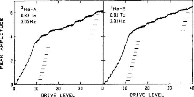
Figure 30: Staircase patterns in the A and B phases at nearly identical frequencies and temperature. The horizontal ticks mark the periodicity of the staircase pattern (top) and of the low-level structure (bottom). This low-level structure has been attributed by the authors to solid friction of unknown origin somewhere in the resonator (but may also arise from sub-gap energy levels). From (Avenel and Varoquaux, 1989).

Further down in temperature, an instructive direct comparison between the A-phase response and that of the B-phase at high pressure can be carried out by taking advantage of the following circumstance: at 28.4 bars, the A to B transition occurs at about 0.81 $T_{\mathrm{c}}$; it is signalled by a sudden drop in resonance frequency caused by the drop in superfluid density accompanying the first order transition. As the A-phase can be supercooled into the domain of stability of the B-phase, both phases can be studies at comparable frequencies.

The outcome of this comparison is shown in Fig.30 and reveals a remarkable similarity between the two phases. The response of the superfluid in the weak link depends little on whether the bulk of the liquid is in the A or the B phase. As discussed by Avenel and Varoquaux (1989), the observed behaviour inside the micro-slit corresponds well to the situation described by Kurkijärvi (1988) who finds that the current-phase relations for the A and B phases differ only little (see Eq.(68)). It may also happen that the state of the superfluid in the weak link remains the same irrespective of the state in the bulk. It has been predicted by Li and Ho (1988) and Fetter and Ullah (1988) that the A-polar phase would be favoured by the depletion of some of the components of the A-phase order parameter close to the aperture walls.

The sub-gap structure, shown in Fig.30, which develops for resonance amplitudes below the critical threshold at which dissipative phase slips start to occur, is quite intriguing. It is interpreted by Avenel and Varoquaux (1989) as arising from possible (aniso)-textural effects inducing solid friction. It could also possibly be revealing the existence of sub-gap resonant levels.

These experiments establish very clearly that phase slippage takes place in the A phase, that persistent currents can be trapped in the loop threading the double-hole resonator, and that the velocity circulation along these trapped currents changes by multiples of the quantum of circulation in the same manner as in the B phase: it so turns out, as was the case in the persistent current experiments by Gammel et al. (1985), that the $\hat{\boldsymbol{\mathrm{l}}}$-texture is sufficiently well pinned in the regions where ${\boldsymbol{v}_{\mathrm{s}}}$ picks up significant speed.

Topological defects, seen above to play an important role in phase slippage experiments, offer a vast and fascinating domain of study, both in the A and B phases. The vortex core develops complex structures, as reviewed by Salomaa and Volovik (1987). Vortex sheets can form in rotating ³He-A, as observed by Parts et al. (1994) using very sensitive NMR techniques, which have brought about a wealth of information on vortices in superfluids under rotation. This work has been reviewed by Finne et al. (2006). Analogies can be drawn between the formation of defects in superfluid ³He and that of cosmic strings in the Early Universe because the order parameter symmetries that can be broken are the same. These enticing prospects for experimental cosmology have been reviewed by Eltsov et al. (2000), Bäuerle et al. (2000), Bunkov (2010) and Volovik (2003) in his wonderful book. Phase slippage is beyond doubt relevant in these situations and will be used to study this vast new field.

VII.6 ⁴He close to the l–point

The existence of Josephson-like effects was thus clearly established in superfluid ³He for the dc-effect and in both ³He and ⁴He superfluids for the ac–effect by Year 2000. The remaining problem was the possible observation of a quasi-sinusoidal current-phase relation in ⁴He. The minuteness of the coherence length in ⁴He makes the fabrication of a suitable weak link a tall order except in the immediate vicinity of the l-point, where it diverges as $\xi=\xi_{0}(1-T/T_{\mbox{\footnotesize{l}}})^{-2/3}$ with $\xi_{0}\sim$ 1 to 2 Å  (Langer and Reppy, 1970). At the l-point however, superfluidity is suppressed by thermal fluctuations. Would the hydrodynamic Josephson effects not be even more readily washed out by the same token?

This concern was formalised by Zimmermann (1987) whose argument runs approximately as follows. The Josephson coupling energy is obtained from the Josephson current, Eq.(64), by integration with respect to $(\hbar/m_{\mathrm{4}})\mbox{\small{d}\hskip 0.19376pt}\varphi$. Its maximum value is therefore $(\hbar/m_{4})\,J_{\mathrm{c}}$ and reads

$$E_{\mathrm{J}}=\left(\frac{\hbar}{m_{4}}\right)^{2}\,\frac{s_{\mathrm{b}}}{b_{\mathrm{b}}}\,\frac{\rho_{\mathrm{s}}}{\sinh(l_{\mathrm{b}}/b_{\mathrm{b}})}\;.$$ (72)

In the weak coupling limit for which Eq.(64) holds, the wavefunction is strongly depleted within the barrier and the penetration length is smaller than the length of the barrier, $b_{\mathrm{b}}\lesssim l_{\mathrm{b}}$. Making use of the scaling relation between $\rho_{\mathrm{s}}(T)$ and $\xi(T)$ (Josephson, 1966),

$$\rho_{\mathrm{s}}\xi=(m_{4}/\hbar)^{2}k_{\mathrm{B}}T\;,$$ (73)

and since $\sinh(l_{\mathrm{b}}/b_{\mathrm{b}})>l_{\mathrm{b}}/b_{\mathrm{b}}$ it stems from Eq.(72) that

$$E_{\mathrm{J}}\lesssim\frac{s_{\mathrm{b}}}{l_{\mathrm{b}}}\,\frac{k_{\mathrm{B}}T}{\xi(T)}\;.$$ (74)

For the round pinhole with diameter $d$ considered by Zimmermann, $s_{\mathrm{b}}=\pi d^{2}/4$ and $l_{\mathrm{b}}>\ell_{\mathrm{h}}$, the hydraulic length $\ell_{\mathrm{h}}$ being $\pi d/4$ for a circular orifice, so that $E_{\mathrm{J}}<k_{\mathrm{B}}T\,d/\xi(T)$. Zimmermann concludes from this upper bound for the Josephson energy that, as $\xi(T)$ diverges upon approaching $T_{\mathrm{\mbox{\footnotesize{l}}}}$ from below, the Josephson coupling energy will end up being less than the thermal energy and that the Josephson dc-effect will be washed out by thermal fluctuations.

Similar concerns were spelled out by Ullah and Fetter (1989) for their calculations of weak link properties in ³He-B in the Ginzburg-Landau regime: “We do not address the important problem of thermal fluctuations destroying the superfluidity in the very small volume of the weak link. To our knowledge, there is no reliable, quantitative theory of the stability of the superfluid phase is severely confined geometries. We believe that this question can be convincingly answered only by experiment”. This remark is even more relevant to superfluid ⁴He close to $T_{\mbox{\footnotesize{l}}}$.

The first hint of a successful experimental observation was reported by Sukhatme et al. (2001). These authors used an array weak link of 24 micro-slits 3 mm x 0.17 mm about 10 mm apart in a 0.15 mm thick membrane. Their findings are summarised in Fig.31. At 3.72 mK below $T_{\mbox{\footnotesize{l}}}$ – the bottom curve in the figure, the scale of which is shrunk – the critical velocity is well-marked, as well as the staircase steps, indicating a dissipative phase slippage process. A phase-slip regime has been reached. This was hoped for since the temperature-dependent coherent length 3.72 mK below $T_{\mbox{\footnotesize{l}}}$, $\xi(T)=24$ nm, is smaller than the micro-slit width, but by less than one order of magnitude.

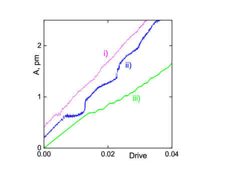
Figure 31: (Color online) Staircase patterns in ⁴He close to $T_{\mathrm{\mbox{\footnotesize{l}}}}$ (amplitude, in picometres versus drive, in arbitrary units, from Sukhatme et al. (2001)) for $T_{\mbox{\footnotesize{l}}}-T=$ 61 $\mu$K – curve i), 154 $\mu$K – curve ii), and 3.72 mK – curve iii). The plots are shifted vertically by 2 pm with respect to one another for clarity. The data for curve iii) has been divided by 20 along the $x$-axis and by 10 along the $y$-axis. As in the case of ³He-B – shown in Fig.27 – the height of the first step corresponds to the critical current $J_{\mathrm{c}}$. Each subsequent step corresponds to an additional phase difference of $2\pi$ (Courtesy of Yuri Mukharsky).

Getting closer to $T_{\mbox{\footnotesize{l}}}$ from below, successively at $T_{\mbox{\footnotesize{l}}}-T=154$mK, and 61 mK, the expected trend toward a smoother, less dissipative staircase pattern is observed, much like in Fig.(27) for ³He, supporting the conclusion that the same hydrodynamic ideal Josephson effect can be observed in superfluid ⁴He close to the superfluid transition temperature $T_{\mbox{\footnotesize{l}}}=2.17$ K.

This conclusion raises questions, and possibly, some eyebrows as well:

• $\bullet$  Would, for some reason, Zimmermann’s argument be invalid?

• $\bullet$  How come that dissipative phase slippage, the mechanism for which seems to rely on the nucleation of a single vortex and its crossing of all streamlines of the superfluid flow through a single micro-slit also operates for an extended array of them?

Zimmermann’s original argument, outlined above, was applied to a single round hole. Sukhatme et al. (2001)’s 24 parallel slits yield an estimated enhancement factor of 500 in the superflow passage area $s_{\mathrm{b}}$ that appears in Eq.(74), provided that the supercurrents in the apertures effectively sum up. The overall Josephson energy is increased by the same factor and the disruptive effect of thermal fluctuations is pushed back much closer to $T_{\mbox{\footnotesize{l}}}$. This line of reasoning was pursued by Chui et al. (2003), but its soundness depends on the answer to the second question, which turns out to be trickier.

The Berkeley group carried out a number of studies with aperture arrays similar to those used for ³He-B by Marchenkov et al. (1999). The size of the round pinholes in these arrays, 90 nm in diameter, is comparable to the coherence length one millikelvin away from the l-point but the distance separating the pinholes, located on a 3 mm square lattice, is much larger. Two phase-slippage regimes are identified when the temperature is lowered below $T_{\mathrm{\mbox{\footnotesize{l}}}}$ as already reported by Sukhatme et al. (2001). At $\sim$ 50 to 100 mK below $T_{\mathrm{\mbox{\footnotesize{l}}}}$ (and slightly further down in temperature in the experiments by Sato et al. (2006)), a reversible (non-dissipative) Josephson regime is observed. In this regime, the phase-slips occur in a fully synchronous manner. Between approximately 0.3 to 15 mK below $T_{\mathrm{\mbox{\footnotesize{l}}}}$, a transition toward a dissipative phase-slip regime sets in as the synchronisation between the apertures gets lost. Further below $T_{\mathrm{\mbox{\footnotesize{l}}}}$, the phase-slip regime becomes asynchronous. The amplitude of the resultant phase slippage signal from the array does not sum up to what it should be. It also exhibits large slips and collapses somewhat similar to those described in §VI.2 for a single orifice (but of a different sort, see below).

It is clear that inhomogeneities in aperture size and surface properties, the edge effects at the periphery of the array, and local critical fluctuations introduce a spread in the values of the critical current in the different apertures. Phase slips occur at different times during resonator motion. The summation of the currents through the various apertures, as attempted in the numerical simulations of arrays of superfluid Josephson junctions by Avenel et al. (1998b), Pekker et al. (2007), and Sato et al. (2007) has to be exercised with care.

It can be argued (Chui et al., 2003) that the Josephson currents in the micro-apertures are small and perturb little the quantum phases in the bulk on both sides of the membrane supporting the weak link array. Phases are well defined below $T_{\mathrm{\mbox{\footnotesize{l}}}}$ – for instance, the quantisation of circulation is enforced – and so should their difference. This reasoning would appear to leave only one degree of freedom to undergo fluctuations, with a thermal energy of $k_{\mathrm{B}}\,T/2$ to be shared among the $N$ apertures of the array: the effect of fluctuations in each individual aperture would effectively be quenched on taking the average over the whole array.

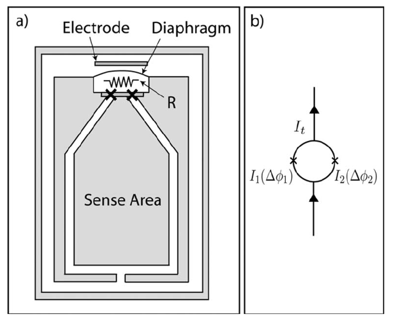
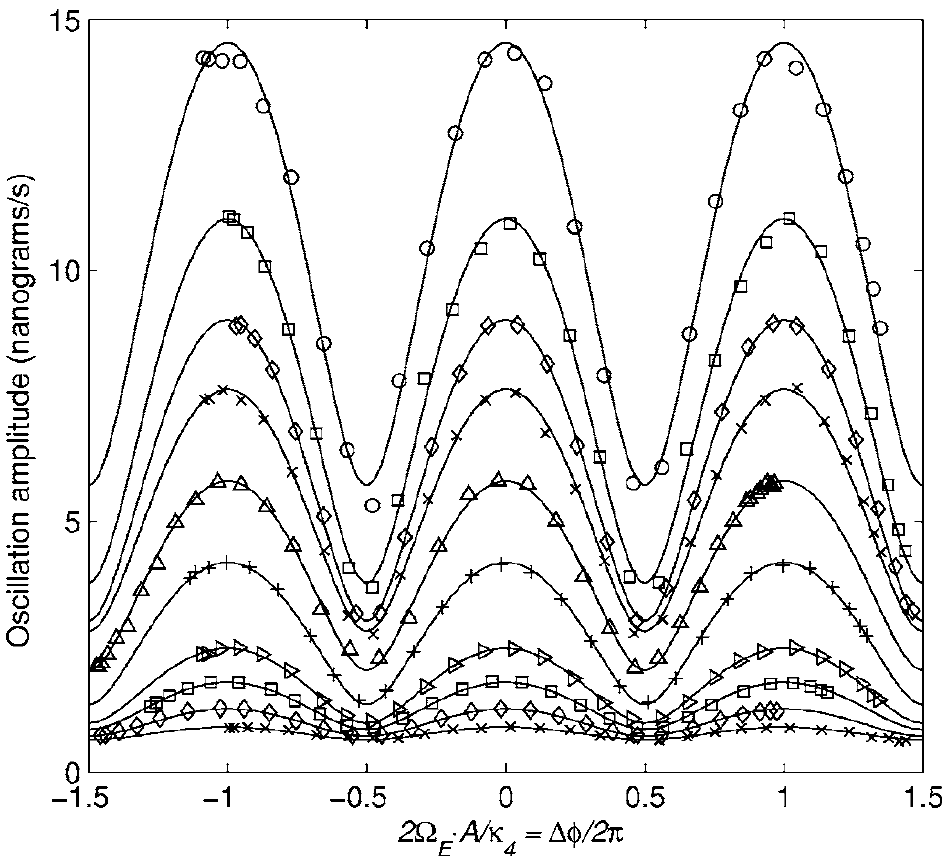
Figure 32: Superfluid Interferences in a two-aperture resonator.
Top panel: (a) Sketch of the hydromechanical resonator. The unshaded regions are filled with superfluid ⁴He. The flexible metallised diaphragm at the top of the upper chamber serves both as a microphone to detect the resonant oscillations and as a pressure pump to drive the flow across the two aperture arrays indicated by crosses. These arrays interrupt the superfluid channel enclosing the sense area. (b) Diagram of the resonator equivalent circuit showing the analogy with the electrodynamic dc-SQUID. There are two superposed currents flowing through the weak links, one corresponding to the rotation flux picked-up by the sensing loop, Eq.(76), the other being the common-mode read-out current from the flexible diaphragm.
Bottom panel: Peak amplitude of the diaphragm displacement on resonance as a function of the rotation flux $2\,{\bf\Omega}\cdot{\bf A}$ picked up by the superfluid loop enclosing the sense area – see §VIII.1 for a detailed description of these interferometer operation based on the Sagnac effect. The measured data is shown by the symbols; the solid lines are fits to the data of the equation modelling the resonator motion as described by Hoskinson et al. (2006b). The modulation curves were taken at temperatures $T_{\mbox{\footnotesize{l}}}\,-\,T=$ 12, 7.0, 4.0, 3.0, 2.0, 1.5, 0.9, 0.6, 0.4, and 0.3 mK from top to bottom. This temperature span covers the coherent Josephson regime in the array discussed in §VII.6. From Hoskinson et al. (2006b)

This argument has to be stretched a long way to explain the large span in $T_{\mbox{\footnotesize{l}}}-T$ over which the synchronous phase-slippage regime subsides both very close to the l-point when quantum coherence should end up being killed by thermal fluctuations, and quite a way below it where it should be randomised by array imperfections. In other words, the robustness of the coherence effect mentioned above against dephasing by environmental effects appears quite remarkable. Perron et al. (2013) have pointed out that the superfluid onset in the micro-slits used by Sukhatme et al. (2001) is expected to be depressed by size effects to $T_{\mbox{\footnotesize{l}}}-T_{\mathrm{c}}\simeq 430$ mK whereas the Josephson effect could be tracked to as close as 28 mK below $T_{\mbox{\footnotesize{l}}}$. Similarly, for the pinholes used by Sato et al. (2006), $T_{\mbox{\footnotesize{l}}}-T_{\mathrm{c}}\simeq 2.3$ mK while the Josephson effect survived up to possibly 0.5 mK from $T_{\mbox{\footnotesize{l}}}$. As concluded by Perron et al. (2013), “in both experiments one obtains superflow in a temperature region where the helium in the isolated weak links should be normal. Both of these experiments are thus relying on proximity effects, due to the surrounding bulk liquid, to maintain a non-zero order parameter in the weak links”.

These authors draw their conclusion from studies of the interconnection of an array of 2 mm$\times$2 mm micro-pools linked through the film of superfluid ⁴He. They have found from measurements of the specific heat and the superfluid fraction in the vicinity of $T_{\mbox{\footnotesize{l}}}$ that correlation effects are still effective at distances up to 100 times $\xi(T,L)$, the finite-size correlation length suitably renormalised for confinement over the distance $L$, the size of the micro-pools boxes. The unexpectedly large extent of the correlation observed between micro-pools can be likened to the robustness of the coherent behaviour of Josephson junction arrays close to $T_{\mbox{\footnotesize{l}}}$.

Pekker et al. (2007), besides their numerical studies referred to above, also treated the problem of aperture current summation in an irregular array as an order-disorder transition in a mean-field approximation approach. They introduce a distribution of aperture critical currents and an effective inter-aperture coupling parameter. They report qualitative agreement with the experiments of Sato et al. (2006) including “system-wide avalanches”, both in the numerical simulations of the array behaviour and in the ordering transition approach.

The observed long range of cross-aperture coupling may arise from a simple classical hydrodynamics scheme, which is an extension to arrays of the putative mechanism for single-aperture large slips discussed in §VI.2. Suppose that, during the surge of the superflow through the array, a (quantum) phase slip occurs early in one of the apertures, releasing a vortex half-ring that starts drifting (classically) sideways along the membrane supporting the array. Soon, this vortex half-ring runs into the flow lines emerging from a nearby aperture, gaining energy from it to proceed in its course and, possibly, triggering the nucleation of another vortex half-ring, and so on. This multiplication process may die by itself at the ebb of the flow. Or, if it overcomes the friction on the normal component, it may trigger $2\pi$ slips over all the microholes of the array, or, possibly, swell to the system-wide avalanches (Pekker et al., 2007) observed by Sato et al. (2006). This mechanism for avalanches are thus intrinsic to aperture array dynamics and distinct from flow collapses in single apertures discussed in §VI.2.

Even more so than in single apertures, “macroscopic quantum coherence” manifests itself in the aperture array in a dual manner. First, the condensate acts as an ideal Euler fluid, maintaining orderly streamlines throughout the superflow in accordance to the Kelvin-Helmholtz theorem. Then, when a non-adiabatic process takes place, violating velocity circulation conservation, it does so in a quantum manner, allowing the phase to change by multiples of $2\pi$, for instance by the nucleation of a quantised vortex or by the current source or sink provided by Josephson tunnelling through a thin barrier of normal fluid.

VIII Concluding comments

VIII.1 Matter waves and superfluid interferometry

The single-hole or two-hole hydromechanical resonators used in the phase slippage experiments described above have been presented so far as the analogues of rf or dc superconducting quantum devices (SQUIDs), a useful analogy to help understand the way they operate. Another analogy is used in this Section to illustrate the concept of coherent matter fields, or matter waves, introduced for superfluid helium by Anderson in 1965. These devices are now considered as the likes of optical Sagnac interferometers; as the latter, they can be used to measure absolute rotations with very high sensitivity.

Consider a pool of superfluid in the shape of a conduit bending on itself as shown in Figs.32 or 34. The circulation of the velocity is quantised in the inertial frame – the reference frame fixed with respect to the distant stars – along any closed contour $\Gamma$ located entirely in the superfluid:

$$\oint_{\Gamma}{\bf v}_{\mathrm{s}}\cdot{\mathrm{d}}{\bf l}=\frac{\hbar}{m_{\mathrm{a}}}\,\oint_{\Gamma}\,\nabla\varphi\cdot{\mathrm{d}}{\bf l}=n\kappa_{\mathrm{a}}\;,$$

where $\kappa_{\mathrm{a}}=2\pi\hbar/2m_{3}$ for ³He, 3/2 times that quantity for ⁴He, and $n$ is an integer.

If the cryostat housing the pool is set into rotation with rotation vector ${\bf\Omega}$, the velocity transforms in the new frame according to ${\bf v}^{\prime}_{\mathrm{s}}={\bf v}_{\mathrm{s}}-{\bf\Omega}\times{\bf r}$ and the quantisation of circulation condition now reads

$$\oint_{\Gamma}{\bf v}^{\prime}_{\mathrm{s}}\cdot{\mathrm{d}}{\bf l}=n\kappa_{\mathrm{a}}-\oint_{\Gamma}{\bf\Omega}\times{\bf r}\cdot{\mathrm{d}}{\bf l}=n\kappa_{\mathrm{a}}-2\,{\bf\Omega}\cdot{\bf S}_{\Gamma}\,,$$ (75)

${\bf S}_{\Gamma}$ being the geometrical (oriented) area of the closed superfluid contour.

For an actual conduit with finite cross section such as the one pictured in Figs.32 and 34, there is a variety of choices for the contour $\Gamma$. The mean circulation of the velocity results from a suitable average over the various distinct superfluid contours threading the conduit. Taking the average of Eq.(75) over all the streamlines threading the conduit amidst stray thermal currents, pinned vortices, and textures, weighed according to the (infinitesimal) mass current that they carry, leads to (Avenel et al., 1997):

$$\left\langle\oint_{\Gamma}{\bf v}^{\prime}_{s}\cdot{\mathrm{d}}{\bf l}\right\rangle=n\kappa_{\mathrm{a}}+\kappa_{\mathrm{b}}-2\,{\bf\Omega}\cdot{\left\langle\bf S\right\rangle}\,,$$ (76)

where $\left\langle{\bf S}\right\rangle$ is the average of the contour areas over the conduit. The average of the quanta of circulation carried by the various streamlines, $\left\langle n\right\rangle\,\kappa_{\mathrm{a}}$ has been written as $n\,\kappa_{\mathrm{a}}+\kappa_{\mathrm{b}}$ to explicitly separate the non-quantised phase bias $\delta\varphi_{\mathrm{b}}=2\pi\kappa_{\mathrm{b}}/\kappa_{\mathrm{a}}$ arising from pinned vorticity from the strictly quantised contribution $2\pi n$.

The last term to the right of Eq. (76) also amounts to a non-quantised contribution to the phase bias, which varies with the flux of the rotation vector ${\bf\Omega}$ through $\left\langle\bf S\right\rangle$: the measurement of the corresponding phase difference with the interferometers depicted in Figs.32 or 34, $\delta\varphi_{\mathrm{S}}=(m_{\mathrm{a}}/\hbar)\,2\,{\bf{\Omega\cdot\left\langle S\right\rangle}}$, gives access to the rotation velocity. Alternatively, changing the orientation with respect to the North axis of the superfluid loop picks up more or less of the rotation flux due to the Earth rotation $\Omega_{\oplus}$. A known phase difference can be coupled to the weak link. The experimenter is provided with a “gauge wheel” to steer the phase.

Exploiting the properties of superfluids to detect very slow rotations has been proposed even before the discovery of the Josephson effects in superfluids, understandably with some lack of accuracy as to how the experiment could be conducted. Cerdonio and Vitale clarified in 1984 the way in which inertial and gravitational fields could be detected with superfluid ⁴He analogues of the rf-SQUID Cerdonio and Vitale (1984); Bonaldi et al. (1990). A number of authors followed suit afterwards for superfluid ³He and ⁴He Varoquaux et al. (1992); Packard and Vitale (1992); Hess (1992), and for the Bose-Einstein condensed gases Stringari (2001).

Detailed schemes for the actual implementation of superfluid ⁴He gyros have been worked out with the help of numerical simulations Avenel et al. (1994) and from the analysis of the operation of existing double-hole hydromechanical resonators. The first measurement of $\Omega_{\oplus}$ with a superfluid device was performed using a resonator operating in hysteretic mode in superfluid ⁴He with a rotation-sensing loop of 4.0 cm² by Avenel and Varoquaux (1996). Soon after, the Berkeley group reported the observation of the effect of the rotation of the Earth with a similar device operated in the staircase mode, in much the same way as conventional rf-SQUID magnetometers.

Figure 33: (Color online) Schematics of the optical Sagnac interferometer. A collimated beam from the source enters the interferometer through a beam splitter and is separated into two beams travelling along the optical path defined by the three mirrors in opposite directions, as indicated by the arrows. Re-entering the beam splitter, they recombine and produce a fringe pattern on the detector plate.

One may mention for the record that early attempts to measure $\Omega_{\oplus}$ led to disappointing results to the dismay of experimenters (Schwab et al., 1996a, b; Avenel et al., 1998a). It was however quickly realised that the currents in the bulk of the cell outside the resonator Avenel et al. (1998a); Schwab et al. (1998), simply caused by the re-orientation of the cryostat, were interfering with, and possibly overwhelming, the relatively weak $\Omega_{\oplus}$–induced Sagnac current in the pick-up loop. The influence of these stray currents can be made negligible by a proper design of the cell. A sheath on the port connecting the resonator to the main body of the cell was used to that effect by Avenel and Varoquaux (1996)(Avenel et al., 1997). The absence of such a decoupling device between the Sagnac current in the pick-up loop and the stray currents around the cell could cause uncontrolled inaccuracies of several tens of % (Schwab et al., 1996a, 1997, 1998).

The potentialities of superfluid gyros as extremely sensitive and stable rotation sensors, able to track, e.g., General Relativity effects, have been considered by Avenel et al. (1998a), Chui and Penanen (2005), Sato and Packard (2012) and Sato (2014). It appears that these gyros can compete with the most advanced rotation sensors, in particular because they are inherently driftless at very low temperatures.

These gyrometric devices are the direct superfluid analogues of the well-known Sagnac optical interferometers, as can be seen by inspection of the sketches of the latter in Fig.33 and of the superfluid device in Fig.34: the light source provides the incident light beam, the flexible membrane the supercurrent; counter-rotating waves travel along the square optical path, and along the coiled capillary, for the co-rotating part; the waves interfere in the beam splitter in the optical case, in the Josephson weak link in the superfluid case. The interferometer shown in Fig.32 is closer to a Mach-Zehnder interferometer than to a Sagnac one but the analogy goes along in the same way.

But is this reasoning by analogy, or the display of clear fringe patterns such as those shown in Fig.32, sufficient proof that the Sagnac effect is involved in the operation of these superfluid interferometers?

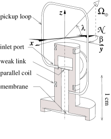
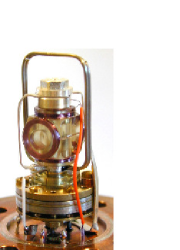
Figure 34: (Color online) Photograph and schematic view of the cell of Avenel et al. (2004), approximately to scale for the inner parts, except for the loop, which is made of two turns of 0.4 mm internal diameter capillary (only one turn is shown) with total area $5.90\,\pm\,0.10$ cm². The lower chamber of the resonator is a cylindrical duct, 1 mm in diameter, and connects the weak link to the flexible diaphragm (at the bottom) and to one end of the pickup loop (on the side); the upper chamber, a squat cylinder, is connected to the other end of the loop and to an inlet toward the main superfluid bath in which the resonator is immersed. Two pairs of coils produce fields parallel and perpendicular to the flow through the weak link to control locally the order parameter texture in ³He. The cryostat is rotated about the vertical axis $z$ by angle $\beta$ from the North, shown by a compass needle; $\lambda$ is the latitude, 48^∘43^′ at Saclay. This cell has been used to detect the rotation of the Earth from a “blind” laboratory with a sensitivity of $5\times 10^{-3}\,\Omega_{\oplus}\mbox{ Hz}^{-1/2}$.

Apparently not; superfluid gyros are still sometimes mistaken for purely inertial devices such as spinning tops, as discussed by Varoquaux and Varoquaux (2008). Clearly, the superfluid in a rotating bucket experiment is a dense medium. It can be weighed on a scale. For large enough rotation velocities, when enough vortex lines have been created, the fluid free surface eventually becomes concave, as in Newton’s rotating water bucket experiment. For small velocities however, things are different: the superfluid does not even starts spinning because of the absence of viscosity. Hence the common sense reluctance to admit that the far-fetched analogy between the behaviour of this condensed matter system and that of massless photons travelling at the velocity of light, or elementary particles like electrons or neutrons, or even confined ultra-cold atomic gases, holds any water.

A more formal approach is the following. As mentioned above, the Sagnac effect has been observed in a number of different physical systems, ranging from photon, electron, neutron and cold atomic gas interferometers to atomic clocks and the Global Positioning System. The unifying concept behind these widely different situations is provided by the transportation of Einstein clocks from location A to location B on a rotating platform (Langevin, 1921; Rizzi and Ruggiero, 2004).

Consider how these clocks can be synchronised, first when they are infinitely close to one another. The space-time metric is characterised in the conventional notation by $-\mathrm{d}s^{2}=g_{00}\mathrm{d}(x^{0})^{2}+2g_{0i}\mathrm{d}x^{0}\mathrm{d}x^{i}+g_{ii}\mathrm{d}(x^{i})^{2}$. The infinitesimal time interval $\mathrm{d}t$ between two nearly simultaneous events taking place at this given location in space is such that $\mathrm{d}s^{2}=g_{00}\mathrm{d}(x^{0})^{2}=-\mathrm{c}^{2}\mathrm{d}t^{2}$, $\mathrm{c}$ being the velocity of light.

If the clocks are now separated in space by an infinitesimal amount $\mathrm{d}x^{i}$ and the two events taken, say at location A, as the ticking of clock A for one and as the signal transmitted by clock B of its ticking a small distance away for the second, the two ticks occur with a time lag given by $\mathrm{c}\mathrm{d}t=-g_{0i}\mathrm{d}x^{i}\,/\,g_{00}\;,$ the repeated summation being on the space coordinates.

If clock B is now transported over a finite path $\Gamma$ closing on itself in a frame rotating with velocity $\mathbf{\Omega}$, the total time shift results from an integration along path $\Gamma$:

$$\Delta t=\frac{1}{\mathrm{c}}\,\oint_{\Gamma}\frac{g_{0i}\mathrm{d}x^{i}}{-g_{00}}=\oint_{\Gamma}\frac{\mathbf{\Omega}\!\boldsymbol{\times}\!\mathbf{r}\boldsymbol{\cdot}\mathrm{d}\mathbf{r}}{\mathrm{c}^{2}-(\mathbf{\Omega}\!\boldsymbol{\times}\!\mathbf{r})^{2}}\simeq\frac{2}{\mathrm{c}^{2}}\,\mathbf{\Omega}\boldsymbol{\cdot}\mathbf{S}\;,$$ (77)

$\mathbf{S}$ being the vector area subtended by the loop $\Gamma$.

Time delay (77) between the reading of the clock standing still on the rotating platform and that of the transported clock lies at the root of the Sagnac effect. As it depends on the rotation velocity and the actual path $\mathit{\Gamma}$, absolute clock synchronisation cannot be achieved. Sagnac corrections, Eq.(77), must be performed as done routinely for Global Positioning Systems (Ashby, 2004).

So much with clocks. For helium, a Lorentz invariant two-fluid model can be built over the usual Landau superfluid hydrodynamics as done by Carter and Khalatnikov (1992). The invariant velocity circulation, the generalisation of Eq.(16), reads

$$\int_{\Xi}\{v^{\prime}_{0}\mathrm{d}x^{0}+v^{\prime}_{i}\mathrm{d}x^{i}\}=n\kappa\;,$$ (78)

where $(v^{\prime}_{o},v^{\prime}_{i})$ is the four-velocity in the rotating frame $(c^{2}+\mathbf{v}^{\prime}_{\mathrm{n}}\boldsymbol{\cdot}\mathbf{v}^{\prime}_{\mathrm{s}}\,,-\mathbf{v}^{\prime}_{\mathrm{s}})$. The normal fluid velocity $v^{\prime}_{\mathrm{n}}$ and the superfluid velocity $v^{\prime}_{\mathrm{s}}$ are very small compared to $\mathrm{c}$ so that the time-like component of the four-velocity reduces to $\mathrm{c}^{2}$. The integration over $\Xi$ is an actual loop integral only for the space-like components. The corresponding world line is not closed because the time for synchronised clocks varies according to Eq.(77). Upon integration, Eq.(75) is recovered,

$$\oint_{\Gamma}v^{\prime}_{i}\mathrm{d}x^{i}=n\kappa+\int\!c^{2}g_{0i}\mathrm{d}x^{i}/g_{00}\simeq n\kappa-2\,\mathbf{\Omega}\boldsymbol{\cdot}\mathbf{S}\;,$$ (79)

which establishes the link between superfluid physics and the relativistic clock approach: the true and honest Sagnac effect described by the transported clocks, Eq.(77), and the circulation quantisation condition in the rotating frame leading to Eq.(76) are one and the same.

Thus, Einstein-synchronised clocks provide the time standard by which phase differences can be kept track of in all the studied physical systems. As appropriately summarised by Greenberger (1983) for neutron interferometry experiments: “the phase shift (in the rotating interferometer) is seen to be caused by the different rates at which a clock ticks along each of the two beams”. The rate at which that clock ticks for helium depends on the chemical potential $\mu$, due to the molecular field of the condensate as shown by Beliaev, and on the Sagnac phase shift.

The helium Sagnac experiments illustrate convincingly the reality of matter wave interference in the superfluid heliums, a substantially massive coherent field. Coherent, as shown at some length here, means coherence of the quantum phase, giving a wave-like character to a bulky fluid. A few remarks on this follow in a manner of conclusion.

VIII.2 Landau’s two fluids, ODLRO, and macrorealism

Anderson’s introductory words to the reprint of his 1966 paper in his book of 1994 are the following  :“I feel this is the clearest discussion of superfluidity available. Note that on many points this is contradictory or orthogonal to Landau orthodoxy as pronounced by Khalatnikov. Whether Landau would have agreed was never clarified because of his accident”. This remark poses the problem of the complementarity between the two-fluid model, the description of Bose condensation by the non-vanishing off-diagonal terms of the density matrix over a long range, and the macroscopic wavefunction approach.

Two crucial aspects of Landau’s legacy have been invoked here. The two-fluid model has ruled once and for good on the separation between normal fluid and superfluid components, both for the thermodynamics and the hydrodynamics. As used in this review in its reduced form for incompressible flows, which treats both components as independent, it has allowed to basically disregard the normal component. There are obviously limits to this high-handed simplification, especially close to the l-point, but it has provided the backbone of the simplified vortex dynamics of Sec.II and subsequent Sections on phase-slip processes. The second pillar of Landau’s contributions to helium superflow is his criterion that many consider as the genuine intrinsic critical velocity in superfluids. This criterion rests on the existence of a sharply-defined phonon-roton excitation spectrum, which allows for no low lying elementary excitations as Landau implicitly postulated.

Landau’s foreknowledge was soon put on firm grounds by the work of Bogolyubov, Beliaev, Penrose, Onsager and others. The formal description of the Bose condensate correlations ended up in the concept of off-diagonal long range order (Yang, 1962) and a formal definition of the single wavefunction shared by the particles in the condensate. For not-too-complicated superfluids – ⁴He and the B-phase of ³He – this wavefunction, or order parameter, has a definite overall phase.

The role of this phase actually came to the fore when Anderson (1966a) gave it dynamical variable status and universal applicability. In Appendix A of his paper, “ODLRO vs macroscopic particle fields”, he states explicitly that “recognising that in principle the relative phase of any two (superfluid) systems may always be measured by a Josephson-type experiment, one immediately has a usable local description” (of those systems).

This local description has been put to good use, as recounted in the foregoing at some length. It has opened the way to a full understanding of the interaction of quantised vortices and superflow, put on firm classical hydrodynamics footing by Huggins (1970). Sonin (1995) and others have further expanded the vortex velocity field idea into a workable scheme for vortex dynamics. More importantly, it has bridged the gap between a predominantly “classical” two-fluid hydrodynamics and the more intimately quantum Josephson effects. The experimental observation of these effects, and, in particular, the detailed way by which dissipative phase slippage, understood first as the nucleation and propagation of vortices, evolves into the purest brand of Josephson hydrodynamics effects, both for ³He and ⁴He superfluids, has brought fresh food for thought.

Detailed numerical simulations of vortex dynamics have been conducted by Schwarz and others, in particular for the problems of the vortex in-an-aperture, or trapped on a thin wire, or else, pinned. Collision between vortices, and the resulting reconnection, their multiplication by vortex mills churning out fresh quantised vorticity, the formation of vortex tangles, and the several ensuing critical velocities, are examples of the improved way of dealing with quantised vortices fostered one way or another by Anderson’s Considerations, which thus appear complementary to Landau’s views. Experimental observations have fully borne out over the years this central concept of a macroscopic quantum phase governing the dynamical behaviour of the superfluid.

At least in one given pool of superfluid. The idea that a given pool, or bucket, or droplet, of superfluid has its own phase has become so common place that the question of knowing if the quantum phase of an isolated droplet of superfluid has a value of its own as compared to an other one seems out of place. As put by Anderson (1986): “Do superfluids that have never seen each other have a well-defined relative phase” ?

Before answering by a qualified “yes”, it may be useful to consider the new inputs to this problem of the meaning, or reality, of the phase in Bose condensates that have emerged after 1996 from investigations in ultra-cold atomic systems. This is not the topic of this review, but interference experiments with BEC gases do bear on some aspects of it.

A seemingly curious fact was noted by Javanainen and Yoo (1996) in their numerical simulations of the setting up of an interference pattern between two condensates formed in separate traps and left to overlap with one another. The initial number of particles in each condensate is well-defined in this computer experiment. The phases of the condensate wavefunctions are in no instance invoked in the number crunching sequence describing the interference process. Yet it does appear: the simple statistical count of bosons in separate bins suffices.

This finding is a manifestation for the special case of atoms in cold traps of the well-known tendency of bosons to “bunch” together. This phenomenon is very clearly illustrated by Castin and Dalibard (1997) who tackled the same problem analytically. Namely, they studied the evolution of the relative phase of two separate BE condensates of like-species of atoms confined separate traps and left at some instant to interact by leaking two small beams of atoms to a beam splitter. The two outgoing split beams that have been mixed are read by two atom counters.

Following these authors, consider first that only a single atom trap leaks atoms to the beam splitter. Assume the first counting event to occur in counter (+). The probability for this event to take place is 1/2. Because of the Bose statistics, the next event has a probability 3/4 to take place in counter (+), in which the first event was recorded, and 1/4 for counter (-) that has not seen an atom yet (Feynman et al., 1965). Iterating for $k$ such events in a row, Castin and Dalibard (1997) find that the probability that the $k$ atoms end up registered by counter (+) – and none by counter (-) – takes the following form,

$${\cal P}(k,0)=\frac{1}{2}\,\frac{3}{4}\,\ldots\frac{2k-1}{2k}\,,$$

which is quite different from the probability of the same final outcome for atoms with no quantum-statistical correlations, namely $1/2^{k}$. The latter becomes rapidly negligible for $k\gg 1$ while the former decreases only as $k^{-1/2}$. Bosons have a strong tendency to crop or “bunch” together in states where they can find like-bosons.

Castin and Dalibard (1997) proceed to study the case in which the two separate BE condensates are now leaking beams to the beam splitter. If the two incident beams are described by fields with well-defined phases and identical amplitudes, $|\psi_{0}|\mathrm{e}^{\mathrm{i}\varphi_{\mathrm{A}}}$ and $|\psi_{0}|\mathrm{e}^{\mathrm{i}\varphi_{\mathrm{B}}}$, the mean intensities in the (+) and (-) output channels of the beam splitter are given by

$$I_{\textstyle{+}}=2\,|\psi_{0}|^{2}\cos^{2}(\mbox{\small{d}\hskip 0.19376pt}\varphi/2)\;\mbox{ and }\;I_{\textstyle{-}}=2\,|\psi_{0}|^{2}\sin^{2}(\mbox{\small{d}\hskip 0.19376pt}\varphi/2)$$ (80)

with $\mbox{\small{d}\hskip 0.19376pt}\varphi=\varphi_{\mathrm{B}}-\varphi_{\mathrm{A}}$. This matter wave interferometry measurement allows as expected the determination of the phase difference between the two condensates.

What now if phases are not ascribed to the condensates but instead their particle numbers $N_{\mathrm{A}}$ and $N_{\mathrm{B}}$ are? Assuming $N_{\mathrm{B}}=N_{\mathrm{A}}$ for simplicity (as in the simulations of Javanainen and Yoo (1996)) the two-condensate system is now described by a Fock state $\bra{N_{\mathrm{A}}},\ket{N_{\mathrm{A}}}$. Performing the same interferometry measurement by counting atoms in the (+) and (-) counters should end up yielding result (80). It does, but the interesting thing is how a phase difference arises from the mere statistical count.

The detailed probability ${\cal P}(k_{\textstyle{+}},k_{\textstyle{-}})$ of counting $k_{\textstyle{+}}$ events in counter (+) and $k_{\textstyle{-}}$ in counter (-) has been worked out analytically by Castin and Dalibard (1997). The beat pattern given by Eq.(80) is found to emerge gradually from the successive counting events in the (+) and (-) counters. The phase difference can be obtained from the tallied quantities $k_{\textstyle{+}}$ and $k_{\textstyle{-}}$: $\mbox{\small{d}\hskip 0.19376pt}\varphi\simeq\arctan(\sqrt{k_{\textstyle{-}}/k_{\textstyle{+}}})$ . The particle-like description turns into the wave-like description as the counting proceeds. The sequence of measurements brings a definite quantum phase to states for which none had been assumed to start with: at the end of the day, one is left with a state containing $2N_{\mathrm{A}}-k$ atoms and a phase difference known to an accuracy of order $1/k$.

The phase difference is an unpredictable random variable, which takes a different value for any realisation of the counting experiment. It appears as a mere by-product of the counting statistics. No direct interaction between the atoms in the condensates has been assumed at any point. The BEC gases are taken as perfect gases. The effect purely originates from the quantum statistics of bosons. As concluded by Castin and Dalibard, “the notion of phase-broken symmetry is therefore not indispensable in order to understand the beating of two condensates”.

This conclusion, which has gained wide acceptance, has been beautifully illustrated by the experiments of Saba et al. (2005). These authors dropped two condensates of like-species out of their traps and, during the course of their free fall and expansion, gently pushed with laser beams a few atoms from one to the other. They dutifully observed the continuous emergence of a fringe pattern in a quintessential form, without beam splitters and interferometers nor destruction of the condensate clouds, thus realising a nearly non-invasive measurement of their relative phase.

These cold atom gases constitute model systems. They can be studied to their minutest details starting from the basic principles of quantum mechanics. Photons in cavities provide another such instance. Quantum statistical correlations between indistinguishable bosons play the leading role. Particle interactions play a minor role of decoherence and are neglected. Particle-wave duality is demonstrated to near perfection.

Superfluids differ in a number of respects. The macroscopic wavefunction introduced by Anderson is defined on the premises that the particle number $N$ and its possible variation $\delta N$ are sufficiently large so that the uncertainty in $\varphi$, expressed by Eq.(11), $\delta N\,\delta\varphi\sim 1$, is small in most instances. It is then neglected and the operators $\hat{N}$ and $\hat{\varphi}$ are “projected” onto $c$-numbers. They have acquired a value once and for good: the phase is forced to “exist” even if its actual value is not determined by the same token and its absolute meaning uncertain.

Actually, the above introduction of the superfluid phase resembles a leap of faith: it is there because it is needed to reproduce the hydrodynamics. Leggett and Sols (1991) and Leggett (1995) have paid careful attention to this problem of the “existence” of the phase. One of the many points raised by these authors is that, in order to attribute a well-defined meaning to an absolute phase, one has first to consider the relative phase of one bucket of superfluid with respect to another – presumably measured by performing a Josephson experiment. The various ways and constraints of such an experiment have been expounded in the Sections above: the “relative” phase between two weakly connected superfluid systems (1) an (2), $\mbox{{d}}\varphi_{12}=\varphi_{2}-\varphi_{1}$, can be measured and indeed possesses a well-defined meaning. Suppose now that systems (1) and (2) are separated and a third system brought in. System (3) can be compared to (1), with the result $\mbox{{d}}\varphi_{13}=\varphi_{3}-\varphi_{1}$: is it possible to infer that the phase difference between (2) and (3) is $\varphi_{3}-\varphi_{2}=\mbox{{d}}\varphi_{13}-\mbox{{d}}\varphi_{12}$ ? If yes, then phases can be referred to a “standard” and acquire absolute meaning.

The not-so-trivial answer given by Leggett (1995) is “no” if the systems are let to settle to equilibrium with the environment and the two Josephson phase measurements are independent, but “yes” if they are done simultaneously. In other words, maintaining a superfluid phase standard across the various Standards Laboratories of the planet would require connecting them with a continuous superfluid duct. The phase information would have to be tapped from this standard at the same time and place, or else a host of corrections, such as that for local gravity or for the Sagnac effect – the synchronisation of the Einstein clocks – …, would have to be performed. If the phase readings are not simultaneous, the correlation between phase measurements between systems (1) and (2), and then (1) and (3) is upset by the sole act of measuring, with a part played by the environment; decoherence takes its toll and phases ultimately randomise (Sols, 1994; Zapata et al., 2003).

The situation in simple superfluids such as ⁴He and ³He-B, in which macroscopic coherence holds over lengths of metres and more, and in which the Planck constant hides at the nanometric scale provides a quite extreme example of macroscopic matter field. That the macroscopic field $\Phi(\mathbf{r})$ standing as the single-particle wavefunction for condensate atoms possesses quantum properties is indisputable – the quantisation of velocity circulation and the existence of persistent currents offer bullet-proof examples. However, the sort of coherence shown by ultra-cold atom condensates does not stand out readily for dense superfluids. The description of the superfluid dynamics in terms the conjugate variables $N$ and $\varphi$ belongs more to thermodynamics than to quantum mechanics. The correlation between atoms in the dense helium fluid relies more on their hard-core repulsion than on their Bose statistics.

Yet, the quantum interferences by quantum tunnelling between macroscopically distinct states in superfluid Josephson junctions, the quantum nucleation of vortices clearly reveal the importance of the latter. In these situations, the coarse-grained average fails and some other procedure, more in line with the basic rules of quantum mechanics, and, in particular, the principle of superposition, is in order. Would it be possible to envision experiments showing actual macroscopic quantum coherence as discussed by Leggett (1980) and Leggett (2002) (Annett, 2003)? The superfluid quantum phase would then gain a dual acception, actual coherence in the superposition of different states at very small scale on the one hand and, on the other, the “rigidity”, in the language of F. London, of the velocity potential of the ideal Euler fluid and the quantisation of the velocity circulation.

The above remarks bring this “essay on criticism” of Anderson’s Considerations to a close. At this stage, but one hard conclusion can be drawn: many offshoots have already sprung but more are to grow.

IX Acknowledgement

This work has been supported over many years by Centre National de la Recherche Scientifique and by Commissariat à l’Énergie Atomique et aux Énergies Alternatives. The author owes much to his many colleagues, foremostly Olivier Avenel and Yuri Mukharsky who have brought vital contributions to many of the topics discussed above.

Appendix A

What need be shown is that the second term of the right-hand side of Eq.(41) corresponds to the variation of the vortex loop self-energy for the infinitesimal deformation $\mathbf{s}(l)$ into $\mathbf{s}(l)+{\mbox{\bf{{e}}}}\,\delta(l-l_{0})$ . This energy variation can be derived from the functional derivative of $E_{\mathrm{v}}[\mathbf{s}]$, given by Eq.(23), with respect to the deformation $\mbox{\small{d}\hskip 0.19376pt}\mathbf{s}$ :

$$\frac{\mbox{\small{d}\hskip 0.19376pt}E[\mathbf{s}]}{\mbox{\small{d}\hskip 0.19376pt}\mathbf{s}}\biggl{|}_{l_{0}} = \frac{\rho_{\mathrm{s}}\kappa_{4}^{2}}{8\pi}\,\Biggl{\{}-\oint\frac{\mathrm{d}\mathbf{s}(l_{0})}{\mathrm{d}l_{0}}\cdot\frac{\mathrm{d}\mathbf{s}(l_{2})}{\mathrm{d}l_{2}}\,\frac{\mathbf{s}(l_{0})-\mathbf{s}(l_{2})}{\left|\mathbf{s}(l_{0})-\mathbf{s}(l_{2})\right|^{3}}\,\mathrm{d}l_{2}$$ (81)

$$+ \;\lim_{\mbox{\bf{{e}}}\rightarrow 0}\;\oint\!\!\oint{\mbox{\bf{{e}}}}\cdot\frac{\mathrm{d}\mathbf{s}(l_{2})}{\mathrm{d}l_{2}}\delta^{\prime}(l_{1}-l_{0})\frac{\mathrm{d}l_{1}\,\mathrm{d}l_{2}}{\left|\mathbf{s}(l_{1})-\mathbf{s}(l_{2})\right|}$$

$$+ \;l_{1}\Longleftrightarrow l_{2}\Biggr{\}}\,.$$

The first term in the right hand side of Eq.(81) results from the differentiation of $1/|\mathbf{s}(l_{1})-\mathbf{s}(l_{2})|$ with respect to $l_{1}$ and integration over the Dirac function representing the deformation at $l_{1}=l_{0}$. The integral over the derivative of the Dirac $\delta$-function, which comes from the differentiation of $\mathrm{d}\mathbf{s}(l_{1})/\mathrm{d}l_{1}$ yields the derivative of the integrand evaluated at $l_{0}$. The contribution of the integration over $l_{2}$ over the same contour with the same deformation is equal to that over $l_{1}$, expressed by the first two terms of the right hand side of Eq.(81), and yields a factor of 2 in the final result.

Using the notation $\mathbf{\hat{t}}(l)=\mathrm{d}\mathbf{s}(l)/\mathrm{d}l$ for the unit vector tangent to the vortex loop at location $\mathbf{s}(l)$, Eq.(81) can be written as

$$\begin{split}\frac{\mbox{\small{d}\hskip 0.19376pt}E[\mathbf{s}]}{\mbox{\small{d}\hskip 0.19376pt}\mathbf{s}}\biggl{|}_{l_{0}}&=\frac{\rho_{\mathrm{s}}\kappa_{4}^{2}}{4\pi}\,\oint\Biggl{\{}\mathbf{\hat{t}}(l_{0})\cdot\frac{\mathbf{s}(l_{0})-\mathbf{s}(l_{2})}{\left|\mathbf{s}(l_{0})-\mathbf{s}(l_{2})\right|^{3}}\,\mathbf{\hat{t}}(l_{2})\\ &\hskip 42.67912pt-\;\mathbf{\hat{t}}(l_{0})\cdot\mathbf{\hat{t}}(l_{2})\,\frac{\mathbf{s}(l_{0})-\mathbf{s}(l_{2})}{\left|\mathbf{s}(l_{0})-\mathbf{s}(l_{2})\right|^{3}}\Biggr{\}}\,\mathrm{d}l_{2}\\ &=\frac{\rho_{\mathrm{s}}\kappa_{4}^{2}}{4\pi}\,\mathbf{\hat{t}}(l_{0})\times\oint\mathbf{\hat{t}}(l_{2})\times\frac{\mathbf{s}(l_{0})-\mathbf{s}(l_{2})}{\left|\mathbf{s}(l_{0})-\mathbf{s}(l_{2})\right|^{3}}\,\mathrm{d}l_{2}\\ &=\rho_{\mathrm{s}}\kappa_{4}\,\mathbf{\hat{t}}(l_{0})\times\mathbf{v}_{\mathrm{v}}(l_{0})\,\;.\end{split}$$ (82)

The double cross product in the second equality of (82) appears because of the vector relation $(\mathbf{a}\cdot\mathbf{c})\,\mathbf{b}-(\mathbf{a}\cdot\mathbf{b})\,\mathbf{c}=\mathbf{a}\times(\mathbf{b}\times\mathbf{c})$. The last equality is obtained using the Biot-Savart law, Eq.(19), for $\mathbf{v}_{\mathrm{v}}$ the velocity induced by the vortex loop on itself at $l_{0}$. The logarithmic divergences for $l_{0}=l_{2}$ are cut-off at the core radius $a_{0}$. The change of the vortex self-energy is then expressed by

$$\begin{split}\Delta E_{\mathrm{v}}&=\int_{l}^{l+\Delta l}\,\oint_{\mathrm{loop}}\;\frac{\mbox{\small{d}\hskip 0.19376pt}E[\mathbf{s}]}{\mbox{\small{d}\hskip 0.19376pt}\mathbf{s}}\biggl{|}_{l_{0}}\!\!\cdot\mbox{\small{d}\hskip 0.19376pt}\mathbf{x}\,\delta(l-l_{0})\mathrm{d}l\,\mathrm{d}l_{0}\\ &=\int_{l}^{l+\Delta l}\rho_{\mathrm{s}}\kappa_{4}\,\hat{\mathbf{t}}(l_{0})\times\mathbf{v}_{\mathrm{v}}\cdot\mathbf{v}_{\mathrm{p}}\Delta t\,\mathrm{d}l_{0}\;.\end{split}$$

Assuming the integrand constant over the small element $\Delta\mathbf{l}$, Eq.(43) ensues.

References

- Aarts et al. (1994) Aarts, R., G. G. Ihas, O. Avenel, and E. Varoquaux (1994), Physica B 194-196, 493.
- Abrikosov et al. (1961) Abrikosov, A. A., L. P. Gorkov, and I. E. Dzyaloshinski (1961), Methods of Quantum Field Theory in Statistical Physics (English edition, Prentice-Hall, Inc, Englewood Cliffs, N.J. 1963) ch. 5.
- Adams et al. (1985) Adams, P., M. Cieplak, and W. I. Glaberson (1985), Phys. Rev. B 32, 171.
- Alpar et al. (1980) Alpar, M. A., R. Nandkumar, and D. Pines (1980), Astrophys. J. 288, 191.
- Amar et al. (1990) Amar, A., J. C. Davis, R. E. Packard, and R. L. Lozes (1990), Physica B 165&166, 753.
- Amar et al. (1992) Amar, A., Y. Sasaki, R. Lozes, J. C. Davis, and R. E. Packard (1992), Phys.Rev. Lett. 68, 2624.
- Anderson et al. (1984) Anderson, J., B. Beecken, and W. Zimmermann Jr. (1984), Physica , 313.
- Anderson (1964) Anderson, P. W. (1964), in Lectures in the Many-Body Problem, edited by E. Caianello (Academic Press, New-York) p. 113.
- Anderson (1965) Anderson, P. W. (1965), in Some Recent Definitions in the Basic Sciences, Vol. 2, edited by A. Gelbert (Belfert Graduate School of Science, Yeshiva Univ., New-York) p. 21, reprinted in Anderson (1984).
- Anderson (1966a) Anderson, P. W. (1966a), Rev. Mod. Phys. 38, 298.
- Anderson (1966b) Anderson, P. W. (1966b), in Quantum Fluids, edited by D. Brewer (North-Holland, Amsterdam 1966) p. 146, this article, less the discussion at the Sussex University Symposium held in Brighton in 1965, is reproduced in a number of places Anderson (1966a, 1984, 1994).
- Anderson (1984) Anderson, P. W. (1984), Basic Notions of Condensed Matter (Benjamin/Cummings, Menlo Park (CA)) also in P.W. Anderson Anderson (1994).
- Anderson (1986) Anderson, P. W. (1986), in The Lesson of Quantum Theory, edited by J. de Boer, E. Dahl, and O. Ulfbeck (Elsevier, New-York).
- Anderson (1994) Anderson, P. W. (1994), A Career in Theoretical Physics (World Scientific, Singapore).
- Anderson and Brinkman (1975) Anderson, P. W., and W. Brinkman (1975), in The Helium Liquids, edited by J. Armitage and I. Farquhar (Academic Press - London) p. 315.
- Anderson and Richards (1975) Anderson, P. W., and P. L. Richards (1975), Phys. Rev. B 11, 2702.
- Anderson and Rowell (1963) Anderson, P. W., and J. M. Rowell (1963), Phys. Rev. Lett. 10, 230.
- Anderson and Toulouse (1977) Anderson, P. W., and G. Toulouse (1977), Phys. Rev. Lett. 38, 508.
- Andreev and Melnikovsky (2004) Andreev, A., and L. Melnikovsky (2004), J. Low Temp. Phys. 135, 411.
- Andrews et al. (1997) Andrews, M. R., C. G. Townsend, H.-J. Miesner, D. S. Durfee, D. M. Kurn, and W. Ketterle (1997), Science 275, 637.
- Andronikashvili and Mamaladze (1966) Andronikashvili, E., and Y. Mamaladze (1966), Rev. Mod. Phys. 38, 567, erratum, Rev. Mod. Phys. 39, 494 (1967).
- Annett (2003) Annett, J. F. (2003), Superconductivity, Superfluids and Condensates (Oxford University Press) ch. 3.
- Asano (2001) Asano, Y. (2001), Phys. Rev. B 64, 224515.
- Ashby (2004) Ashby, N. (2004), “Relativity in rotating frames,” Chap. 1 (eds. Guido Rizzi and Matteo Ruggiero, Kluwer Academic Publishers, Dordrecht - The Netherlands).
- Avenel et al. (1994) Avenel, O., R. Aarts, G. G. Ihas, and E. Varoquaux (1994), Physica B 194-196, 491.
- Avenel et al. (1995) Avenel, O., M. Bernard, S. Burkhart, and E. Varoquaux (1995), Physica B 210, 215.
- Avenel et al. (1997) Avenel, O., P. Hakonen, and E. Varoquaux (1997), Phys. Rev. Lett. 78, 3602.
- Avenel et al. (1998a) Avenel, O., P. Hakonen, and E. Varoquaux (1998a), J. Low Temp. Phys. 110, 709.
- Avenel et al. (1993) Avenel, O., G. Ihas, and E. Varoquaux (1993), J. Low Temp. Phys. 93, 1031.
- Avenel et al. (1998b) Avenel, O., Y. Mukharsky, and E. Varoquaux (1998b), Nature 397, 484.
- Avenel et al. (2000) Avenel, O., Y. Mukharsky, and E. Varoquaux (2000), Physica B 280, 130.
- Avenel et al. (2004) Avenel, O., Y. Mukharsky, and E. Varoquaux (2004), J. Low Temp. Phys. 135, 745.
- Avenel and Varoquaux (1985) Avenel, O., and E. Varoquaux (1985), Phys. Rev. Lett. 55, 2704.
- Avenel and Varoquaux (1986a) Avenel, O., and E. Varoquaux (1986a), Proc. ICEC 11, Berlin – 1986 (Butterworths, Guilford) p. 587.
- Avenel and Varoquaux (1986b) Avenel, O., and E. Varoquaux (1986b), Phys. Rev. Lett. 57, 921.
- Avenel and Varoquaux (1987) Avenel, O., and E. Varoquaux (1987), Jpn. J. Appl. Phys. 26, 1798.
- Avenel and Varoquaux (1988) Avenel, O., and E. Varoquaux (1988), Phys. Rev. Lett. 60, 416.
- Avenel and Varoquaux (1989) Avenel, O., and E. Varoquaux (1989), in Quantum Fluids and Solids - 1989, edited by G. Ihas and Y. Takano (American Institute of Physics) p. 3.
- Avenel and Varoquaux (1996) Avenel, O., and E. Varoquaux (1996), Czech. J. Phys. 46–S6, 3319.