Multicritical Behavior of Two Coupled Ising Models in the Presence of a Random Field

Abstract

A system defined by two coupled Ising models, with a bimodal random field acting in one of them, is investigated. The interactions among variables of each Ising system are infinite-ranged, a limit where mean field becomes exact. This model is studied at zero temperature, as well as for finite temperatures, representing physical situations which are appropriate for describing real systems, such as plastic crystals. A very rich critical behavior is found, depending directly on the particular choices of the temperature, couplings, and random-field strengths. Phase diagrams exhibiting ordered, partially-ordered, and disordered phases are analyzed, showing the sequence of transitions through all these phases, similarly to what occurs in plastic crystals. Due to the wide variety of critical phenomena presented by the model, its usefulness for describing critical behavior in other substances is also expected.

Keywords: Multicritical Phenomena, Random-Field Ising Model, Plastic Crystals.

I Introduction

The study of magnetic models has generated considerable progresses in the understanding of magnetic materials, and lately, it has overcome the frontiers of magnetism, being considered in many areas of knowledge. Certainly, the Ising model represents one of the most studied and important models of magnetism and statistical mechanics huang ; reichl , and it has been employed also to typify a wide variety of physical systems, like lattice gases, binary alloys, and proteins (with a particular interest in the problem of protein folding). Although real magnetic systems should be properly described by means of Heisenberg spins (i.e., three-dimensional variables), many materials are characterized by anisotropy fields that make these spins prefer given directions in space, explaining why simple models, characterized by binary variables, became so important for the area of magnetism. Particularly, models defined in terms of Ising variables have shown the ability for exhibiting a wide variety of multicritical behavior by introducing randomness, and/or competing interactions, has attracted the attention of many researchers (see, e.g., Refs. aharony ; mattis ; kaufman ; nogueira98 ; nuno08a ; nuno08b ; salmon1 ; morais12 ).

Certainly, the simplicity of Ising variables, which are very suitable for both analytical and numerical studies, has led to proposals of important models outside the scope of magnetism, particularly in the area of complex systems. These models have been successful for describing a wide variety of relevant features in such systems, and have raised interest in many fields, like financial markets, optimization problems, biological membranes, and social behavior. In some cases, more than one Ising variable have been used, especially by considering a coupling between them, as proposed within the framework of choice theories fernandez , or in plastic crystals plastic1 ; brandreview ; folmer . In the former case, each set of Ising variables represents a group of identical individuals, all of which can make two independent binary choices.

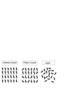
Figure 1: Illustrative pictures of the three phases as the temperature increases, low-temperature (ordered) solid, intermediate plastic crystal, and high-temperature (disordered) liquid phase. In the plastic state the centers of mass of the molecules form a regular crystalline lattice but the molecules are disordered with respect to the orientational degrees of freedom.

The so-called plastic crystals plastic1 ; brandreview ; folmer ; michel85 ; michel87 ; galam87 ; galam89 ; salinas1 ; salinas2 appear as states of some compounds considered to be simpler than those of canonical glasses, but still presenting rather nontrivial relaxation and equilibrium properties. Such a plastic phase corresponds to an intermediate stable state, between a high-temperature (disordered) liquid phase, and a low-temperature (ordered) solid phase and both transitions, namely, liquid-plastic and plastic-solid, are first order. In this intermediate phase, the rotational disorder coexists with a translationally ordered state, characterized by the centers of mass of the molecules forming a regular crystalline lattice with the molecules presenting disorder in their orientational degrees of freedom, as shown in Fig. 1. Many materials undergo a liquid-plastic phase transition, where the lower-temperature phase presents such a partial orientational order, like the plastic-crystal of Fig. 1. The property of translational invariance makes the plastic crystals much simpler to be studied from both analytical and numerical methods, becoming very useful towards a proper understanding of the glass transition plastic1 ; brandreview ; folmer . In some plastic-crystal models one introduces a coupling between two Ising models, associating each of these systems respectively, to the translational and rotational degrees of freedom galam87 ; galam89 ; salinas1 ; salinas2 , as a proposal for explaining satisfactorily thermodynamic properties of the plastic phase.

Accordingly, spin variables $\{t_{i}\}$ and $\{r_{i}\}$ are introduced in such a way to mimic translational and rotational degrees of freedom of each molecule $i$, respectively. The following Hamiltonian is considered galam87 ; galam89 ; salinas1 ; salinas2 ,

$${\cal H}=-J_{t}\sum_{\langle ij\rangle}t_{i}t_{j}-J_{r}\sum_{\langle ij\rangle}r_{i}r_{j}-\sum_{i}(\alpha t_{i}+h_{i})r_{i}~{},$$ (1)

where $\sum_{\langle ij\rangle}$ represents a sum over distinct pairs of nearest-neighbor spins. In the first summation, the Ising variables $t_{i}=\pm 1$ may characterize two lattices A and B (or occupied and vacant sites). One notices that the rotational variables $r_{i}$ could be, in principle, continuous variables, although the fact that the minimization of the coupling contribution $\alpha t_{i}r_{i}$ is achieved for $t_{i}r_{i}=1$ ($\alpha>0$), or for $t_{i}r_{i}=-1$ ($\alpha<0$), suggests the simpler choice of binary variables ($r_{i}=\pm 1$) to be appropriate, based on the energy minimization requirement.

In the present model the variables $t_{i}$ and $r_{i}$ represent very different characteristics of a molecule. Particularly, the rotational variables $r_{i}$ are expected to change more freely than the translational ones; for this reason, one introduces a random field acting only on the rotational degrees of freedom. In fact, the whole contribution $\sum_{i}(\alpha t_{i}+h_{i})r_{i}$ is known to play a fundamental role for the plastic phase of ionic plastic crystals, like the alkalicyanides KCN, NaCN and RbCN. In spite of its simplicity, the above Hamiltonian is able to capture the most relevant features of the plastic-crystal phase, as well as the associated phase transitions, namely, liquid-plastic and plastic-solid ones michel85 ; michel87 ; galam87 ; galam89 ; salinas1 ; salinas2 ; vives .

A system described by a Hamiltonian slightly different from the one of Eq. (1), in which the whole contribution $\sum_{i}(\alpha t_{i}+h_{i})r_{i}$ was replaced by $\sum_{i}\alpha_{i}t_{i}r_{i}$, i.e., with no random field acting on variable $r_{i}$ separately, was considered in Ref. salinas2 . In such a work one finds a detailed analysis of the phase diagrams and order-parameter behavior of the corresponding model. However, to our knowledge, previous investigations on the model defined by Eq. (1) have not considered thoroughly the effects of the random field $h_{i}$, with a particular attention to the phase diagrams for the case of a randomly distributed bimodal one, $h_{i}=\pm h_{0}$; this represents the main motivation of the present work. In the next section we define the model, determine its free-energy density, and describe the numerical procedure to be used. In Section III we exhibit typical phase diagrams and analyze the behavior of the corresponding order parameters, for both zero and finite temperatures; the ability of the model to exhibit a rich variety of phase diagrams, characterized by multicritical behavior, is shown. Finally, in Section IV we present our main conclusions.

II The Model and Free-Energy Density

Based on the discussion of the previous section, herein we consider a system composed by two interacting Ising models, described by the Hamiltonian

$${\cal H}(\{h_{i}\})=-J_{\sigma}\sum_{(ij)}\sigma_{i}\sigma_{j}-J_{\tau}\sum_{(ij)}\tau_{i}\tau_{j}+D\sum_{i=1}^{N}\tau_{i}\sigma_{i}-\sum_{i=1}^{N}h_{i}\tau_{i}~{},$$ (2)

where $\sum_{(ij)}$ represent sums over all distinct pairs of spins, a limit for which the mean-field approximation becomes exact. Moreover, $\tau_{i}=\pm 1$ and $\sigma_{i}=\pm 1$ ($i=1,2,\cdots,N$) depict Ising variables, $D$ stands for a real parameter, whereas both $J_{\sigma}$ and $J_{\tau}$ are positive coupling constants, which will be restricted herein to the symmetric case, $J_{\sigma}=J_{\tau}=J>0$. Although this later condition may seem as a rather artificial simplification of the Hamiltonian in Eq. (1), the application of a random field $h_{i}$ acting separately on one set of variables, will produce the expected distinct physical behavior associated with $\{\tau_{i}\}$ and $\{\sigma_{i}\}$. The random fields $\{h_{i}\}$ will be considered as following a symmetric bimodal probability distribution function,

$$P(h_{i})=\frac{1}{2}\,\delta(h_{i}-h_{0})+\frac{1}{2}\,\delta(h_{i}+h_{0})~{}.$$ (3)

The infinite-range character of the interactions allows one to write the above Hamiltonian in the form

$${\cal H}(\{h_{i}\})=-\frac{J}{2N}{\left(\sum_{i=1}^{N}\sigma_{i}\right)}^{2}-\frac{J}{2N}{\left(\sum_{i=1}^{N}\tau_{i}\right)}^{2}+D\sum_{i=1}^{N}\tau_{i}\sigma_{i}-\sum_{i=1}^{N}h_{i}\tau_{i}~{},$$ (4)

from which one may calculate the partition function associated with a particular configuration of the fields $\{h_{i}\}$,

$$Z(\{h_{i}\})={\rm Tr}\exp\left[-\beta{\cal H}(\{h_{i}\})\right]~{},$$ (5)

where $\beta=1/(kT)$ and ${\rm Tr}\equiv{\rm Tr}_{\{\tau_{i},\sigma_{i}=\pm 1\}}$ indicates a sum over all spin configurations. One can now make use of the Hubbbard-Stratonovich transformation dotsenkobook ; nishimoribook to linearize the quadratic terms,

$$Z(\{h_{i}\})=\frac{1}{\pi}\int_{-\infty}^{\infty}dxdy\exp(-x^{2}-y^{2})\prod_{i=1}^{N}{\rm Tr}\exp[H_{i}(\tau,\sigma)]~{},$$ (6)

where $H_{i}(\tau,\sigma)$ depends on the random fields $\{h_{i}\}$, as well as on the spin variables, being given by

$$H_{i}(\tau,\sigma)=\sqrt{\frac{2\beta J}{N}}\ x\tau+\sqrt{\frac{2\beta J}{N}}\ y\sigma-\beta D\tau\sigma+\beta h_{i}\tau~{}.$$ (7)

Performing the trace over the spins and defining new variables, related to the respective order parameters,

$$m_{\tau}=\sqrt{\frac{2kT}{JN}}\ x~{};\qquad m_{\sigma}=\sqrt{\frac{2kT}{JN}}\ y~{},$$ (8)

one obtains

$$Z(\{h_{i}\})=\frac{\beta JN}{2\pi}\int_{-\infty}^{\infty}dm_{\tau}dm_{\sigma}\exp[Ng_{i}(m_{\tau},m_{\sigma})]~{},$$ (9)

where

$$g_{i}(m_{\tau},m_{\sigma}) = -\frac{1}{2}\beta Jm_{\tau}^{2}-\frac{1}{2}\beta Jm_{\sigma}^{2}+\log\left\{2e^{-\beta D}\cosh[\beta J(m_{\tau}+m_{\sigma}+h_{i}/J)]\right.$$ (10)

$$+ \left.2e^{\beta D}\cosh[\beta J(m_{\tau}-m_{\sigma}+h_{i}/J)]\right\}~{}.$$

Now, one takes the thermodynamic limit ($N\rightarrow\infty$), and uses the saddle-point method to obtain

$$Z=\displaystyle\frac{\beta JN}{2\pi}\int_{-\infty}^{\infty}dm_{\tau}dm_{\sigma}\exp[-N\beta f(m_{\tau},m_{\sigma})]~{},$$ (11)

where the free-energy density functional $f(m_{\tau},m_{\sigma})$ results from a quenched average of $g_{i}(m_{\tau},m_{\sigma})$ in Eq. (10), over the bimodal probability distribution of Eq. (3),

$$f(m_{\tau},m_{\sigma})=\displaystyle\frac{1}{2}Jm_{\tau}^{2}+\frac{1}{2}Jm_{\sigma}^{2}-\frac{1}{2\beta}\log Q(h_{0})-\frac{1}{2\beta}\log Q(-h_{0})~{},$$ (12)

with

$$Q(h_{0})=2e^{-\beta D}\cosh[\beta J(m_{\tau}+m_{\sigma}+h_{0}/J)]+2e^{\beta D}\cosh[\beta J(m_{\tau}-m_{\sigma}+h_{0}/J)]~{}.$$ (13)

The extremization of the free-energy density above with respect to the parameters $m_{\tau}$ and $m_{\sigma}$ yields the following equations of state,

$$m_{\tau} = \frac{1}{2}\frac{R_{+}(h_{0})}{Q(h_{0})}+\frac{1}{2}\frac{R_{+}(-h_{0})}{Q(-h_{0})}~{},$$ (14)

$$m_{\sigma} = \frac{1}{2}\frac{R_{-}(h_{0})}{Q(h_{0})}+\frac{1}{2}\frac{R_{-}(-h_{0})}{Q(-h_{0})}~{},$$ (15)

where

$$R_{\pm}(h_{0})=e^{-\beta D}\sinh[\beta J(m_{\tau}+m_{\sigma}+h_{0}/J)]\pm e^{\beta D}\sinh[\beta J(m_{\tau}-m_{\sigma}+h_{0}/J)]~{}.$$ (16)

In the following section we present numerical results for the order parameters and phase diagrams of the model, at both zero and finite temperatures. All phase diagrams are represented by rescaling conveniently the energy parameters of the system, namely, $kT/J$, $h_{0}/J$ and $D/J$. Therefore, for given values of these dimensionless parameters, the equations of state [Eqs.(14) and (15)] are solved numerically for $m_{\tau}$ and $m_{\sigma}$. In order to avoid metastable states, all solutions obtained for $m_{\tau}\in[-1,1]$ and $m_{\sigma}\in[-1,1]$ are substituted in Eq. (12), to check for the minimization of the free-energy density. The continuous (second order) critical frontiers are found by the set of input values for which the order parameters fall continuously down to zero, whereas the first-order frontiers were found through Maxwell constructions.

Both ordered ($m_{\tau}\neq 0$ and $m_{\sigma}\neq 0$) and partially-ordered ($m_{\tau}=0$ and $m_{\sigma}\neq 0$) phases have appeared in our analysis, and will be labeled accordingly. The usual paramagnetic phase (P), given by $m_{\tau}=m_{\sigma}=0$, always occurs for sufficiently high temperatures. A wide variety of critical points appeared in our analysis (herein we follow the classification due to Griffiths griffiths ): (i) a tricritical point signals the encounter of a continuous frontier with a first-order line with no change of slope; (ii) an ordered critical point corresponds to an isolated critical point inside the ordered region, terminating a first-order line that separates two distinct ordered phases; (ii) a triple point, where three distinct phases coexist, signaling the encounter of three first-order critical frontiers. In the phase diagrams we shall use distinct symbols and representations for the critical points and frontiers, as described below.

• Continuous (second order) critical frontier: continuous line;

• First-order critical frontier: dotted line;

• Tricritical point: located by a black circle;

• Ordered critical point: located by a black asterisk;

• Triple point: located by an empty triangle.

III Phase Diagrams and Behavior of Order Parameters

III.1 Zero-Temperature Analisis

At $T=0$, one has to analyze the different spin orderings that minimize the Hamiltonian of Eq. (4). Due to the coupling between the two sets of spins, the minimum-energy configurations will correspond to $\{\tau_{i}\}$ and $\{\sigma_{i}\}$ antiparallel ($D>0$), or parallel ($D<0$). Therefore, in the absence of random fields ($h_{0}=0$) one should have $m_{\tau}=-m_{\sigma}$ ($D>0$), and $m_{\tau}=m_{\sigma}$ ($D<0$), where $m_{\sigma}=\pm 1$. However, when random fields act on the $\{\tau_{i}\}$ spins, there will be a competition between these fields and the coupling parameter $D$, leading to several phases, as represented in Fig. 2, in the plane $h_{0}/J$ versus $D/J$. One finds three ordered phases for sufficiently low values of $h_{0}/J$ and $|D|/J$, in addition to P phases for $(|D|/J)>0.5$ and $(h_{0}/J)>1$. All frontiers shown in Fig. 2 are first-order critical lines.

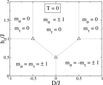
Figure 2: Phase diagram of the model defined by Hamiltonian of Eq. (4), at zero temperature. All critical frontiers represent first-order phase transitions; the empty triangles denote triple points.

When $(h_{0}/J)\leq 1/2$ one finds ordered phases for all values of $D/J$, with a vertical straight line at $D=0$ separating the symmetric state ($D<0$), where $m_{\tau}=m_{\sigma}$, from the antisymmetric one ($D>0$), characterized by $m_{\tau}=-m_{\sigma}$. Two critical frontiers (symmetric under a reflection operation) emerge from the triple point at $(D/J)=0.0$ and $(h_{0}/J)=0.5$, given, respectively, by $(h_{0}/J)=0.5+(D/J)$ for $D>0$, and $(h_{0}/J)=0.5-(D/J)$ for $D<0$. These critical frontiers terminate at $(h_{0}/J)=1.0$ and separate the low random-field-valued ordered phases from a partially-ordered phase, given by $m_{\tau}=0$ and $m_{\sigma}=\pm 1$. As shown in Fig. 2, three triple points appear, each of them signaling the encounter of three first-order lines, characterized by a coexistence of three phases, defined by distinct values of the magnetizations $m_{\tau}$ and $m_{\sigma}$, as described below.

• $[(D/J)=-0.5$ and $(h_{0}/J)=1.0]$ : $(m_{\tau},m_{\sigma})=\{(0,0);(0,\pm 1);(\pm 1,\pm 1)\}$.

• $[(D/J)=0.5$ and $(h_{0}/J)=1.0]$ : $(m_{\tau},m_{\sigma})=\{(0,0);(0,\pm 1);(\pm 1,\mp 1)\}$.

• $[(D/J)=0.0$ and $(h_{0}/J)=0.5]$ : $(m_{\tau},m_{\sigma})=\{(\pm 1,\pm 1);(\pm 1,\mp 1);(0,\pm 1)\}$.

Such a rich critical behavior shown for $T=0$ suggests that interesting phase diagrams should occur when the temperature is taken into account. From now on, we investigate the model defined by the Hamiltonian of Eq. (4) for finite temperatures.

III.2 Finite-Temperature Analysis

As shown above, the zero-temperature phase diagram presents a reflection symmetry with respect to $D=0$ (cf. Fig. 2). The only difference between the two sides of this phase diagram concerns the magnetization solutions characterizing the ordered phases for low random-field values, where one has $m_{\tau}=-m_{\sigma}$ ($D>0$), or $m_{\tau}=m_{\sigma}$ ($D<0$). These results come as a consequence of the symmetry of the Hamiltonian of Eq. (4), which remains unchanged under the operations, $D\rightarrow-D$, $\sigma_{i}\rightarrow-\sigma_{i}$ $(\forall i)$, or $D\rightarrow-D$, $\tau_{i}\rightarrow-\tau_{i}$, $h_{i}\rightarrow-h_{i}$ $(\forall i)$. Hence, the finite-temperature phase diagrams should present similar symmetries with respect to a change $D\rightarrow-D$. From now on, for the sake of simplicity, we will restrict ourselves to the case $(D/J)\geq 0$, for which the zero-temperature and low-random-field magnetizations present opposite signals, as shown in Fig. 2, i.e., $m_{\tau}=-m_{\sigma}$ .

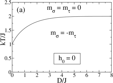
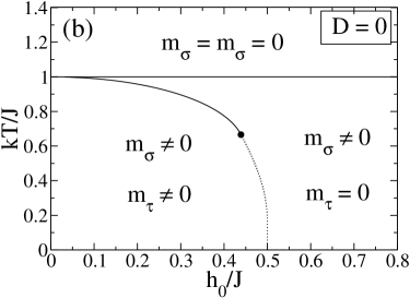
Figure 3: Phase diagrams of the model defined by the Hamiltonian of Eq. (4) in two particular cases: (a) The plane of dimensionless variables $kT/J$ versus $D/J$, in the absence of random fields $(h_{0}=0)$; (b) The plane of dimensionless variables $kT/J$ versus $h_{0}/J$, for $D=0$. The full lines represent continuous phase transitions, whereas the dotted line stands for a first-order critical frontier. For sufficiently high temperatures one finds a paramagnetic phase (P), whereas the magnetizations $m_{\tau}$ and $m_{\sigma}$ become nonzero by lowering the temperature. In case (b), two low-temperature phases appear, namely, the ordered (lower values of $h_{0}$) and the partially-ordered (higher values of $h_{0}$). These two phases are separated by a continuous critical frontier (higher temperatures), which turns into a first-order critical line (lower temperatures) at a tricritical point (black circle). The type of phase diagram exhibited in (b) will be called herein of topology I.

In Fig. 3 we exhibit phase diagrams of the model in two particular cases, namely, in the absence of fields $(h_{0}=0)$ [Fig. 3(a)] and for zero coupling $(D=0)$ [Fig. 3(b)]. These figures provide useful reference data in the numerical procedure to be employed for constructing phase diagrams in more general situations, e.g., in the plane $kT/J$ versus $h_{0}/J$, for several values of $(D/J)>0$.

In Fig. 3(a) we present the phase diagram of the model in the plane of dimensionless variables $kT/J$ versus $D/J$, in the absence of random fields ($h_{0}=0$), where one sees the point $D=0$ that corresponds to two noninteracting Ising models, leading to the well-known mean-field critical temperature of the Ising model [$(kT_{c}/J)=1$]. Also in Fig. 3(a), the ordered solution $m_{\tau}=-m_{\sigma}$ minimizes the free energy at low temperatures for any $D>0$; a second-order frontier separates this ordered phase from the paramagnetic one that appears for sufficiently high temperatures. For high values of $D/J$ one sees that this critical frontier approaches asymptotically $(kT/J)=2$. Since the application of a random field results in a decrease of the critical temperature, when compared with the one of the case $h_{0}=0$ aharony ; mattis ; kaufman , the result of Fig. 3(a) shows that no ordered phase should occur for $h_{0}>0$ and $(kT/J)>2$.

The phase diagram for $D=0$ is shown in the plane of dimensionless variables $kT/J$ versus $h_{0}/J$ in Fig. 3(b). The P phase occurs for $(kT/J)>1$, whereas for $(kT/J)<1$ two phases appear, namely, the ordered one (characterized by $m_{\sigma}\neq 0$ and $m_{\tau}\neq 0$, with $|m_{\sigma}|\geq|m_{\tau}|$), as well as the partially-ordered phase ($m_{\sigma}\neq 0$ and $m_{\tau}=0$). Since the two Ising models are uncorrelated for $D=0$ and the random fields act only on the $\{\tau_{i}\}$ variables, one finds that the critical behavior associated with variables $\{\sigma_{i}\}$ and $\{\tau_{i}\}$ occur independently: (i) The variables $\{\sigma_{i}\}$ order at $(kT/J)=1$, for all values of $h_{0}$; (ii) The critical frontier shown in Fig. 3(b), separating the two low-temperature phases, is characteristic of an Ising ferromagnet in the presence of a bimodal random field aharony . The black circle denotes a tricritical point, where the higher-temperature continuous frontier meets the lower-temperature first-order critical line. The type of phase diagram exhibited in Fig. 3(b) will be referred herein as topology I.

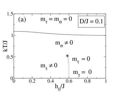
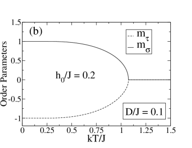
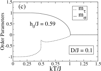
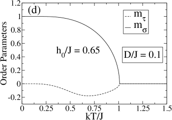
Figure 4: Phase diagram and order parameters in the case $(D/J)=0.1$. (a) Phase diagram in the plane of dimensionless variables $kT/J$ versus $h_{0}/J$. At low temperatures, a first-order critical frontier that terminates in an ordered critical point (black asterisk) separates the ordered phase (lower values of $h_{0}/J$) from the partially-ordered phase (higher values of $h_{0}/J$); this type of phase diagram will be referred herein as topology II. The order parameters $m_{\tau}$ and $m_{\sigma}$ are represented versus the dimensionless temperature $kT/J$ for typical values of $h_{0}/J$: (b) As one goes through the ordered phase (low temperatures) to the P phase; (c) As one goes through the first-order critical frontier, which separates the two ordered phases, up to the P phase; (d) As one goes through the partially-ordered phase (slightly to the right of the first-order critical frontier) up to the P phase. Equivalent solutions exist by inverting the signs of $m_{\tau}$ and $m_{\sigma}$.

The effects of a small interaction [$(D/J)=0.1$] between the variables $\{\sigma_{i}\}$ and $\{\tau_{i}\}$ are presented in Fig. 4, where one sees that the topology I [Fig. 3(b)] goes through substantial changes, as shown in Fig. 4(a) (to be called herein as topology II). As expected from the behavior presented in Fig. 3(a), one notices that the border of the P phase (a continuous frontier) is shifted to higher temperatures. However, the most significant difference between topologies I and II consists in the low-temperature frontier separating the ordered and partially-ordered phases. Particularly, the continuous frontier, as well as the tricritical point shown in Fig. 3(b), give place to an ordered critical point griffiths , at which the low-temperature first-order critical frontier terminates. Such a topology has been found also in some random magnetic systems, like the Ising and Blume-Capel models, subject to random fields and/or dilution kaufman ; salmon1 ; salmon2 ; benyoussef ; carneiro ; kaufmankanner . In the present model, we verified that topology II holds for any $0<(D/J)<1/2$, with the first-order frontier starting at zero temperature and $(h_{0}/J)=(D/J)+1/2$, which in Fig. 4(a) corresponds to $(h_{0}/J)=0.6$. Such a first-order line essentially affects the parameter $m_{\tau}$, as will be discussed next.

In Figs. 4(b)–(d) the order parameters $m_{\tau}$ and $m_{\sigma}$ are exhibited versus $kT/J$ for conveniently chosen values of $h_{0}/J$, corresponding to distinct physical situations of the phase diagram for $(D/J)=0.1$. A curious behavior is presented by the magnetization $m_{\tau}$ by varying $h_{0}/J$, and more particularly, around the first-order critical line. For $(h_{0}/J)=0.59$ [Fig. 4(c)], one starts at low temperatures essentially to the left of the critical frontier and by increasing $kT/J$ one crosses this critical frontier at $(kT/J)=0.499$, very close to the ordered critical point. At this crossing point, $|m_{\tau}|$ presents an abrupt decrease, i.e., a discontinuity, corresponding to a change to the partially-ordered phase; on the other hand, the magnetization $m_{\sigma}$ remains unaffected when going through this critical frontier. For higher temperatures, $|m_{\tau}|$ becomes very small, but still finite, turning up zero only at the P boundary; in fact, the whole region around the ordered critical point is characterized by a finite small value of $|m_{\tau}|$. Another unusual effect is presented in Fig. 4(d), for which $(h_{0}/J)=0.65$, i.e., slightly to the right of the first-order critical frontier: the order parameter $m_{\tau}$ is zero for low temperatures, but becomes nonzero by increasing the temperature, as one becomes closer to the critical ordered point. This rather curious phenomenon is directly related to the correlation between the variables $\{\sigma_{i}\}$ and $\{\tau_{i}\}$: since for $(kT/J)\approx 0.5$ the magnetization $m_{\sigma}$ is still very close to its maximum value, a small value for $|m_{\tau}|$ is induced, so that both order parameters go to zero together only at the P frontier.

Behind the results presented in Figs. 4(a)–(d) one finds a very interesting feature, namely, the possibility of going continuously from the ordered phase to the partially-ordered phase by circumventing the ordered critical point. This is analogous to what happens in many substances, e.g., water, where one goes continuously (with no latent heat) from the liquid to the gas phase by circumventing a critical end point huang ; reichl .

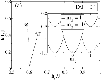
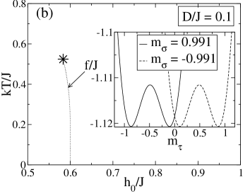
Figure 5: The first-order critical line in Fig. 4(a), corresponding to $(D/J)=0.1$, is amplified, and the dimensionless free-energy density $f/J$ of Eq. (12) (shown in the insets) is analyzed at two distinct points along this frontier: (a) A low-temperature point located at $[(h_{0}/J)=0.599,(kT/J)=0.010]$, showing the coexistence of the ordered ($|m_{\tau}|=1$) and partially-ordered ($m_{\tau}=0$) solutions; (b) A higher-temperature point located at $[(h_{0}/J)=0.594,(kT/J)=0.387]$, showing the coexistence of solutions with $|m_{\tau}|>0$, namely, $|m_{\tau}|=0.868$ and $|m_{\tau}|=0.1$. In both cases (a) and (b) the free energy presents four minima, associated with distinct pairs of solutions $(m_{\tau},m_{\sigma})$: the full lines show the two minima with positive $m_{\sigma}$, whereas the dashed lines correspond to the two minima with negative $m_{\sigma}$.

In Fig. 5 the free-energy density of Eq. (12) is analyzed at two different points along the first-order critical frontier of Fig. 4(a), namely, a low-temperature one [Fig. 5(a)], and a point at a higher temperature [Fig. 5(b)]. In both cases the free energy presents four minima associated with distinct pairs of solutions $(m_{\tau},m_{\sigma})$. The point at $(kT/J)=0.010$ presents $(m_{\tau},m_{\sigma})=\{(-1,1);(0,1);(0,-1);(1,-1)\}$, whereas the point at $(kT/J)=0.387$ presents $(m_{\tau},m_{\sigma})=\{(-0.868,0.991);(-0.100,0.991);(0.100,-0.991);(0.868,-0.991)\}$. The lower-temperature point represents a coexistence of the two phases shown in the case $D=0$ [cf. Fig. 3(b)], namely, the ordered ($|m_{\tau}|=1$) and partially-ordered ($m_{\tau}=0$) phases. However, the higher-temperature point typifies the phenomenon discussed in Fig. 4, where distinct solutions with $|m_{\tau}|>0$ coexist, leading to a jump in this order parameter as one crosses the critical frontier, like illustrated in Fig. 4(c) for the point $[(h_{0}/J)=0.59,(kT/J)=0.499]$. Although the magnetization $m_{\tau}$ presents a very curious behavior in topology II [cf., e.g., Figs. 4(b)–(d)], $m_{\sigma}$ remains essentially unchanged by the presence of the first-order critical frontier of Fig. 4(a), as shown also in Fig. 5.

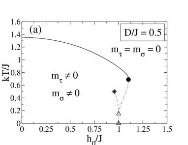
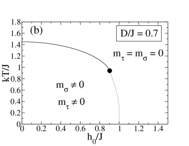
Figure 6: Phase diagrams in the plane of dimensionless variables $kT/J$ versus $h_{0}/J$ for two different values of $D/J$: (a) $(D/J)=0.5$, to be referred as topology III; (b) $(D/J)=0.7$, to be referred as topology IV.

In Fig. 6 we present two other possible phase diagrams, namely, the cases $(D/J)=0.5$ [Fig. 6(a), called herein topology III] and $(D/J)=0.7$ [Fig. 6(b), called herein topology IV]. Whereas topology III represents a special situation that applies only for $(D/J)=0.5$, exhibiting the richest critical behavior of the present model, topology IV holds for any $(D/J)>0.5$. In Fig. 6(a) one observes the appearance of several multicritical points, denoted by the black circle (tricritical point), black asterisk (ordered critical point), and empty triangles (triple points): (i) The tricritical point, which signals the encounter of the higher-temperature continuous phase transition with the lower-temperature first-order phase transition, found in the $D=0$ phase diagram [cf. Fig. 3(b)], have curiously disappeared for $0<(D/J)<0.5$, and emerged again for $(D/J)=0.5$; (ii) The ordered critical point exists for any $0<(D/J)\leq 0.5$ [as shown in Fig. 4(a)]; (iii) Two triple points, one at a finite temperature, whereas the other one occurs at zero temperature. It should be mentioned that such a zero-temperature triple point corresponds precisely to the one of Fig. 2, at $(D/J)=0.5$ and $(h_{0}/J)=1.0$. The value $(D/J)=0.5$ is very special and will be considered as a threshold for both multicritical behavior and correlations between the two systems. We have observed that for $(D/J)\gtrsim 0.5$, the critical points shown in Fig. 6(a) disappear, except for the tricritical point that survives for $(D/J)>0.5$ [as shown in Fig. 6(b)]. Changes similar to those occurring herein between topologies II and III, as well as topologies III and IV, were found also in some magnetic systems, like the Ising and Blume-Capel models, subject to random fields and/or dilution kaufman ; salmon1 ; salmon2 ; benyoussef ; carneiro ; kaufmankanner . Particularly, the splitting of the low-temperature first-order critical frontier into two higher-temperature first-order lines that terminate in the ordered and tricritical points, respectively [as exhibited in Fig. 6(a)], is consistent with results found in the Blume-Capel model under a bimodal random magnetic, by varying the intensity of the crystal field kaufmankanner .

Another important feature of topology III concerns the lack of any type of magnetic order at finite temperatures for $(h_{0}/J)>1.1$, in contrast to the phase diagrams for $0\leq(D/J)<0.5$, for which there is $m_{\sigma}\neq 0$ for all $h_{0}/J$ [see, e.g., Figs. 3(b) and 4(a)]. This effect shows that $(D/J)=0.5$ represents a threshold value for the coupling between the variables $\{\sigma_{i}\}$ and $\{\tau_{i}\}$, so that for $(D/J)\geq 0.5$ the correlations among these variables become significant. As a consequence of these correlations, the fact of no magnetic order on the $\tau$-system ($m_{\tau}=0$) drives the the magnetization of the $\sigma$-system to zero as well, for $(h_{0}/J)>1.1$. It is important to notice that the $T=0$ phase diagram of Fig. 2 presents a first-order critical line for $(D/J)=0.5$ and $(h_{0}/J)>1.0$, at which $m_{\tau}=0$, whereas in the $\sigma$-system both $m_{\sigma}=0$ and $|m_{\sigma}|=1$ minimize the Hamiltonian. By analyzing numerically the free-energy density of Eq. (12) at low temperatures and $(h_{0}/J)>1.0$, we have verified that for any infinitesimal value of $kT/J$ destroys such a coexistence of solutions, leading to a minimum free energy at $m_{\tau}=m_{\sigma}=0\ (\forall\,T>0)$. Consequently, one finds that the low-temperature region in the interval $1.0\leq(h_{0}/J)\leq 1.1$ becomes part of the P phase. Hence, the phase diagram in Fig. 6(a) presents a reentrance phenomena for $1.0\leq(h_{0}/J)\leq 1.1$. In this region, by lowering the temperature gradually, one goes from a P phase to the ordered phase ($m_{\tau}\neq 0$ ; $m_{\sigma}\neq 0$), and then back to the P phase. This effect appears frequently in both theoretical and experimental investigations of disordered magnets dotsenkobook ; nishimoribook .

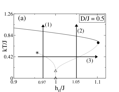
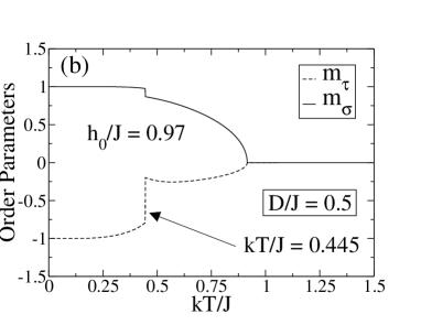
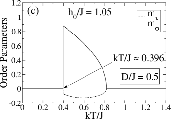
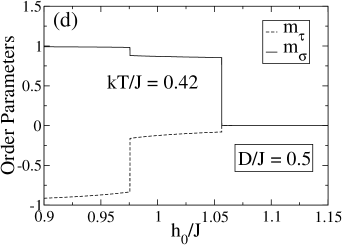
Figure 7: (a) The region of multicritical points of the phase diagram for $(D/J)=0.5$ [Fig. 6(a)] is amplified and three thermodynamic paths are chosen for analyzing the magnetizations $m_{\tau}$ and $m_{\sigma}$. (b) Order parameters along thermodynamic path (1): $(h_{0}/J)=0.97$ and increasing temperatures. (c) Order parameters along thermodynamic path (2): $(h_{0}/J)=1.05$ and increasing temperatures. (d) Order parameters along thermodynamic path (3): $(kT/J)=0.42$ and varying the field strength in the interval $0.9\leq(h_{0}/J)\leq 1.15$. Equivalent solutions exist by inverting the signs of $m_{\tau}$ and $m_{\sigma}$.

In Fig. 7 we analyze the behavior of the $m_{\tau}$ and $m_{\sigma}$ for topology III, in the region of multicritical points of the phase diagram for $(D/J)=0.5$, along three typical thermodynamic paths, as shown in Fig. 7(a). In Fig. 7(b) we exhibit the behavior of $m_{\tau}$ and $m_{\sigma}$ along path (1), where one sees that both parameters go through a jump by crossing the first-order critical line [$(kT/J)=0.445$], expressing a coexistence of different types of solutions for $m_{\tau}$ and $m_{\sigma}$ at this point. One notices a larger jump in $m_{\tau}$, so that to the right of the ordered critical point one finds a behavior similar to the one verified in topology II, where $|m_{\tau}|$ becomes very small, whereas $m_{\sigma}$ still presents significant values. Then, by further increasing the temperature, these parameters tend smoothly to zero at the continuous critical frontier separating the ordered and P phases. In Fig. 7(c) we show the magnetizations $m_{\tau}$ and $m_{\sigma}$ along path (2), within the region of the phase diagram where the reentrance phenomenon occurs; along this path, one increases the temperature, going from the P phase to the ordered phase and then to the P phase again. Both parameters are zero for low enough temperatures, jumping to nonzero values at $(kT/J)=0.396$, as one crosses the first-order critical line. After such jumps, by increasing the temperature, these parameters tend smoothly to zero at the border of the P phase. The behavior shown in Fig. 7(c) confirm the reentrance effect, discussed previously. Finally, in Fig. 7(d) we exhibit the order parameters along thermodynamic path (3), for which the temperature is fixed at $(kT/J)=0.42$, with the field varying in the range $0.9\leq(h_{0}/J)\leq 1.15$. One sees that both magnetizations $m_{\tau}$ and $m_{\sigma}$ display jumps as one crosses each of the two first-order lines, evidencing a coexistence of different ordered states at the lower-temperature jump, as well as a coexistence of the ordered and P states at the higher-temperature jump.

The behavior presented by the order parameters in Figs. 7(b)–(d) shows clearly the fact that $(D/J)=0.5$ represents a threshold value for the coupling between the variables $\{\sigma_{i}\}$ and $\{\tau_{i}\}$. In all these cases, one sees that jumps in the magnetization $m_{\sigma}$ are correlated with corresponding jumps in $m_{\tau}$. These results should be contrasted with those for the cases $(D/J)<0.5$, as illustrated in Fig. 4(c), where a discontinuity in $m_{\tau}$ does not affect the smooth behavior presented by $m_{\sigma}$.

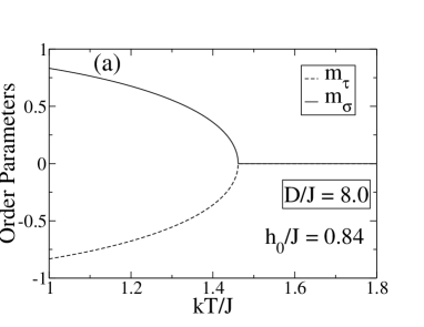
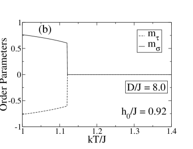
Figure 8: The order parameters $m_{\tau}$ and $m_{\sigma}$ are represented versus the dimensionless temperature $kT/J$ for $(D/J)=8.0$ and two typical values of $h_{0}/J$: (a) Slightly to the left of the tricritical point; (b) Slightly to the right of the tricritical point. The associated phase diagram corresponds to topology IV [cf. Fig. 6(b)]. Equivalent solutions exist by inverting the signs of $m_{\tau}$ and $m_{\sigma}$.

The phase diagram shown in Fig. 6(b), which corresponds to topology IV, is valid for any for any $(D/J)>0.5$. Particularly, the critical point where the low-temperature first-order critical frontier touches the zero-temperature axis is kept at $(h_{0}/J)=1$, for all $(D/J)>0.5$, in agreement with Fig. 2. We have verified only quantitative changes in such a phase diagram by increasing the coupling between the variables $\{\sigma_{i}\}$ and $\{\tau_{i}\}$. Essentially, the whole continuous critical frontier moves towards higher temperatures, leading to an increase in the values of the critical temperature for $(h_{0}/J)=0$, as well as in the temperature associated with the tricritical point, whereas the abscissa of this point remains typically unchanged. Moreover, in what concerns the order parameters, the difference between $|m_{\tau}|$ and $m_{\sigma}$ decreases, in such a way that for $(D/J)\rightarrow\infty$, one obtains $m_{\tau}=-m_{\sigma}$. This later effect is illustrated in Fig. 8, where we represent the order parameters $m_{\tau}$ and $m_{\sigma}$ versus temperature, for a sufficiently large value of $D/J$, namely, $(D/J)=8.0$, in two typical choices of $h_{0}/J$, close to the tricritical point. In Fig. 8(a) $m_{\tau}$ and $m_{\sigma}$ are analyzed slightly to the left of the tricritical point, exhibiting the usual continuous behavior, whereas in Fig. 8(b) they are considered slightly to the right of the tricritical point, presenting jumps as one crosses the first-order critical frontier. However, the most important conclusion from Fig. 8 concerns the fact that in both cases one has essentially $m_{\tau}=-m_{\sigma}$, showing that the random field applied solely to the $\tau$-system influences the $\sigma$-system in a similar way, due to the high value of $D/J$ considered. We have verified that for $(D/J)=8.0$ the two systems become so strongly correlated, such that $m_{\tau}=-m_{\sigma}$ holds along the whole phase diagram, within our numerical accuracy.

IV Conclusions

We have analyzed the effects of a coupling $D$ between two Ising models, defined in terms of variables $\{\tau_{i}\}$ and $\{\sigma_{i}\}$. The model was considered in the limit of infinite-range interactions, where all spins in each system interact by means of an exchange coupling $J>0$, typical of ferromagnetic interactions. Motivated by a qualitative description of systems like plastic crystals, the variables $\{\tau_{i}\}$ and $\{\sigma_{i}\}$ would represent rotational and translational degrees of freedom, respectively. Since the rotational degrees of freedom are expected to change more freely than the translational ones, a random field acting only on the variables $\{\tau_{i}\}$ was considered. For this purpose, a bimodal random field, $h_{i}=\pm h_{0}$, with equal probabilities, was defined on the $\tau$-system. The model was investigated through its free energy and its two order parameters, namely, $m_{\tau}$ and $m_{\sigma}$.

We have shown that such a system presents a very rich critical behavior, depending on the particular choices of $D/J$ and $h_{0}/J$. Particularly, at zero temperature, the phase diagram in the plane $h_{0}/J$ versus $D/J$ exhibits ordered, partially-ordered, and disordered phases. This phase diagram is symmetric around $(D/J)=0$, so that for sufficiently low values of $h_{0}/J$ one finds ordered phases characterized by $m_{\sigma}=m_{\tau}=\pm 1$ ($D<0$) and $m_{\sigma}=-m_{\tau}=\pm 1$ ($D>0$). We have verified that $|D/J|=1/2$ plays an important role in the present model, such that at zero temperature one has the disordered phase ($m_{\sigma}=m_{\tau}=0$) for $|D/J|>1/2$ and $(h_{0}/J)>1$. Moreover, the partially-ordered phase, where $m_{\sigma}=\pm 1$ and $m_{\tau}=0$, occurs for $(h_{0}/J)>1/2+|D/J|$ and $|D/J|<1/2$. In this phase diagram all phase transitions are of the first-order type, and three triple points were found. In the case of plastic crystals, the sequence of transitions from the disordered to the partially-ordered, and then to the ordered phases, would correspond to the sequence of transitions from the liquid to the plastic crystal, and then to ordered crystal phases.

Due to the symmetry around $D=0$, the finite-temperature phase diagrams were considered only for $D>0$, for which the ordered phase was identified by $m_{\sigma}>0$ and $m_{\tau}<0$, whereas the partially-ordered phase by $m_{\sigma}>0$ and $m_{\tau}=0$ (equivalent solutions also exist by inverting the signs of these order parameters). Several phase diagrams in the plane $kT/J$ versus $h_{0}/J$ were studied, by varying gradually $D/J$. We have found four qualitatively different types of phase diagrams, denominated as topologies I [$(D/J)=0$], II [$0<(D/J)<1/2$], III [$(D/J)=1/2$], and IV [$(D/J)>1/2$]. Such a classification reflects the fact that $(D/J)=1/2$ represents a threshold value for the coupling between the variables $\{\sigma_{i}\}$ and $\{\tau_{i}\}$, so that for $(D/J)\geq 1/2$ the correlations among these variables become significant, as verified through the behavior of the order parameters $m_{\tau}$ and $m_{\sigma}$. From all these cases, only topology IV typifies a well-known phase diagram, characterized by a tricritical point, where the higher-temperature continuous frontier meets the lower-temperature first-order critical line. This phase diagram is qualitatively similar to the one found for the Ising ferromagnet in the presence of a bimodal random field aharony , and it does not present the herein physically relevant partially-ordered phase. For $(D/J)\geq 1/2$, even though the random field is applied only in the $\tau$-system, the correlations lead the $\sigma$-system to follow a qualitatively similar behavior.

The phase diagrams referred as topologies I and II exhibit all three phases. In the later case we have found a first-order critical line terminating at an ordered critical point, leading to the potential physical realization of going continuously from the ordered phase to the partially-ordered phase by circumventing this critical point. In these two topologies, the sequence of transitions from the disordered to the partially-ordered, and then to the ordered phase, represents the physical situation that occurs in plastic crystals. For conveniently chosen thermodynamic paths, i.e., varying temperature and random field appropriately, one may go from the liquid phase ($m_{\sigma}=m_{\tau}=0$), to a plastic-crystal phase ($m_{\sigma}\neq 0$; $m_{\tau}=0$), where the rotational degrees of freedom are found in a disordered state, and then, to an ordered crystal phase ($m_{\sigma}\neq 0$; $m_{\tau}\neq 0$).

From the point of view of multicritical behavior, topology III [$(D/J)=1/2$] corresponds to the richest type of phase diagram, being characterized by several critical lines and multicritical points; one finds its most complex criticality around $(h_{0}/J)=1$, signaling a great competition among the different types of orderings. Although the partially-ordered phase does not appear in this particular case, one has also the possibility of circumventing the ordered critical point, such as to reach a region of the phase diagram along which $|m_{\tau}|$ becomes very small, resembling a partially-ordered phase.

Since the infinite-range interactions among variables of each Ising system correspond to a limit where mean-field approach becomes exact, an immediate question concerns whether some of the results obtained above represent an artifact of such limit. Certainly, such a relevant point is directly related with the existence of some of these features in the associated short-range three-dimensional magnetic models. For example, the tricritical point found in topologies III and IV is essentially the same that appears within the mean-field approach of the Ising model in the presence of a bimodal random field. This later model has been extensively investigated on a cubic lattice through different numerical approaches, where the existence of this tricritical point is still very controversial. On the other hand, a first-order critical frontier terminating at an ordered critical point, and the fact that one can go from one phase to another by circumventing this point, represents a typical physical situation that occurs in real substances. The potential for exhibiting such a relevant feature represents an important advantage of the present model.

Finally, we emphasize that the rich critical behavior presented in the phase diagrams corresponding to topologies II and III suggest the range $0<(D/J)\leq 1/2$ as appropriate for describing plastic crystals. The potential of exhibiting successive transitions from the ordered to the partially-ordered and then to the disordered phase should be useful for a better understanding of these systems. Furthermore, the characteristic of going continuously from the ordered phase to the partially-ordered phase by circumventing an ordered critical point represents a typical physical situation that occurs in many substances, and opens the possibility for the present model to describe a wider range of materials.

Acknowledgments

The partial financial supports from CNPq, FAPEAM-Projeto-Universal-Amazonas, and FAPERJ (Brazilian agencies) are acknowledged.

References

- (1) K. Huang, Statistical Mechanics, second edition (John Wiley and Sons, New York, 1987).
- (2) L. E. Reichl, A Modern Course in Statistical Physics, second edition (John Wiley and Sons, New York, 1998).
- (3) A. Aharony, Phys. Rev. B 18, 3318 (1978).
- (4) D. C. Mattis, Phys. Rev. Lett. 55, 3009 (1985).
- (5) M. Kaufman, P. E. Kluzinger and A. Khurana, Phys. Rev. B 34, 4766 (1986).
- (6) E. Nogueira Jr., F. D. Nobre, F. A. da Costa, and S. Coutinho, Phys. Rev. E 57, 5079 (1998); Erratum, Phys. Rev. E 60, 2429 (1999).
- (7) N. Crokidakis and F. D. Nobre, J. Phys. Condens. Matter 20, 145211 (2008).
- (8) N. Crokidakis and F. D. Nobre, Phys. Rev. E 77, 041124 (2008).
- (9) O. R. Salmon, N. Crokidakis and F. D. Nobre, J. Phys.: Condens. Matter 21, 056005 (2009).
- (10) C. V. Morais, S. G. Magalhães, and F. D. Nobre, J. Stat. Mech. P01013 (2012).
- (11) A. Fernandez del Río, E. Korutcheva and J. de la Rubia, Complexity, 17, 31 (2012).
- (12) J. N. Sherwood, Ed., The Plastically Crystalline State (John Wiley and Sons, New York, 1979).
- (13) R. Brand, P. Lunkenheimer, and A. Loidl, J. Chem. Phys. 116, 10386 (2002).
- (14) J. C. W. Folmer, R. L. Withers, T. R. Welberry and J. D. Martin, Phys. Rev. B 77, 144205 (2008).
- (15) K. H. Michel, and J. M. Rowe, Phys. Rev. B 32, 5818 (1985).
- (16) K. H. Michel, and J. Naudts, J. Chem. Phys. 67, 547 (1987).
- (17) S. Galam, Phys. Lett. A 122, 271 (1987).
- (18) S. Galam and M. Gabay, Europhys. Lett. 8, 167 (1989).
- (19) S. Galam, V. B. Henriques and S. R. Salinas, Phys. Rev. B 42, 6720 (1990).
- (20) S. Galam, S. R. Salinas and Y. Shapir, Phys. Rev. B 51, 2864 (1995).
- (21) E. Vives and A. Planes, Phys. Rev. B 43, 13335 (1991).
- (22) V. Dotsenko, Introduction to the Replica Theory of Disordered Statistical Systems, Cambridge University Press, Cambridge, 2001.
- (23) H. Nishimori, Statistical Physics of Spin Glasses and Information Processing, Oxford University Press, Oxford 2001.
- (24) R. B. Griffiths, Phys. Rev. B 12, 345 (1975).
- (25) O. R. Salmon and J. Rojas, J. Phys. A: Math. Theor. 43, 125003 (2010).
- (26) A. Benyoussef, T. Biaz, M. Saber and M. Touzani, J. Phys. C 20, 5349 (1987).
- (27) C. E. I. Carneiro, V. B. Henriques and S. R. Salinas, J. Phys. A: Math. Gen. 23, 3383 (1990).
- (28) M. Kaufman and M. Kanner, Phys. Rev. B 42, 2378 (1990).