X-Shooter spectroscopy of young stellar objects:
V – Slow winds in T Tauri stars

Disks around T Tauri stars are known to lose mass, as best shown by the profiles of forbidden emission lines of low ionization species. At least two separate kinematic components have been identified, one characterised by velocity shifts of tens to hundreds km/s (HVC) and one with much lower velocity of few km/s (LVC). The HVC are convincingly associated to the emission of jets, but the origin of the LVC is still unknown. In this paper we analyze the forbidden line spectrum of a sample of 44 mostly low mass young stars in Lupus and $\sigma$ Ori observed with the X-Shooter ESO spectrometer. We detect forbidden line emission of O i, O ii, S ii, N i, and N ii, and characterize the line profiles as LVC, blue-shifted HVC and red-shifted HVC. We focus our study on the LVC. We show that there is a good correlation between line luminosity and both L_star and the accretion luminosity (or the mass-accretion rate) over a large interval of values (L_star$\sim 10^{-2}-1$ L_⊙; L_acc$\sim 10^{-5}-10^{-1}$ L_⊙; $\dot{M}_{acc}$$\sim 10^{-11}-10^{-7}$ M_⊙/yr). The lines show the presence of a slow wind ($V_{peak}<20$ km/s), dense ($n_{H}>10^{8}$ cm^-3), warm (T$\sim 5000-10000$ K), mostly neutral. We estimate the mass of the emitting gas and provide a value for the maximum volume it occupies. Both quantities increase steeply with the stellar mass, from $\sim 10^{-12}$ M_⊙ and $\sim 0.01$ AU³ for M_star$\sim 0.1$ M_⊙, to $\sim 3\times 10^{-10}$ M_⊙ and $\sim 1$ AU³ for M_star$\sim 1$ M_⊙, respectively. These results provide quite stringent constraints to wind models in low mass young stars, that need to be explored further.

1 Introduction

Circumstellar disks of gas and dust surround young stars from their birth for a period of few million years; during this time planetary systems may form and evolve. The disk structure and its evolution affect the conditions for the formation of planets and their properties (Dutrey et al., 2014; Alexander et al., 2014). Disks are dynamical structures, with gas and dust accreting onto the central stars, but also being expelled from the systems. In particular, the way mass-loss occurs and evolves with time has important consequences on the disk survival and on its properties.

Mass-loss from magnetized accretion disks is expected, due to the combined effect of rotation and magnetic fields; it is probably a very complex phenomenon, with different components: a so-called disk wind, due to the relic magnetic field that threads the disk at all distances from the star, an X-wind, which is launched in the region close to the star where the stellar magnetic field provides the pressure required to overcome the stellar gravity, and, possibly, a stellar wind, where gas from the central star is expelled from the system (see, e.g. Ferreira, 2013, and references therein). Under the action of the magnetic field, the gas is collimated and accelerated to terminal velocities of few hundred km/s, forming the bright jets observed in several young objects (e.g. Frank et al., 2014). As magnetocentrifugal winds extract angular momentum from the disk, they can control accretion (e.g. Turner et al., 2014).

Disks can lose mass also when their upper layers are heated to temperatures such that the gas thermal energy exceeds its binding energy, and the gas escapes from the system (photoevaporation). This mechanism was firstly recognized to lead to dispersal of disks in the vicinity of a hot star (e.g., O’Dell & Wen, 1994). More recently, it has been realized that the combined effect of the high energy photons (UV, FUV, X) emitted by low-mass stars can heat the disk surface to sufficiently high temperatures to produce a centrifugally launched ouflow, driven by thermal pressure. Photoevaporation winds are possibly the cause of the quick disk dissipation, which ends their much longer phase of viscous evolution (see, e.g. Alexander et al., 2014, and references therein).

Observational evidence of mass-loss from young stars (T Tauri stars; TTS) with disks (Class II) is provided by the intensity and profiles of forbidden lines of atomic and low-ionization species, which present at least two different components (Hartigan et al., 1995). One is emitted by gas moving at high velocity (HVC), which is clearly identified with the jets that have been imaged and carefully studied in several objects. The other component is originated by a much slower moving gas (low-velocity component-LVC). The LVC is detected in most Class II objects, and its origin is still unknown. It could be emitted at the base of a magnetically driven disk wind, as suggested by Hartigan et al. (1995) for the O i lines, but it can also be a tracer of a photoevaporative disk wind, as shown by, e.g., Pascucci & Sterzik (2009) for the LVC of the Ne ii mid-IR emission lines. Lately, Rigliaco et al. (2013) have shown that the LVC O i lines could also have multiple components, with one component tracing gas in keplerian rotation, and another component tracing a photoevaporative wind. Acke et al. (2005) find that in Herbig Ae/Be stars, the [O i] 630.03nm emission could come from the disk surface layers. In this paper we will focus on the properties of the LVC components of the winds from low-mass T Tauri stars.

As for other disk and stellar diagnostics, to find meaningful trends and to make full use of the diagnostic potential of the LVC forbidden line emission, it is necessary to analyze simultaneously as many lines as possible and to have access to a large sample of objects, covering a wide range of stellar and accretion properties. The best sample available so far is still that of Hartigan et al. (1995), who observed 42 TTS in Taurus and detected forbidden line emission in about 30 of them. The number of stars with reliable measurements of the mass-accretion properties is, however, smaller, of the order of 12–15 objects (Gullbring et al., 1998; Rigliaco et al., 2013), mostly of relatively high mass and accretion rate. In this paper, we analyze a sample of 44 low-mass stars in two star-forming regions, Lupus and $\sigma$ Ori, of age  1–3 My. The two regions differ mostly due to the presence of a massive star ($\sigma$ Ori) in the $\sigma$ Ori region. The spectra have been obtained with X-Shooter@VLT (Vernet et al., 2011), which gives medium-resolution spectra simultaneously over the spectral range from 310 to 2500 nm. They have been collected as part of the Italian GTO (Alcalá et al., 2011) and have already been used to derive the stellar parameters and the accretion properties of the stars (Rigliaco et al., 2012; Alcalá et al., 2014). This is, therefore, the largest sample of TTS with well-known accretion properties studied so far with the aim of characterizing the mass-loss phenomenon and its origin.

In general, forbidden lines in the optical and near-IR are emitted by warm gas (temperature of few thousand degrees), where collisions with electrons or neutral hydrogen excite the upper levels of the transitions, and we will assume that this is the case throught this paper. However, an alternative, non-thermal mechanism has been proposed for the formation of the O i lines, namely that they have origin in a cooler disk region where OH is photodissociated by the stellar FUV photons (Acke et al., 2005; Gorti et al., 2011). We will come back to this point at the end of the paper.

The paper is organized as follows. §2 and 3 briefly summarize the observations and data reduction, and the sample properties, already discussed in (Alcalá et al., 2014; Rigliaco et al., 2012); §4 presents the forbidden line spectra; §5 the line profiles and the separation of the HVC and LVC. §6 is dedicated to the LVC. Discussion and summary follow in §7 and §8, respectively.

2 Observations

In this work we use the spectra published in Alcalá et al. (2014) and Rigliaco et al. (2012). The instrument setup, including the spectral resolution in each wavelength range and the corresponding signal-to-noise ratio, as well as the data reduction and calibration procedures and the derivation of extinction, spectral type and accretion luminosity are described in those papers. All the spectra used in this paper have been corrected for extinction. For most targets, the slit width was 1 arcsec, yielding a resolution of $\sim$60 km/s in the UVB arm and $\sim$35 km/s in the VIS arm.

In addition to the wavelength calibrations described in Alcalá et al. (2014) and Rigliaco et al. (2012) we have cross checked and adjusted the wavelength scale of the UVB and VIS arms by aligning the [O i] 557.79 line, which is covered by both arms. This line is detected in all objects for which we have detections of other lines in the UVB arm, with the exception of SO587 and SO646. We detected and applied an offset to the UVB wavelength calibration only in 8 cases out of 31 objects, in those cases the offset between the two scales was less than 24 km/s. We assumed zero offset for SO587 and SO646. The emission line velocities reported in this paper are all relative to the photospheric rest velocity as measured by the Li i line at 670.78 nm.

All the measurements of the [O i] 557.79 line used for the scientific analysis in this paper come from the UVB arm. While the spectral resolution in this arm is lower than in the VIS, the signal to noise at the wavelength of the [O i] 557.79 line is better.

3 The sample

The sample studied in this paper comprises 36 low-mass Class II (i.e., with evidence of disk from the infrared) stars in Lupus (2 of these are brown dwarfs) and 8 in $\sigma$ Ori. The spectra are publicly available in Vizier (J/A+A/561/A2 and J/A+A/548/A56). The Lupus sample contains about 50% of the total Class II population and is well representative of the properties of the region, while the number of objects in $\sigma$ Ori is small and the targets were selected among low-mass Class II objects in different locations with respect to the bright star $\sigma$ Ori. The objects are listed in Table 3, which gives the stellar parameters and the accretion luminosity and mass accretion rates from Alcalá et al. (2014) for objects in Lupus and Rigliaco et al. (2012) for the $\sigma$ Ori stars. As detailed in those papers, the X-Shooter spectrum of each object is described as the sum of the photospheric emission, taken to be that of non-accreting diskless young objects (Class III; see Manara et al. (2013)), and of a slab of hydrogen that represents the emission of the accretion shock. The spectral type, extinction and slab luminosity (i.e., the accretion luminosity) are therefore self-consistently determined. In the following, we will refer to stars in Table 3 as the Lupus and $\sigma$ Ori GTO (GTO for simplicity) sample.

The distribution of the stars in mass and accretion luminosity is shown in Figure 1. About 70% of the objects have masses $<0.3$ M_⊙; the accretion luminosity ranges from $\sim$$10^{-5}$ to $\sim$$1$ L_⊙ and the corresponding mass accretion rates between $\sim$$10^{-12}$ and $\sim$$10^{-7}$ M_⊙/yr, with most of the objects having $\dot{M}_{acc}$$<2\times 10^{-9}$ M_⊙/yr. In the GTO sample, the accretion luminosity correlates with the stellar luminosity and the mass accretion rate with the mass of the star, with dispersions of about one order of magnitude, which is much smaller than in other samples, as discussed in Alcalá et al. (2014). The correlation between L_acc and L_star for the GTO sample is significantly steeper than linear, with slope $1.53\pm 0.18$, computed using ASURV (parametric EM algorithm; Feigelson & Nelson, 1985) (Figure 2). We have not included Par-Lup3-4, for reasons discussed in § 6.2. This relation extends also to the more massive TTS analyzed by Gullbring et al. (1998), Ingleby et al. (2013) and to the low-mass ($\mathbin{\lower 3.0pt\hbox{$\hbox to0.0pt{\raise 5.0pt\hbox{$\char 60\relax$}\hss}\mathchar 29208\relax$}}0.15$ L_⊙) objects studied by Herczeg & Hillenbrand (2008, 2014), which, however, have a large dispersion at low L_star.

Given the tight correlation between L_acc and $\dot{M}_{acc}$, in the following we will use L_acc, which is derived directly from the observations, as a proxy for $\dot{M}_{acc}$.

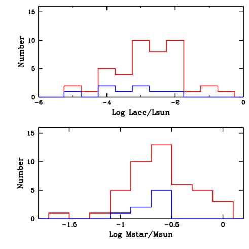
Figure 1: Accretion luminosity (top) and stellar mass (bottom) distribution. Red histogram for stars in Lupus, blue for stars in $\sigma$ Ori.

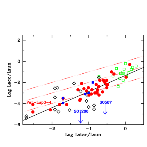
Figure 2: L_acc as function of L_star for objects in Lupus (red dots) and $\sigma$ Ori (filled blue squares). Open green squares plot the Taurus TTS of Gullbring et al. (1998); black diamonds the results of Herczeg & Hillenbrand (2008). The black line shows the best-fitting relation (GTO objects only) with slope 1.53; dashed lines are the locus L_acc/L_star=1, 0.1, 0.01 from top to bottom, respectively.

4 Results

Table 1: Observed Forbidden Lines

Element	$\chi_{ion}$	$\lambda_{vacuum}$	$\lambda_{air}$	Lower	Upper	$g_{1}$	$g_{2}$	Tex	A21	ncr	Number of detections
	(eV)	(nm)	(nm)	level	level			(K)	(s-1)	(cm-3)	Lupus	$\sigma$ Ori
O i	0	557.89	557.7339	${}^{1}D_{2}$	${}^{1}S_{0}$	5	1	48619	1.26	1.0e+8	28	4
O i	”	630.20	630.0304	${}^{3}P_{2}$	${}^{1}D_{2}$	5	5	22830	5.6e-3	1.8e+6	31	7
O i	”	636.55	636.3776	${}^{3}P_{1}$	${}^{1}D_{2}$	3	5	22830	1.8e-3	1.8e+6	25	5
O ii	13.618	372.98	372.8815	${}^{4}S^{0}_{3/2}$	${}^{2}D^{0}_{5/2}$	4	4	38574	2.0e-5	3.3e+3	3	4
O ii	”	372.71	372.6032	${}^{4}S^{0}_{3/2}$	${}^{2}D^{0}_{3/2}$	4	6	38603	1.8e-4	3.8e+3	9	3
O ii	”	732.22	731.89	$2D^{0}_{5/2}$	${}^{2}P^{0}_{3/2}$	4	6	58224	9.9e-2	1.3e+7	2	1
O ii	”	733.17	732.97	$2D^{0}_{3/2}$	${}^{2}P^{0}_{1/2}$	6	2	58121	8.7e-2	2.2e+6	2	1
S ii	10.360	407.75	407.6349	${}^{4}S^{0}_{3/2}$	${}^{2}P^{0}_{1/2}$	4	2	35430	7.7e-2	1.9e+6	8	2
S ii	”	406.98	406.8600	${}^{4}S^{0}_{3/2}$	${}^{2}P^{0}_{3/2}$	4	2	35354	1.9e-1	2.6e+6	21	5
S ii	”	671.83	671.644	${}^{4}S^{0}_{3/2}$	${}^{2}D^{0}_{5/2}$	4	6	21416	2.0e-4	1.7e+3	5	3
S ii	”	673.27	673.081	${}^{4}S^{0}_{3/2}$	${}^{2}D^{0}_{3/2}$	4	4	21370	6.8e-4	1.6e+4	11	3
N i	0	519.93	519.7902	${}^{4}S^{0}_{3/2}$	${}^{2}D^{0}_{3/2}$	4	4	27673	2.0e-5	2.2e+3	11	1
N i	”	520.17	520.0257	${}^{4}S^{0}_{3/2}$	${}^{2}D^{0}_{5/2}$	4	6	27660	7.6e-6	1.2e+3	1	1
N ii	14.534	654.99	654.805	${}^{3}P_{1}$	${}^{1}D_{2}$	3	5	22037	9.8e-4	8.5e+4	1	2
N ii	”	658.53	658.345	${}^{3}P_{2}$	${}^{1}D_{2}$	5	5	22037	2.9e-3	8.5e+4	13	2

Table 2: Kinematical Components: ”L”: LVC; ”Hb”: blue-shifted HVC; ”Hr”: red-shifted HVC.

Name	[O i]	[O i]	[S ii]	[S ii]	[O ii]	[N ii]
	557.73	630.03	406.86	673.08	372.60	658.34
Sz66	L	L	L	L	L	L
AKC2006-1	-	-	-	-	-	-
Sz69	L	L,Hb,Hr	L,Hb	Hb,Hr	Hr	Hb,Hr
Sz71	L	L	-	-	-	-
Sz72	L	L,Hb	Hb	Hb	Hb	-
Sz73	L	L,Hb	Hb	Hb	Hb	Hb
Sz74	L	L	-	-	-	-
Sz84	L	L	-	-	L	-
Sz130	L	L,Hb	Hb	-	-	Hb
Sz88A	L	L	L	-	-	-
Sz88B	L	L	L	-	-	-
Sz91	L	L	-	-	-	-
Lup713	-	-	-	-	-	-
Lup604s	-	L	-	-	-	-
Sz97	-	L	-	-	-	-
Sz99	L	L,Hr	Hr	Hr	-
Sz100	L	L,Hb,Hr	L,Hb	L,Hb	Hb	Hb
Sz103	L	L	L	L	-	Hb
Sz104	L	L	-	-	-	-
Lup706	-	-	-	-	-	-
Sz106	L	L	L	L	L	L
Par-Lup3-3	-	L	-	-	-	-
Par-Lup3-4	L	L	L	L	L	L
Sz110	L	L	L	-	-	-
Sz111	L	L	-	-	-	-
Sz112	L	L	L	-	-	-
Sz113	L	L,Hb	Hb	Hb	-	Hb
J160859	L	L	L	-	-	-
c2dJ1609	L	L	L	-	-	L
Sz114	L	L,Hb	L	-	-	-
Sz115	-	-	-	-	-	-
Lup818s	L	L	-	-	-	-
Sz123A	L	L,Hb	L,Hb	-	-	Hb
Sz123B	L	L,Hb	L,Hb	-	-	Hb
SST-Lup3-1	-	-	-	-	-	-
SO397	-	-	-	-	-	-
SO490	L	L	-	-	-	-
SO500	-	L,Hb	-	-	-	-
SO587	-	L	L	L	L	L
SO646	-	L	L	-	-	-
SO848	L	L,Hb	Hb	L,Hb	L	L,Hb
SO1260	L	L	L	-	-	-
SO1266	L	L	Hb	L	Hb	-

We have searched the spectra of our targets for evidence of emission in the forbidden lines of O i, O ii, O iii, S ii, S iii, N i, N ii, C i, Ca ii in the blue, visual and near-IR wavelengths. The lines detected are [O i] 557.79, the O i doublet at 630.03, 636.37nm, the O ii doublets at 372.88, 372.60nm and 731.89, 732.97nm, the S ii doublets at 407.63, 406.86nm and 671.64, 673.08nm, the N ii doublet at 654.80, 658.34nm. The [N i] 519.79nm is detected in many objects, but it is contaminated by Fe lines that cannot be reliably deconvolved at the resolution of our spectra, so that its intensity is very uncertain. In few cases, we detect also the [N i] 346.649, 346.654 doublet, but in this spectral region the signal-to-noise ratio achieved is generally very low; there are no detections of the N i quadruplet around 1 micron. In Par-Lup3-4, which has the richest emission line spectrum, we detect also the [Ca ii] 729.15nm, [C i] 982.40, 985.30nm lines and the S ii quadruplet at $\sim$1030nm. In addition, there are some lines of Fe in different ionization states (Giannini et al., 2013).

Table 1 lists the spectroscopic parameters of the lines. For each line, it gives the ionization potential of the ion, the line wavelength in the vacuum and in air, the quantum number and multiplicity of the lower and upper state, the excitation temperature of the upper state of the transition, the value of the A₂₁ coefficient, the critical density for collisions with electrons and the number of stars in which the line is detected. The emissivity of the lines used in this paper have been kindly provided to us by Bruce Draine and computed using a 5-level atomic model with collisional rates for electrons or atomic hydrogen (Draine, 2011).

Some lines are detected in a large fraction of stars, for example the [O i] 630.03nm (detected in 38/44 stars) or the [S ii] 406.98nm which is detected in 26/44 stars; in 6 stars (AKC2006-1, Lup713, Lup706, Sz115, SST-Lup3-1, SO397) no forbidden line is detected. Some lines of ions with high ionization potential, such as the [N ii] 658.34  are also seen in several stars.

There is a large variation in the number of forbidden lines detected in different stars. None of the low luminosity and low accretion luminosity objects show a rich forbidden line spectrum, with the exception of four objects (Par-Lup3-4, SO587, SO848 and SO1266), that will be discussed in more detail in the following.

Of the stars with no forbidden line detections, 4 (AKC2006-1, Lup713, Lup706, SST-Lup3-1) are among the low luminosity, low L_acc objects, while 2 (Sz115 and SO397) are typical TTS and the lack of lines is somewhat surprising. Note, however, that in all cases the upper limits to the line luminosities are of the order of the detections, not significantly lower.

5 Line Profiles

Forbidden lines from TTS are known to show multiple components. Typically, one can identify a low-velocity component, broad and roughly symmetric, with a slightly blue-shifted peak velocity, and high-velocity components, with peaks shifted to the blue and/or to the red (much less frequently) by tens of km/s.

We have examined the lines [O i] 630.03, [O i] 557.79, [S ii] 406.86, [S ii] 673.08, [O ii] 372.60, [O ii] 731.89 and [N ii] 658.34 and classified them as high-velocity blue-shifted (HVC-blue), high-velocity red-shifted (HVC-red) and low-velocity (LVC) components.

Because the spectral resolution of X-Shooter is relatively low, we have adopted a conservative criterion to identify the presence of a HVC component in each line: i) when a line has a single component shifted by more than $\pm 40$ km/s this is identified as an HVC; ii) when more than one component is present the HVC is identified if it is well resolved from the LVC; iii) when a line shows a broad wing, this wing is identified as an HVC if another line has an HVC at the same velocity defined by one of the previous criteria. In Table 2 we report the components identified in each line for all stars in our sample. In this Table “L” stands for LVC, “Hb” for HVC-blue, and “Hr” for HVC-red. LVC and HVC components are clearly detected in several objects. The star Sz83 (RU Lup) has very complex line profiles, not only for the forbidden lines but also for the permitted lines that trace directly the accreting matter (Alcalá et al., 2014), and will not be discussed in this paper.

Our criteria in classifying the different components differ from those adopted by Hartigan et al. (1995). These authors define the LVC as the portion of the spectrum between -60 and +60 km/s and measured the HVC as the total flux (integrated over all the profile) minus the LVC flux. Note also that the spectral resolution they used is about 12 km/s, which allowed them a better definition of the line wings.

We compute the intensity and the peak velocity of each component by fitting a gaussian profile to the line. Table LABEL:tab_tabellone_1, LABEL:tab_tabellone_2, LABEL:tab_tabellone_3 and LABEL:tab_tabellone_4 give for each star the properties (flux, uncertainty, peak velocity and FWHM) of each component for the set of lines defined above. Upper limits ($3\sigma$) have been computed from the rms of the continuum, assuming a line FWHM width of 50 km/s ($3{\rm rms}\times FWHM/\sqrt{\rm(nres)}$, where ${\rm nrs}$ is the number of resolution elements within 50 km/s). The uncertainty on $V_{peak}$ is $\sim$$10$ km/s. Figure 3 shows the distribution of the peak velocity; almost all LVC have a blue-shifted peak, with $V_{peak}$ smaller than $\sim 20$ km/s. Note that the gaussian fit tends to overestimate $V_{peak}$ if there is a significant unresolved asymmetric wing. In general, our values of $V_{peak}$ are consistent, given the resolution of our spectra, with the typical value $\sim 5$ km/s of Hartigan et al. (1995). The large majority of the lines, both LVC and HVC, are broad and well resolved, with FWHM ranging from the resolution limit to $\mathbin{\lower 3.0pt\hbox{$\hbox to0.0pt{\raise 5.0pt\hbox{$\char 62\relax$}\hss}\mathchar 29208\relax$}}100$ km/s.

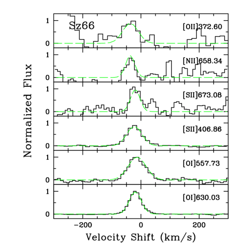
Figure 13: Normalized, continuum subtracted line profiles (as labelled) for the object Sz66. In this and the following figures the dashed colored curves show the LVC (green), HVC-blue shifted (blue) and HVC red-shifted (red); the total is given by the dotted (black) line. In this object, only the LVC is detected.

Examples of the observed line profiles are shown in Appendix C. Fig 12 shows the observed profiles of the [O i] 630.03 line for all the GTO objects. Fig. 13 – 21 show line profiles for a selection of objects where several lines were detected, together with the results of the gaussian fitting and deconvolution.

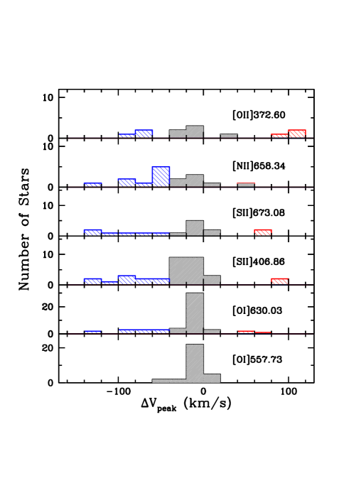
Figure 3: Distribution of the peak velocity shift with respect to the star (solid for LVC, hatched blue for HVC-blue, red for HVC-red) for different lines, as labelled.

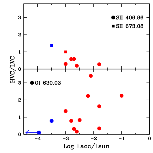
Figure 4: Ratio of the HVC to the LVC intensity in objects where both components are simultaneously detected. The bottom panel refers to the [O i] 630.03 lines; the top panel to the [S ii] 406.86— and [S ii] 673.08 lines, as labelled. Red and blue for Lupus and $\sigma$ Ori, as before.

5.1 Statistics

For each star, Table 2 characterizes the profile of the lines discussed in the following. LVC, HVC-blue and/or HVC-red may be present in all the lines we observe; as also shown by previous studies, the HVC-red is very rare. The exception is the [O i] 557.79 that does not show any HVCs clearly identifiable in our spectra, although in some cases there is a hint of emission in the line wings that could be resolved as a separate component in higher sensitivity and resolution spectra. This is in agreement with the results of other authors (i.e. Hartigan et al., 1995; Rigliaco et al., 2013).

When detected, the [O i] 630.03 always has a LVC, while a HVC is detected in 12/37 of cases. In general, HVCs are detected proportionally more often in high excitation/high ionization lines such as [N ii] 658.34 and [O ii] 372.60, or in lines with low critical density, such as the [S ii] 673.08 doublet.

Of particular interest are stars where both LVC and HVC are detected, since in these cases the potential confusion between the LVC emission and that of a jet projected on the plane of the sky does not exist. Our sample includes 12 stars with both LVC and HVCs in the [O i] 630.03 line; of these, 5 show both components also in the [S ii] 406.86 line and 2 in the [S ii] 673.08 one. The intensity ratio between the two components is shown in Figure 4 for the [O i] 630.03, [S ii] 406.86 and [S ii] 673.08 lines. The ratios range from very small to $\sim 3.5$; however, only few objects have a very strong HVC (high value of the ratio), and in most cases the HVC has intensity lower than that of the LVC.

5.2 Contamination of the LVC sample by HVC in the plane of the sky

When only one component with small peak velocity is detected in any given object, it is possible that, rather than a bona-fide LVC, it is a HVC misclassified because of projection effects.

This is certainly the case of Par-Lup3-4, which has a well resolved jet and an edge-on disk obscuring the central star so that both its stellar and its accretion luminosity are largely underestimated (Bacciotti et al., 2011; Alcalá et al., 2014). At the spatial resolution of our spectra ($\sim 1$ arcsec, due to seeing), forbidden lines from Par-Lup3-4 have very small $V_{peak}$ and we classify them as LVC. Contrary to many other cases, however, the three lines [S ii] 673.08, [O ii] 372.60 and [N ii] 658.34  are quite strong in this object, with ratios to the [O i] 630.03 line of 0.3, 0.1 and 0.05, respectively.

Two additional objects in Lupus also have a rich LVC spectrum, with all the lines clearly detected. They are Sz66 and Sz106. The high-excitation lines are particularly strong, with ratios [O ii] 372.60/[O i] 630.03 and [N ii] 658.34/[O i] 630.03 of 0.02 and 0.05 for Sz66 and 0.25 and 0.3 for Sz106. For the latter object there is evidence in the literature for an edge-on geometry (Comerón et al., 2003; Alcalá et al., 2014). It is probable that, as in Par-Lup3-4, we are detecting the emission of a jet with axis close to the plane of the sky.

The presence of 3 ”spurious” LVC objects in Lupus (about 10%) is consistent with the expectations for a randomly oriented sample. Assuming a velocity of 200 km/s for the HVC (e.g. Appenzeller & Bertout, 2013), we expect that about 12% have projected velocities less than $\sim 40$ km/s and would therefore be classified as LVC in our analysis.

Given the small number of potentially spurious LVC, we include all the objects in the GTO sample in the following analysis (with the already noted exception of Sz83).

5.3 Doublets

All the lines in our sample are doublets, with the exception of the [O i] 557.79. In some cases (i.e., the [O i] 630.03 and the [N ii] 658.34 doublets), the ratio of the intensity of the two components depends on atomic parameters only; in others, it depends also on the physical conditions that determine the level population. If, for example, electronic collisions dominate, the intensity ratio depends on the electron density and, to a lower degree, on the temperature, as for the [S ii] 406.86 and [S ii] 673.08 case. The range, however, is not large. The [S ii] 673.08 ratio ranges from $\sim 1.5$ for density much lower than the critical density, to $\sim 0.5$ in the high density limits. In the case of the [S ii] 406.86 doublet, the [S ii] 407.63 is always weaker than the [S ii] 406.86, with a ratio of $\sim 0.3$ for $n_{e}\ll n_{cr}$ to $\sim 0.2$ in the high-density limit. Our observed ratios and upper limits are always consistent with the predictions. Unfortunately, the large errors, especially on the weaker components, prevent us from using these line ratios to constrain the density of the emitting regions.

6 The Low-Velocity Component

In the following, we will focus our discussion on the region emitting the LVC and on its properties.

6.1 Line Intensities

Figure 5 shows the luminosity of the LVC of the lines [O i] 630.03, [O i] 557.79 as function of L_star (left panels) and L_acc (right panels).

For the two O i lines, which are detected in a large fraction of objects, there is an excellent correlation of L_line with both L_star and L_acc, with similar slopes for the two lines; using ASURV, EM method (Feigelson & Nelson, 1985), we find:

$$LgL({O\textsc{i}}\,630.03)=(1.37\pm 0.18)LgL_{star}+(-4.56\pm 0.18)$$ (1)

$$LgL({O\textsc{i}}\,630.03)=(0.81\pm 0.09)LgL_{acc}+(-3.66\pm 0.27)$$ (2)

$$LgL({O\textsc{i}}\,557.79)=(1.37\pm 0.16)LgL_{star}+(-5.00\pm 0.16)$$ (3)

$$LgL({O\textsc{i}}\,557.79)=(0.79\pm 0.07)LgL_{acc}+(-4.13\pm 0.20)$$ (4)

Upper limits to the line luminosity are taken into account. We have not included in the correlations the object Par-Lup-3-4, because of its very uncertain values of L_star and L_acc, and, in the case of the correlations with L_acc, the two objects in $\sigma$ Ori which have only L_acc upper limits. If they are included, the correlations will be slightly flatter.

Figure 5 plots also the observed [O i] 630.03 and [O i] 557.79 luminosities for other stars in the literature. The black crosses, in particular, are values for DR Tau at different epochs; stellar, accretion and line luminosities have been obtained from X-Shooter spectra in the same manner as the objects analyzed in this paper (Banzatti et al., 2014). The green points refer to the sample of TTS in Taurus firstly studied by Hartigan et al. (1995), but with extinction, L_star and L_acc as re-measured by Gullbring et al. (1998). The black diamonds are the low-mass objects studied by Herczeg & Hillenbrand (2008), corrected according to the new values of extinction, L_star and L_acc given by Herczeg & Hillenbrand (2014), when available.

The correlations of eq.(1)–(4) describe quite accurately also the higher luminosity TTS from the literature. The slope of the L_line-L_acc correlation for the [O i] 630.03 line is similar within the uncertainties to that of Herczeg & Hillenbrand (2008). On the other hand, it is marginally steeper than the slope ($0.52\pm 0.07$) found by Rigliaco et al. (2013) using the [O i] 630.03 LVC luminosities of Hartigan et al. (1995) and new determinations of L_acc from the H$\alpha$ luminosity. Inspection of Figure 5 shows that in the TTS sample alone (green squares) L([O i] 630.03) has a flat dependence on L_acc, and it is possible that the discrepancy comes from the different range of L_acc covered by the two samples. The possibility of a change of the slope at high L_acc is also suggested by the location of DR Tau (black crosses); however, there are differences in the quality of the data and in the methods used to determine stellar and accretion properties for the various samples that prevent any conclusion at this stage.

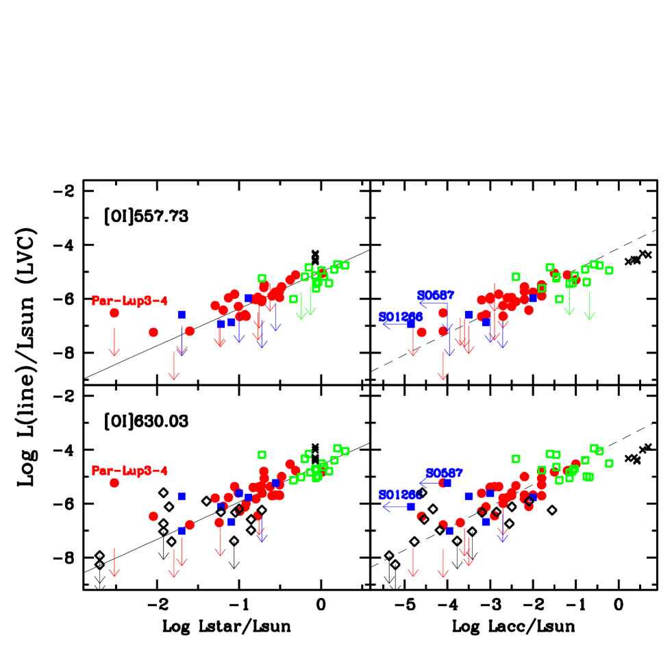
Figure 5: Line luminosities for the [O i] 630.03 and [O i] 557.79 are plotted as function of the stellar luminosity (left Panels) and of the accretion luminosity (right Panels). Red filled dots are the Lupus objects, blue filled squares are objects in $\sigma$ Ori; arrows show 3$\sigma$ upper limits. The black crosses show the same quantities for the strongly accreting TTS DR Tau at different epochs (Banzatti et al., 2014). Black diamonds are values for Taurus very low mass objects from Herczeg & Hillenbrand (2008, 2014, see text); green open squares denote Taurus TTS from Gullbring et al. (1998) and Hartigan et al. (1995), as described in the text. Few objects discussed in § 6.2 are labelled in some panels only, to avoid confusion.

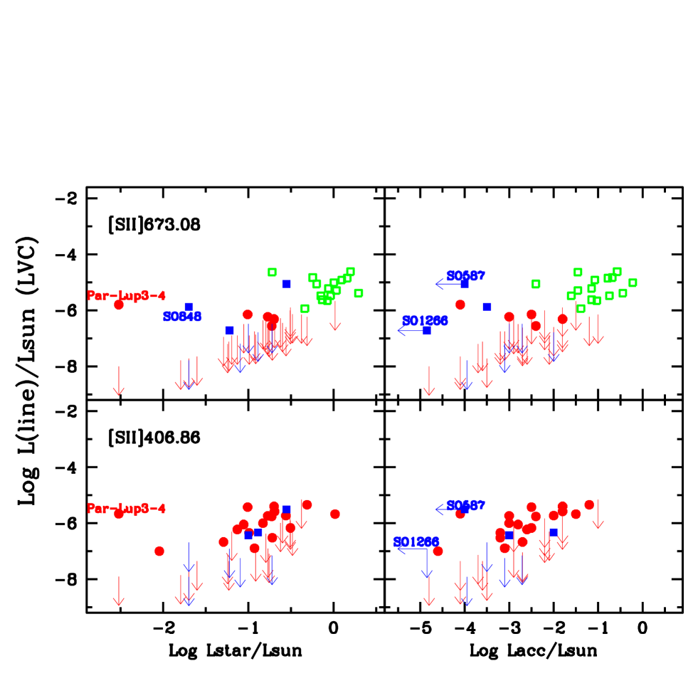
Figure 6: Line luminosities for the [S ii] 406.86 and [S ii] 673.08 lines are plotted as function of the stellar luminosity (left Panels) and of the accretion luminosity (right Panels). Red dots are the Lupus objects, blue filled squares are objects in $\sigma$ Ori; arrows show 3$\sigma$ upper limits. Green open squares show the position of Taurus TTS from Gullbring et al. (1998) and Hartigan et al. (1995), as described in the text.

As mentioned in § 3, in the GTO objects there is a rather tight correlation between L_star and L_acc. This makes it very difficult to identify which of the system properties controls the emission of the forbidden lines, either the stellar or the accretion ones. It is interesting that the relation to L_acc is almost linear, as for all the permitted lines that are tracers of the accretion process (Alcalá et al., 2014).

Figure 6 plots the luminosity of the [S ii] 406.86 and [S ii] 673.08 lines as function of L_star and L_acc  respectively. As for the O i lines, there is a good correlation with both, with similar slopes, but with a larger number of upper limits, especially in the [S ii] 673.08 lines.

6.2 Individual Objects

There are few objects that deviate significantly from the general trends, and we have identified them in the figures. In addition to Par-Lup3-4, that we have already discussed, there are 2 stars in $\sigma$ Ori with very strong forbidden lines. One is SO587 which has an upper limit to L_acc $\sim 10^{-4}$ L_⊙, and a LVC spectrum with especially strong high-excitation lines, i.e., [S ii] 673.08/[O i] 630.03$\sim 1.5$, [N ii] 658.34/[O i] 630.03$\sim 1.7$ and [N ii] 658.34/[O i] 630.03$\sim 3$. Also the [S ii] 406.86 line is very strong for the observed L_acc (but not for the L_star of the object). No [O i] 557.79 is detected. This object has been studied by Rigliaco et al. (2009), who interpreted it as a photoevaporative wind heated by the nearby O9.5 star $\sigma$ Ori. The physical conditions in the outer wind should therefore be different from those in similar objects where no hot nearby star is present, explaining the strong emission in the high-excitation lines.

Another object in $\sigma$ Ori has a rich spectrum of forbidden lines, namely SO848. In this case both a LVC and a HVC-blue are detected and the LVC luminosities are as expected, given the L_star and L_acc of the object. The only exception is the [S ii] 673.08 line, which is unusually strong. It is possible that the presence of the hot star $\sigma$ Ori affects at some level also the emission of SO848, which has a projected distance from $\sigma$ Ori of 0.45 pc (to be compared with 0.35 for SO587). A deeper analysis of this aspect, however, requires line profiles of higher spectral resolution, that will allow a more accurate component separation and also the identification of the spectral profiles typical of photoevaporated winds heated by an external source (see, e.g., Rigliaco et al., 2009).

SO1266 is a low luminosity object in $\sigma$ Ori, with only an upper limit to L_acc from continuum excess measurement (Rigliaco et al., 2012); it has relatively strong emission lines of H and Ca ii, so that the mass accretion rate derived from the relation between line luminosity and L_acc would be about ten times higher than the continuum upper limit. Rigliaco et al. (2012) argue that chromospheric emission contributes about 80% of the line emission (see also Manara et al., 2013). We detected LVC of [O i] 630.03, [O i] 557.79 and [S ii] 673.08  which are stronger than in other objects with similarly low L_acc, but not when compared to other objects with similar L_star. This is an interesting object, that needs follow-up studies.

6.3 Physical conditions in the LVC emitting region

Line ratios provide very interesting information on the physical conditions of the emitting region. Figure 7 top Panel plots the values of the ratio of the two [O i] lines at 557.73 and 630.03 as function of L_acc for the GTO sample and for the more luminous TTS from the literature described in the previous section. The ratio is impressively constant over the whole sample, with values ranging from $\sim 0.1$ to $\sim 1$. There is no correlation with either the L_star or the intensity of the [O i] 630.03 line. This is very similar to what has been found by Hartigan et al. (1995) for higher luminosity TTS, also shown in the figure.

The observed values can be compared in Figure 7, bottom panel, to the predictions of homogeneous and isothermal models where the excitation is due to electron collisions (solid curves, bottom axis) or to collisions with neutral hydrogen (dashed curves, top axis). Different curves correspond to different temperatures, as labelled. Note that the model predictions for the intensity of the [O i] 557.79 when collisional excitation by H dominates are uncertain, as the de-excitation cross section of the level ${}^{1}S_{0}$ is not known. The calculations in Figure 7 have been performed assuming the same rate of the $1D_{2}$ level (see also the discussion in Gorti et al., 2011). The grey area shows the location of the observed ratios; one can see that, unless the temperature is significantly higher than $10^{4}$, they are consistent with a rather dense gas, with $n_{e}\gg n_{cr}$([O i] 630.03) $\mathbin{\lower 3.0pt\hbox{$\hbox to0.0pt{\raise 5.0pt\hbox{$\char 62\relax$}\hss}\mathchar 29208\relax$}}10^{7}$ cm^-3, or, alternatively, $n_{H}\gg 10^{10}$ cm^-3, if collisions with H dominate the level excitation. We have limited our models to $T\leq 10^{4}$ K, but we note that at the high temperature $T=30000$ K, $n_{e}=10^{5}$ cm^-3, the ratio [O i] 630.03/[O i] 557.79  is only $\sim 0.1$ barely consistent with the low end of the observed interval, and would decrease further for lower values of $n_{e}$. Temperatures below $\sim 5000$K cannot reproduce the observed ratios, no matter the value of the density. In the following, we will assume that the region emitting the [OI] lines have density $n_{e}\geq 10^{7}$ cm^-3 (or $n_{H}\geq 10^{10}$ cm^-3) and temperature $5000\leq T\leq 10000$K.

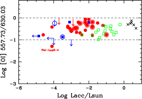
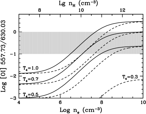
Figure 7: Top Panel: Ratio [O i] 557.79/[O i] 630.03 as function of L_acc for stars in Lupus (red dots) and $\sigma$ Ori(filled blue squares). Arrows indicate 3$\sigma$ upper limits. Objects where both a LVC and a HVC are detected are marked by large open circle. Black crosses show the values for the set of DR Tau spectra obtained at different epochs, green open squares are stars in Taurus (see text). Bottom Panel: Model predictions for collisions with electron (solid curves) and with hydrogen atoms (dashed curves). Different curves refer to different temperatures, as labelled. The $n_{e}$ scale is shown in the bottom axis, that for $n_{H}$ on the top axis. The grey area shows the location of the observed values, marked by the two dashed lines in the top panel.

The third most frequently observed line is [S ii] 406.86. Figure 8, top panel plots the observed ratio of the intensity of the [S ii] 406.86 to [O i] 630.03 line as function of L_acc. We have marked the objects where there is unambiguous evidence that the two lines form in the LVC, i.e., both LVC and HVC are detected in the [O i] 630.03 line, as detailed in § 5.1. Figure 8, bottom panel plots the predictions for electronic collisions (solid curves) and atomic hydrogen collisions (dashed curves; same as Figure 7). The [S ii] 406.86 line has a critical density for electronic collisions very similar to that of the [O i] 630.03 line and a difference in the energy of the upper level of $\sim 10000$ K only, so that their ratio is expected to vary little with the density and temperature of the emitting region. We have assumed that all oxygen is neutral, all solphur is S ii and the Asplund (2005) solar elemental abundances ( $\alpha$(O)$=4.5\times 10^{-4}$, $\alpha$(S)$=1.4\times 10^{-5}$). The ratio S/O is very similar if we take, instead, the proto-solar abundances of Lodders (2003). The results in the case of collisions with neutral hydrogen are very uncertain, as no de-excitation rates for collisions with neutral hydrogen exist. The curves in the bottom panel of Figure 8 have been computed in the orbiting collision approximation (see eq. 2.34 of Draine (2011).

For the density and temperature values that account for the observed [O i] 630.03/[O i] 557.79 ratios, the models predict ratios [S ii] 406.86/[O i] 630.03$\sim$0.2-0.5. This interval is shown by the dashed horizontal lines in the top panel and the dark-shaded region in the bottom panel. About 65% of the measured values (and 5/6 of those with both components) lie in this interval, only 3 objects have ratios higher than 0.5, while 5 measurements plus 5 upper limits are lower than 0.2. In the objects within the dark grey region, the strength of the [S ii] 406.86 line is therefore as expected if the three lines [O i] 630.03, [O i] 557.79 and [S ii] 406.86 are emitted by the same region and are the result of thermal processes, namely collisional excitation. We note also that this emitting region cannot be much ionized. As the oxygen ionization is coupled to that of hydrogen by charge exchange, an ionization fraction $n_{e}/n_{H}\sim 0.5$, for example, would shift all model predicted ratios upward by 0.3 dex, i.e., above the observed range. Moreover, if O ii/O i $\sim 0.5$, the [O ii] 731.89 line should have an intensity comparable to that of the [O i] 557.79, while it is detected in very few objects (Table 1). Neither of these is a strong quantitative argument, but, all together, it seems likely that in these objects the LVC emitting region is mostly neutral.

Very few objects have ratios [S ii] 406.86/[O i] 630.03 larger than $\sim 0.5$; in these cases, it is possible that a significant fraction of oxygen is ionized. The largest ratio is observed in Sz106, where we detect also the [O ii] 372.60  and [N ii] 658.34 lines at roughly zero velocity, and which is likely an object where the forbidden line emission is dominated by a jet aligned with the plane of the sky, where the ionization fraction (and therefore the ratio O ii/O ) could be of 20-30% (Bacciotti and Eislöffel, 1999). Note, however, that the large values of the observed [S ii] 406.86/[O i] 630.03 ratio ($\sim 1.6$) requires an ionization fraction $n_{e}/n_{H}\mathbin{\lower 3.0pt\hbox{$\hbox to0.0pt{\raise 5.0pt\hbox{$\char 62\relax$}\hss}\mathchar 29208\relax$}}0.5$.

Observed [S ii] 406.86/[O i] 630.03  below $\sim 0.2$ are difficult to explain if the line emission is thermal, even when the rather large errors of the observed points are taken into account. One would need to assume that a significant fraction of sulphur is either neutral or doubly ionized, which seems unlikely, or that the temperature is significantly lower than 5000 K, which is inconsistent with the constraints obtained from the [O i] 557.79/[O i] 630.03 ratio. In these objects, it is possible that a dominant part of the O i emission is due to non-thermal processes, namely photodissociation of OH, as advocated for TW Hya by Gorti et al. (2011); we will go back to this point in § 7.2.

A LVC [S ii] 673.08 is detected in few GTO objects. This line has a critical density much lower than either the [S ii] 406.86 or the [O i] 630.03 lines and is relatively stronger in lower density regions. Figure 9, top panel plots the [S ii] 673.08/[S ii] 406.86 ratio as function of L_acc, and Figure 9, bottom panel the predictions of the models. The ratios tend to be higher than expected for the physical conditions that account for the [O i] 630.03/[O i] 557.79 and [S ii] 673.08/[O i] 630.03 intensity ratios, suggesting that a region of lower electron density (but still higher than $\sim 10^{5}$ cm^-3) is emitting most of the [S ii] 673.08 line. The two sources with the highest ratios [S ii] 673.08/[S ii] 406.86 are Par-Lup3-4 and SO587, that we have already discussed.

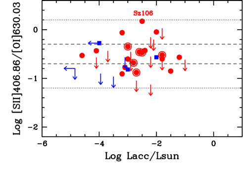
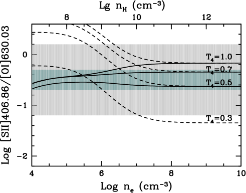
Figure 8: Same as Figure 7 for the ratio [S ii] 406.86/[O i] 630.03. In the bottom Panel, the dark-grey area shows the location of 65% of the observed values (dashed lines in the top panel). Three points lie in the upper ligh-grey area, the rest in the lower light-grey one (dotted lines in the top panel).

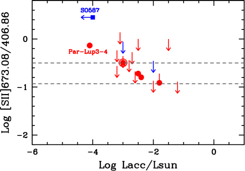
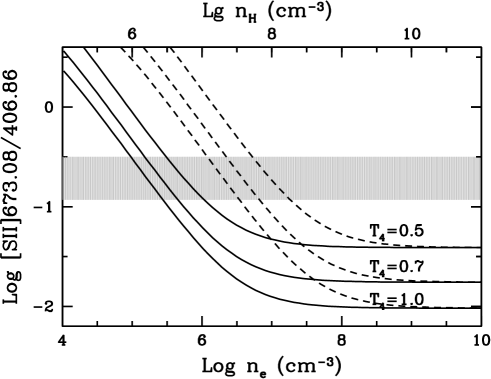
Figure 9: Same as Figure 7 for the ratio of the LVC [S ii] 673.08/[S ii] 406.86. The shaded region in the bottom panel shows the locus of the four detections in the upper panel (excluding the special cases of Par-Lup3-4 and SO587, see text), between the two dashed lines in the top panel.

6.4 Mass, Momentum and Volume

The analysis of the O i and S ii lines in the previous section indicates that in 65% of the objects we have evidence that the emission is coming from a warm ($T\sim 5000-10000$ K), dense ($n_{e}\mathbin{\lower 3.0pt\hbox{$\hbox to0.0pt{\raise 5.0pt\hbox{$\char 62\relax$}\hss}\mathchar 29208\relax$}}10^{6}$ cm^-3), mostly neutral gas. As the density is larger than the critical density, the mass of gas in the emitting region can be derived from the luminosity of any forbidden line and is function of the temperature only. If we consider the [O i] 630.03 line, which is detected in the largest number of stars, it is:

$$M_{gas}=\mu m_{H}{{L({\rm[{O\textsc{i}}]\,630.03})}\over{j({\rm[{O\textsc{i}}]\,630.03})\,\alpha({O\textsc{i}})}}$$ (5)

where $\mu m_{H}=2\times 10^{-24}$ is the mean molecular weight of neutral gas, L([O i] 630.03) is the line luminosity, $j({\rm[{O\textsc{i}}]\,630.03})$ is the line emissivity and $\alpha({O\textsc{i}})$ is the fractional abundance of neutral oxygen. For $T\sim 5000-10000$ K, in the high density limit $j({\rm[{O\textsc{i}}]\,630.03})$ ranges from $1.2\times 10^{-16}$ to $1.1\times 10^{-15}$ erg s^-1 per O i atom. Assuming an average value $\sim 6\times 10^{-16}$ and that most oxygen is O i, it is:

$$M_{gas}\sim 1.4\times 10^{-11}M_{\odot}\big{(}{{L({\rm[{O\textsc{i}}]\,630.03})}\over{10^{-6}\,\rm L_{\odot}}}\big{)}$$ (6)

In the GTO sample, $M_{gas}$ increases from $\sim 1.4\times 10^{-12}$ for the lowest luminosity objects (L([O i] 630.03)/L_⊙=$10^{-7}$) to $\sim 1.4\times 10^{-9}$ M_⊙ for the objects with the strongest [O i] 630.03. The corresponding momentum, assuming a velocity $V_{peak}\sim 10$ km/s, goes from $\sim 1.4\times 10^{-11}$ to $\sim 1.4\times 10^{-8}$ M_⊙ km/s.

The volume occupied by the emitting gas can also be derived from the line luminosity if the gas density is known:

$$Vol_{gas}=\big{(}{{L({\rm[{O\textsc{i}}]\,630.03})}\over{n_{H}\,j({\rm[{O\textsc{i}}]\,630.03})\,\alpha({O\textsc{i}})}}\big{)}$$ (7)

If electron collisions dominate the level excitation, we can derive a very conservative upper limit of $n_{H}\sim$$10^{8}$ cm^-3, assuming $n_{e}\sim$$10^{7}$ cm^-3 and an ionization fraction $\sim$$0.1$. The minimum $n_{H}$ will be at least hundred times higher if atomic hydrogen collisions dominate. Therefore, $Vol_{gas}$ ranges from $\mathbin{\lower 3.0pt\hbox{$\hbox to0.0pt{\raise 5.0pt\hbox{$\char 62\relax$}\hss}\mathchar 29208\relax$}}1.4\times 10^{37}$ cm³ for objects with L([O i] 630.03)$\sim$$10^{-7}$ L_⊙ to $\mathbin{\lower 3.0pt\hbox{$\hbox to0.0pt{\raise 5.0pt\hbox{$\char 62\relax$}\hss}\mathchar 29208\relax$}}1.4\times 10^{40}$ cm³ when L([O i] 630.03)$\sim$$10^{-4}$ L_⊙. This would translate in a linear dimension of 0.16 AU to 1.6 AU, assuming spherical geometry.

The values of the mass of the dense, warm gas and the maximum values it occupies are plotted in Figure 10 as function of the mass of the central object.

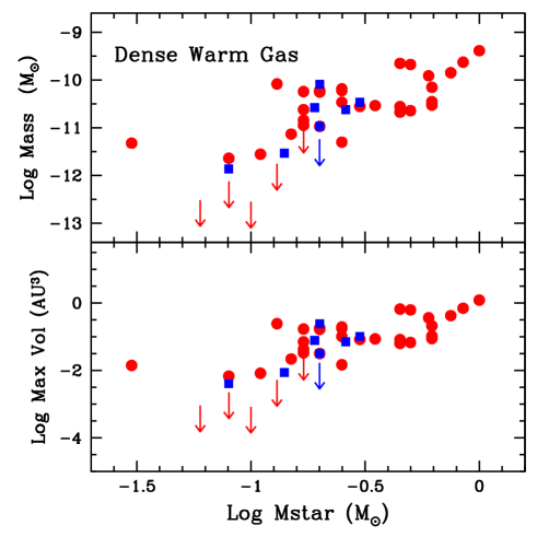
Figure 10: Properties of the dense, warm gas as function of the stellar mass for the GTO sample. Red dots are objects in Lupus, blue filled squares in $\sigma$ Ori; arrows are objects with upper limits of the [O i] 630.03 luminosity, from which we derive the properties of the emitting region. The top panel plots the mass of the gas in the region, the bottom panel the upper limit to the volume, computed for an electron density $n_{e}=10^{7}$ cm^-3, ionization fraction 0.1 ($n_{H}=10^{8}$ cm^-3). In both panels we have assumed a line emissivity which is the average between the values for T=10000 K ($1.1\times 10^{-15}$ erg $s^{-1}$ per O i) and T=5000 K ($1.2\times 10^{-16}$ erg $s^{-1}$ per O i) once $n_{e}\gg n_{cr}$.

7 Discussion

The small, blue-shifted velocity of the LVC line peaks is the main indication of their origin in a wind, ejected from the disk surface with low velocity (see Hartigan et al., 1995). The quality of our spectra does not allow us to constrain the peak velocity to an accuracy better than $\sim 10$ km/s, but the blue-shifts are clearly detected in all lines, and we will therefore discuss their properties in the context of the wind models.

7.1 Mass-loss rate

The mass-loss rate is the fundamental global quantity that characterizes the mass-loss process and its inpact on the disk evolution. All the existing estimates of $\dot{M}_{loss}$ have been derived for the HVC (Hartigan et al. (1995);see Cabrit (2002) for a discussion) and do not necessarily apply to the outflowing gas traced by the LVC emission, which can trace a different mechanism of mass-loss.

In spite of the number of spectroscopic data on the LVC, deriving a meaningful mass-loss rate is difficult, as different assumptions on the geometry of the ouflowing matter lead to very different estimates. A crude estimate of $\dot{M}_{loss}$ can be obtained by dividing the mass of the emitting region (eq.(6)) by a timescale $\tau=L/{\rm v}$ where $L$ and ${\rm v}$ are measured along the flow direction. Let us assume ${\rm v}\sim V_{peak}$, and the maximum value of the volume occupied by the emitting matter derived in § 6.4. Values of $\dot{M}_{loss}$ obtained assuming an outflow spherical geometry are in the range $\sim 2\times 10^{-11}-10^{-9}$ M_⊙/yr, approximately bewteen 1 and 0.1 $\dot{M}_{acc}$. If the outflow is lounched from a disk area $A$ in the vertical direction and has a cylindrical geometry, then $L=Vol/A$. We have considered two possibilities. The first is that the outflow is emitted by a disk annulus at a distance from the star such that the keplerian velocity $V_{kepler}=V_{peak}$; assuming an annulus width $\Delta R/R$=0.1, we find that $L$ is typically 10-30 times smaller than before and $\dot{M}_{loss}$$\gg$ $\dot{M}_{acc}$. The second possibility, suggested by models of photoevaporative winds, is that the emitting region is at a distance from the star of $\sim 1.8$ (M_star/M_⊙) AU (Alexander et al., 2014). In this case $L$ and $\dot{M}_{loss}$ are similar to those obtained for spherical geometry.

In fact, it is likely that $L$ is much larger than our estimates. If the flow velocity is not orthogonal to the disk, but has a large tangential component, as in a conical wind, then $L$ can be much larger and is defined by a change in the physical conditions, density in particular, that are traced by the forbidden lines we observe. A detail study of high-spectral and spatial resolution line profiles is needed to obtain an estimate of the mass-loss rate of the slow wind component.

7.2 Wind models

MHD disk winds have been associated to the LVC of the TTS forbidden lines (Kwan & Tademaru, 1995), as at their base, when the disk material becomes unbound, they have high density and low velocities (see, e.g., . (Ferreira et al., 2006; Suzuki & Inutsuka, 2009; Bai & Stone, 2013; Zanni & Ferreira, 2013; Lesur et al., 2013; Fromang et al., 2013; Bai, 2014; Kurosawa & Romanova, 2012). It is, however, very difficult to estimate if any of these models can explain the observed properties of the LVC emitting region derived in this paper, or, even more, to use the observations to discriminate between the various mechanisms that can trigger a MHD wind and constrain the model parameters. In very few cases the results of the MHD models and simulations have been coupled with calculations of the temperature (Safier, 1993a, b; Shang et al., 1998, 2002; Cabrit et al., 1999; Garcia et al., 2001; Pesenti et al., 2004; Pyo et al., 2003, 2006; Cabrit et al., 2007; Panoglou et al., 2012), and have in general focussed on jet-tracing lines for luminous, highly accreting TTS.

Photoevaporative winds are also characterised by a high-density, low velocity region at their base and, in recent years, they have been associated to the LVC of the forbidden lines. Models that take into account the effect of the EUV, X-ray and FUV radiation on the disk have been computed by various groups, using different simplifications and making different choises for the parameters (Font et al., 2004; Hollenbach & Gorti, 2009; Ercolano et al., 2009; Owen et al., 2010; Ercolano & Owen, 2010, e.g.,). The results from different models still show large discrepancies, as discussed most recently by Alexander et al. (2014). In addition, few models predict luminosities of the optical forbidden lines, with the exception of the [O i] 630.03 line, and are limited to a small range of stellar, disk and radiation field properties.

The largest set of line luminosity calculations is from Ercolano & Owen (2010), who computed the forbidden line luminosity expected in a photoevaporative wind around a star of 0.7 M_⊙ due to the combined effect of EUV and X-ray photons (no FUV photons were included). They found that the optical forbidden lines are produced in a warm neutral gas with temperatures of 3000–5000 K, where collisions with atomic hydrogen control the level populations. For the largest $L_{x}\sim 2\times 10^{30}$ erg/s the line luminosity is of $\sim 10^{-5}$ L_⊙ for the [O i] 630.03, [S ii] 406.86 and [S ii] 673.08, roughly as observed. However, the predicted [O i] 557.79 is about two orders of magnitude lower than observed. Ercolano & Owen point out that in their models the excitation of the upper level of the [O i] 557.79 transition is highly underestimated, since the collision rate with neutral hydrogen are unknown and could therefore not be included in their excitation calculations. The calculations of the [O i] 630.03/[O i] 557.79 ratios in § 6.2, albeith with a very crude approximation for the neutral hydrogen collisional de-excitation rates of the O i ${}^{1}D_{2}$ level, suggest that one needs a gas density $n_{H}\mathbin{\lower 3.0pt\hbox{$\hbox to0.0pt{\raise 5.0pt\hbox{$\char 62\relax$}\hss}\mathchar 29208\relax$}}10^{10}-10^{11}$ cm^-3 for $T\sim 7000-5000$ K, conditions that do not seem to occur in the models. These models reproduce quite well the small blue-shift of the line peaks, but tend to underestimate the line width, which, for the [O i] 630.03 line, is always predicted to be smaller than $\sim 20$ km/s. Photoevaporative wind models by Hollenbach & Gorti (2009), which also include EUV and X-ray but make different assumptions and approximations give somewhat lower luminosity for the [O i] 630.03 line. However, for a very soft X-ray spectrum, L([O i] 630.03)$\sim 10^{-5}$ L_⊙ for logL_X=30.3 (as in Ercolano & Owen, 2010). Hollenbach & Gorti (2009) do not compute any other optical forbidden line.

The effect of the FUV photons (both of accretion and chromospheric origin) has been discussed by Gorti & Hollenbach (2009) for a range of stellar masses; they do not predict the line spectrum but only the disk-integrated mass-loss rate. More recent models by Owen et al. (2012) compare the results for two stellar masses (0.1 and 0.7 M_⊙) and include FUV photons as well; also in this case, no line luminosities are computed. In these models, as long as the ratio FUV/X is small, the disk integrated mass-loss rate is roughly proportional to the X-ray luminosity and has a very weak dependence on the stellar mass (Gorti & Hollenbach, 2009). Assuming that also in these more realistic models the line luminosity is roughly proportional to $L_{X}$, as in Ercolano & Owen (2010), one would expect a relation between, e.g., L([O i] 630.03) and $L_{X}$, which is not seen (Figure 11; see also Rigliaco et al., 2013). It is possible that, in fact, the FUV flux controls the wind temperature, and that the gas mass in the wind with density and temperature high enough to emit the optical forbidden lines is larger for more luminous, more accreting stars. We cannot estimate if this is indeed the case from the published results of Owen et al. (2012), but we think that it is a possibility that should be explored further.

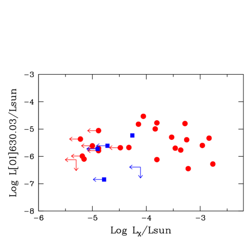
Figure 11: Luminosity of the [O i] 630.03 line plotted as a function of X-ray luminosity, when available, for the GTO sample. Red dots are the Lupus objects, blue filled squares are objects in $\sigma$ Ori. The X-ray luminosities were collected from the ROSAT observations by Krautter et al. (1997) for Lupus and from the XMM-Newton observations by Franciosini et al. (2006) for $\sigma$ Ori.

The difficulty of wind models to reproduce the LVC spectrum, and in particular the strength of the [O i] 557.79 line, pushed some authors to consider a different mechanism to excite the OI levels other than collisions with electrons and/or hydrogen atoms, namely photodissociation of OH in the disk surface layers (Störzer & Hollenbach, 2000; Acke et al., 2005; Rigliaco et al., 2013). The most detailed study of the LVC spectrum in a TTS has been carried on for TW Hya (M_star$\sim 0.7$ M_⊙, L_star$\sim 0.53$ L_⊙, $\dot{M}_{acc}$$\sim 10^{-9}$ M_⊙/yr) by Gorti et al. (2011) and Pascucci et al. (2011). TW Hya has a L([O i] 630.03)$\sim 1.110^{-5}$ L_⊙, a ratio [O i] 630.03/[O i] 557.79$\sim 7$, [S ii] 406.86/[O i] 630.03$\sim 0.13$, [S ii] 673.08/[S ii] 406.86$\mathbin{\lower 3.0pt\hbox{$\hbox to0.0pt{\raise 5.0pt\hbox{$\char 60\relax$}\hss}\mathchar 29208\relax$}}0.13$, not very different from the results we find in the GTO stars. Gorti et al. (2011) models that include X-ray and FUV photons fail to reproduce the [O i] 557.79 observed luminosity; this leads the authors to conclude that the strongest contribution to the two O i lines comes from photodissociation of OH, taking place on the disk surface, and O i lines do not trace a wind component. Only 20% of the [O i] 630.03 line is due to thermal processes in the dust-depleted inner disk, where also the [S ii] 406.86 line is emitted; the predicted global ratio [S ii] 406.86/[O i] 630.03$\sim 0.5$, is roughly consistent with the observations. Among TTS, TW Hya has rather unusual line profiles, with narrow lines (FWHM$\sim 10$ km/s) centered at zero velocity (Pascucci et al., 2011), which may support an origin in the disk surface, rather than in an unbound flow (but see Owen et al., 2010). Also, the presence of the dust-depleted inner ragion of radius $\sim 4$ AU seems crucial to the Gorti et al. (2011) model results.

The [S ii] 406.86 line provides the strongest discriminant between the two modes of line excitation, as it can only be produced by collisional excitation of S ii. As discussed in §6.3, in 65% of the GTO stars the luminosity of the three lines [O i] 630.03, [O i] 557.79 and [S ii] 406.86 is consistent with the emission expected in a high density, warm and neutral gas, where the lines are all thermally excited: a significant non-thermal contribution to the O i lines will reduce the [S ii] 406.86/[O i] 630.03 well below the observed values. We think that in these objects at least a non-thermal origin of the O i lines could be ruled out. There is, however, a small but not negligible fraction of objects (10 in total) with ratios [S ii] 406.86/[O i] 630.03 lower than predicted by thermal excitation, where models like that of TW Hya may apply. On the other hand, they do not seem to be in any way exceptional; they are distributed over the whole range of L_star, L_acc and L_X and the line profiles are similar to those of the other objects, broad with slightly blue-shifted peaks. Also, there is no evidence of an inner dust-depleted region similar to that in TW Hya but in a couple of cases (Rigliaco et al., 2012); Alcalá et al. in preparation).

An obvious caveat is in order, namely that the GTO spectra have relatively low spectral resolution; any detailed analysis and firm conclusion require higher quality data, to validate our assumption that all the lines are emitted by the same kinematical component. In view of its importance, it is interesting that in the past [S ii] 406.86 has not been searched for as extensively as the [O i] 630.03 line, even if one expects that their intensity should be similar.

7.3 Bound or Unbound gas?

The small velocity shift of the peak of the optical forbidden lines and their large width is difficult to understand in any wind model. Rigliaco et al. (2013) suggest that in two rather luminous TTS for which they have very high spectral resolution profiles of the [O i] 630.03 line, the LVC can be deconvolved into two different components, one narrower and slightly blueshifted, and one much broader and symmetric. The broad component, that contributes to $\sim$40% of the line intensity, does not trace unbound gas, but rather the emission coming from the inner region of the disk (a few tenth of AU), where the gas is gravitationally bound and in keplerian rotation around the star. The narrow component, on the other hand, could trace outflowing gas, ejected further out in the disk at the low velocity traced by the peak velocity shift.

This may be a general occurrence in TTS disks; Acke & van den Ancker (2006) propose a disk surface origin for the [O i] 630.03 line in HAe stars and in two cases convincingly derive the keplerian rotation and the disk orientation from high resolution $\Delta{\rm v}\sim 4$ km/s) spectra. We note that, if the Rigliaco et al. (2013) hypothesis is true for all objects, there should be an anticorrelation between the width of the broad, symmetric LVC component, which tends to zero if the disk is seen face-on, and the velocity of the HVC, which is maximum for face-on disk, as the jet is then expected to be oriented in the direction of the observer. A detailed study of high resolution profiles of the optical forbidden lines detected in the LVC of the GTO spectra, including the two [O i] 630.03, [O i] 557.79 and the [S ii] 406.86 lines, will be very valuable also from this point of view.

8 Summary and conclusions

We have examined in this paper the forbidden line spectrum of a sample of 44 low-mass TTS in the star forming regions Lupus and $\sigma$ Ori. The spectra have been obtained with X-Shooter, as part of the Italian GTO, and have been analyzed to derive stellar and accretion properties by Alcalá et al. (2014) and Rigliaco et al. (2012). All the GTO objects have a disk, as inferred from their IR excess emission, and are all accretors, with the exception of two stars in $\sigma$ Ori, where only upper limits to L_acc have been measured.

We detect forbidden lines of O i, O ii, S ii, N i and N ii in a number of stars. The line profiles show the presence of two components, one peaked close to zero velocity (LVC) and one with a large peak velocity shift (¿40 km/s) to the blue and/or to the red (HVC). The HVC has been identified with the emission of a high velocity jet, while the origin of the LVC is uncertain (Hartigan et al., 1995).

We focus our analysis on the LVC. The most commonly observed line is the [O i] 630.03, which is detected in 38/44 objects, followed by the other neutral oxygen line [O i] 557.79 and the [S ii] 406.86. In very few objects we have clear evidence of [S ii] 673.08 LVC emission. Higher excitation lines are detected with small peak velocity shifts in few objects, and probably trace a jet oriented along the plane of the sky. The spectral resolution of the GTO X-Shooter spectra ($\sim 30-60$ km/s) does not allow us to perform a detailed study of the gas kinematics. However, we can measure with reasonable accuracy the shift of the line peak, which is of few km/s to the blue for all the lines we have studied, and the line width, which is of $\sim 30-100$ km/s, with very few cases of unresolved lines. We confirm, for our low-mass sample, the properties of the LVC previously observed in solar-mass TTS; the small blue shift of the line peaks, in particular, seem to indicate their origin in outflowing, low velocity matter, which we call slow wind. We do not find any correlation between line profiles and stellar properties.

The GTO spectra show that slow winds are ubiquitous in Class II stars, i.e., in stars with circumstellar disks, independently of their stellar and/or accretion properties, down to the lowest mass stars in our sample (approximately 0.1 M_⊙, $\dot{M}_{acc}$$\sim 10^{-11}-10^{-12}$ M_⊙/yr. The slow wind, whose properties we derive from the analysis of the LVC of forbidden lines of O i and S ii, is prevalently neutral, dense ($n_{H}\mathbin{\lower 3.0pt\hbox{$\hbox to0.0pt{\raise 5.0pt\hbox{$\char 62\relax$}\hss}\mathchar 29208\relax$}}10^{8}$ cm^-3), warm (T$\sim 5000-10000$ K). These physical conditions do not seem to depend on the stellar and/or accretion properties. However, the mass of such gas varies by several orders of magnitude, from $\sim 10^{-12}$ M_⊙ for the lowest mass stars in our sample to $\sim 10^{-9}$ M_⊙ for solar-mass TTS. This may be accounted for by an increase in the density and/or the volume of the emitting matter.

We note that in about 65% of the objects the ratio of the [S ii] 406.86 to the [O i] 630.03 and [O i] 557.79 lines agrees with the predictions for a collisionally excited gas with the physical properties given above. This seems to rule out (at least in these objects) a non-thermal origin of the O i lines, as proposed by Hollenbach & Gorti (2009). However, in about 30% of cases, where we measure a relatively low [S ii] 406.86 intensity, this remains a viable hypothesis.

Line luminosities are strongly correlated with the stellar luminosity and with L_acc. In the latter case, the relation is not linear, but has a slope of $\sim 0.81\pm 0.09$. The results that the line luminosities correlate equally well with L_star and L_acc is not surprising, as these two quantities are themselves tightly correlated (L_acc $\propto$ L_star^1.53±0.18). As a consequence, we cannot establish which of these two properties drives the correlation with the line luminosity.

The comparison with the prediction of outflow models is difficult and, so far, the origin of the slow TTS winds remains elusive. In this context, the derivation of the mass and minimum volume of the low-velocity, dense and warm outflowing gas over a large range of stellar masses, luminosities and mass-accretion rates in §6.4 could provide crucial tests for wind models, even when calculations of the ionization and excitation conditions are not available.

On the observational side, we note that higher quality spectra, with higher spectral resolution and better sensitivity are necessary to confirm the results of our analysis and to derive the detailed kinematics and the origin of the line broadening (see, e.g., Rigliaco et al., 2013). Variability studies of the line profiles could also provide very valuable information on the ejection mechanisms.

Appendix A Stellar Properties

The stellar and accretion parameters for the GTO sample are listed in Table 3 (see Alcalá et al., 2014; Rigliaco et al., 2012).

Table 3: Stellar Properties

Name	$\alpha$(J2000)	$\delta$(J2000)	ST	T⋆	AV	L⋆	M⋆	Log Lacc	Log Macc	D
				(K)		(L⊙)	(M⊙)	(L⊙)	(M⊙/y)	(pc)
Sz66	15 39 28.28	-34 46 18.0	M3.0	3415	1.00	0.200	0.45	-1.8	-8.73	150
AKC2006-19	15 44 57.90	-34 23 39.5	M5.0	3125	0.00	0.016	0.10	-4.1	-10.85	150
Sz69	15 45 17.42	-34 18 28.5	M4.5	3197	0.00	0.088	0.20	-2.8	-9.50	150
Sz71	15 46 44.73	-34 30 35.5	M1.5	3632	0.50	0.309	0.62	-2.2	-9.23	150
Sz72	15 47 50.63	-35 28 35.4	M2.0	3560	0.75	0.252	0.45	-1.8	-8.73	150
Sz73	15 47 56.94	-35 14 34.8	K7	4060	3.50	0.419	1.00	-1.0	-8.26	150
Sz74	15 48 05.23	-35 15 52.8	M3.5	3342	1.50	1.043	0.50	-1.5	-8.09	150
Sz83	15 56 42.31	-37 49 15.5	K7	4060	0.00	1.313	1.15	-0.3	-7.37	150
Sz84	15 58 02.53	-37 36 02.7	M5.0	3125	0.00	0.122	0.17	-2.7	-9.24	150
Sz130	16 00 31.04	-41 43 37.2	M2.0	3560	0.00	0.160	0.45	-2.2	-9.23	150
Sz88A	16 07 00.54	-39 02 19.3	M0	3850	0.25	0.488	0.85	-1.2	-8.31	200
Sz88B	16 07 00.62	-39 02 18.1	M4.5	3197	0.00	0.118	0.20	-3.1	-9.74	200
Sz91	16 07 11.61	-39 03 47.1	M1	3705	1.20	0.311	0.62	-1.8	-8.85	200
Lup713	16 07 37.72	-39 21 38.8	M5.5	3057	0.00	0.020	0.08	-3.5	-10.08	200
Lup604s	16 08 00.20	-39 02 59.7	M5.5	3057	0.00	0.057	0.11	-3.7	-10.21	200
Sz97	16 08 21.79	-39 04 21.5	M4.0	3270	0.00	0.169	0.25	-2.9	-9.56	200
Sz99	16 08 24.04	-39 05 49.4	M4.0	3270	0.00	0.074	0.17	-2.6	-9.27	200
Sz100	16 08 25.76	-39 06 01.1	M5.5	3057	0.00	0.169	0.17	-3.0	-9.47	200
Sz103	16 08 30.26	-39 06 11.1	M4.0	3270	0.70	0.188	0.25	-2.4	-9.04	200
Sz104	16 08 30.81	-39 05 48.8	M5.0	3125	0.00	0.102	0.15	-3.2	-9.72	200
Lup706	16 08 37.30	-39 23 10.8	M7.5	2795	0.00	0.003	0.06	-4.8	-11.63	200
Sz106	16 08 39.76	-39 06 25.3	M0.5	3777	1.00	0.098	0.62	-2.5	-9.83	200
Par-Lup3-3	16 08 49.40	-39 05 39.3	M4.0	3270	2.20	0.239	0.25	-2.9	-9.49	200
Par-Lup3-4	16 08 51.43	-39 05 30.4	M4.5	3197	0.00	0.003	0.13	-4.1	-11.37	200
Sz110	16 08 51.57	-39 03 17.7	M4.0	3270	0.00	0.276	0.35	-2.0	-8.73	200
Sz111	16 08 54.69	-39 37 43.1	M1	3705	0.00	0.330	0.75	-2.2	-9.32	200
Sz112	16 08 55.52	-39 02 33.9	M5.0	3125	0.00	0.191	0.25	-3.2	-9.81	200
Sz113	16 08 57.80	-39 02 22.7	M4.5	3197	1.00	0.064	0.17	-2.1	-8.80	200
J160859	16 08 59.53	-38 56 27.6	M8.5	2600	0.00	0.009	0.03	-4.6	-10.80	200
c2dJ1609	16 09 01.40	-39 25 11.9	M4.0	3270	0.50	0.148	0.20	-3.0	-9.59	200
Sz114	16 09 01.85	-39 05 12.4	M4.8	3175	0.30	0.312	0.30	-2.5	-9.11	200
Sz115	16 09 06.21	-39 08 51.8	M4.5	3197	0.50	0.175	0.17	-2.7	-9.19	200
Lup818s	16 09 56.29	-38 59 51.7	M6.0	2990	0.00	0.025	0.08	-4.1	-10.63	200
Sz123A	16 10 51.34	-38 53 14.6	M1	3705	1.25	0.203	0.60	-1.8	-8.93	200
Sz123B	16 10 51.31	-38 53 12.8	M2.0	3560	0.00	0.051	0.50	-2.7	-10.03	200
SST-Lup3-1	16 11 59.81	-38 23 38.5	M5.0	3125	0.00	0.059	0.13	-3.6	-10.17	200
SO397	05 38 13.18	-02 26 08.6	M4.5	3200	0.00	0.19	0.20	-2.71	-9.42	360
SO490	05 38 23.58	-02 20 47.5	M5.5	3060	0.00	0.08	0.14	-3.10	-9.97	360
SO500	05 38 25.41	-02 42 41.2	M6	2990	0.00	0.02	0.08	-3.95	-10.27	360
SO587	05 38 34.04	-02 36 37.3	M4.5	3200	0.00	0.28	0.20	$<$-4	$<$-10.41	360
SO646	05 38 39.01	-02 45 32.0	M3.5	3350	0.00	0.10	0.30	-3.00	-9.68	360
SO848	05 39 01.94	-02 35 02.8	M4	3270	0.00	0.02	0.19	-3.50	-10.39	360
SO1260	05 39 53.63	-02 33 42.9	M4	3270	0.00	0.13	0.26	-2.00	-8.97	360
SO1266	05 39 54.22	-02 27 32.9	M4.5	3200	0.00	0.06	0.20	$<$-4.85	$<$-11.38	360

Appendix B Line properties

Tables LABEL:tab_tabellone_1, LABEL:tab_tabellone_2, LABEL:tab_tabellone_3 and LABEL:tab_tabellone_4 list the properties of the LVC, HVC-blue shifted and HVC-red shifted components of the lines [O i] 557.79, [O i] 630.03, [O ii] 372.60, [O ii] 731.89, [S ii] 406.86, [S ii] 673.08, and [N ii] 658.34. For each component the tables give the intensity, the uncertainty, the velocity shift of the line peak and the FWHM of the observed component. When not detected, we give $3\sigma$ upper limit for the LVC only.

Table 4: Fluxes, velocity peak and full-width half maximun of [O i] lines

name

[O i] 557.79

[O i] 630.03

LVC

LVC

HVC-Blue

HVC-Red

flux

Vpeak

FWHM

flux

Vpeak

FWHM

flux

Vpeak

FWHM

flux

Vpeak

FWHM

(erg s-1 cm-2)

(km s-1)

(km s-1)

(erg s-1 cm-2)

(km s-1)

(km s-1)

(erg s-1 cm-2)

(km s-1)

(km s-1)

(erg s-1 cm-2)

(km s-1)

(km s-1)

Sz66

3.68($\pm$0.20)e-15

-13.2

72.4

2.25($\pm$0.06)e-14

-19.4

48.6

…

…

…

…

…

…

AKC2006-1

$<$1.50e-17

…

…

$<$2.85e-17

…

…

…

…

…

…

…

…

Sz69

2.08($\pm$0.16)e-15

-10.9

59†

6.09($\pm$0.20)e-15

-7.7

55.5

3.44($\pm$0.10)e-15

-92.9

73.5

1.34($\pm$0.50)e-15

58.8

48.3

Sz71

2.60($\pm$0.50)e-15

-13.9

68.3

3.00($\pm$0.10)e-15

-1

97.5

…

…

…

…

…

…

Sz72

1.80($\pm$0.60)e-15

-15.2

72.1

2.80($\pm$0.40)e-15

-10.8

42.2

4.57($\pm$0.70)e-15

-125.0

72.3

…

…

…

Sz73

7.10($\pm$0.25)e-15

-27.5

59†

4.15($\pm$0.02)e-14

-18.9

60.8

9.32($\pm$0.04)e-14

-94.2

59.1

…

…

…

Sz74

1.25($\pm$0.30)e-14

7.3

76.5

2.13($\pm$0.25)e-14

-7.5

40.5

…

…

…

…

…

…

Sz83

…

…

…

…

…

…

…

…

…

…

…

…

Sz84

3.20($\pm$0.80)e-16

-8.4

76.7

1.45($\pm$0.15)e-15

-7.4

41.4

…

…

…

…

…

…

Sz130

1.33($\pm$0.18)e-15

-8.1

74.9

2.14($\pm$0.30)e-15

17.7

72.9

4.79($\pm$0.60)e-15

-49.3

57.4

…

…

…

Sz88A

6.07($\pm$0.30)e-15

-1.9

62.7

1.34($\pm$0.10)e-14

-1.7

53.5

…

…

…

…

…

…

Sz88B

2.04($\pm$0.40)e-16

-7.1

67.9

6.07($\pm$0.80)e-16

-3.9

55.6

…

…

…

…

…

…

Sz91

1.65($\pm$0.30)e-15

-2.3

70.2

4.00($\pm$0.48)e-15

-3.4

34†

…

…

…

…

…

…

Lup713

$<$8.00e-17

…

…

$<$4.30e-17

4.2

34†

…

…

…

…

…

…

Lup604s

$<$1.60e-16

…

…

1.58($\pm$0.16)e-16

-2.5

50.1

…

…

…

…

…

…

Sz97

$<$2.50e-16

…

…

2.83($\pm$0.80)e-16

-36.4

58.4

…

…

…

…

…

…

Sz99

8.60($\pm$0.80)e-16

-10.0

92.0

1.36($\pm$0.09)e-15

3.3

77.2

…

…

…

2.20($\pm$0.60)e-16

72.8

51.0

Sz100

9.01($\pm$0.90)e-16

-16.0

73.6

3.24($\pm$0.20)e-15

-6.6

43.7

3.98($\pm$0.20)e-15

-54.6

84.6

4.06($\pm$1.30)e-16

56.2

50.2

Sz103

6.24($\pm$0.90)e-16

-9.0

73.3

3.70($\pm$0.30)e-15

-32.4

54.9

…

…

…

…

…

…

Sz104

1.74($\pm$0.50)e-16

-6.0

59†

4.18($\pm$0.50)e-16

-6.8

40.1

…

…

…

…

…

…

Lup706

$<$6.50e-17

…

…

$<$1.74e-17

…

…

…

…

…

…

…

…

Sz106

4.14($\pm$0.50)e-16

-14.5

70.2

2.00($\pm$0.20)e-15

-9.6

108.1

…

…

…

…

…

…

Par-Lup3-3

$<$3.00e-15

…

…

3.41($\pm$0.50)e-15

-1.4

64.8

…

…

…

…

…

…

Par-Lup3-4

2.38($\pm$0.22)e-16

-4.6

78.2

4.69($\pm$0.50)e-15

0.6

65.6

…

…

…

…

…

…

Sz110

1.40($\pm$0.28)e-15

4.9

98.3

1.65($\pm$0.25)e-15

-7.1

66.7

…

…

…

…

…

…

Sz111

2.20($\pm$0.60)e-15

0.6

63.6

8.06($\pm$0.80)e-15

-2.9

46.8

…

…

…

…

…

…

Sz112

7.19($\pm$1.00)e-16

0.2

68.2

1.94($\pm$0.15)e-15

-2.4

49.6

…

…

…

…

…

…

Sz113

3.00($\pm$1.00)e-16

-10.0

66.0

6.37($\pm$0.60)e-16

-12.3

34†

2.17($\pm$0.15)e-15

-122.6

54.6

…

…

…

J160859

4.57($\pm$1.00)e-17

-40.6

59†

2.69($\pm$0.30)e-16

-16.8

58.3

…

…

…

…

…

…

c2dJ1609

7.75($\pm$1.00)e-16

-9.1

81.2

3.18($\pm$0.40)e-15

-9.9

74.8

…

…

…

…

…

…

Sz114

8.95($\pm$1.50)e-16

0.5

48.2

1.59($\pm$0.20)e-15

-10.1

43.9

1.32($\pm$0.20)e-15

-93.3

77.3

…

…

…

Sz115

$<$7.00e-16

…

…

$<$6.00e-16

…

…

…

…

…

…

…

…

Lup818s

5.00($\pm$1.70)e-17

-40.0

59†

1.30($\pm$0.17)e-16

-7.2

43.3

…

…

…

…

…

…

Sz123A

2.63($\pm$0.80)e-15

-14.4

81.6

6.96($\pm$0.40)e-15

-10.1

64.8

2.39($\pm$0.15)e-15

-61.9

61.4

…

…

…

Sz123B

4.46($\pm$0.40)e-16

-6.8

78.2

1.29($\pm$0.08)e-15

-10.6

66.2

4.15($\pm$1.00)e-16

-69.6

65.8

…

…

…

SST-Lup3-1

$<$1.40e-16

…

…

$<$1.00e-16

…

…

…

…

…

…

…

…

SO397

$<$4.00e-17

…

…

$<$1.00e-16

…

…

…

…

…

…

…

…

SO490

3.30($\pm$0.40)e-17

-21.0

61.9

5.15($\pm$1.00)e-17

-22.7

62.8

…

…

…

…

…

…

SO500

$<$2.00e-17

…

…

2.40($\pm$0.70)e-17

-21.2

80.9

3.53($\pm$1.00)e-18

-70.3

16.8

…

…

…

SO587

$<$1.70e-16

…

…

1.43($\pm$0.07)e-15

-7.5

56.0

…

…

…

…

…

…

SO646

$<$6.40e-17

…

…

6.00($\pm$0.60)e-16

-9.3

71.8

…

…

…

…

…

…

SO848

6.30($\pm$0.40)e-17

-2.5

63.9

4.61($\pm$0.15)e-16

-8.5

42.2

3.60($\pm$0.10)e-16

-51.8

48.6

…

…

…

SO1260

2.60($\pm$0.30)e-16

-5.8

59†

4.20($\pm$0.35)e-16

-6.6

41.7

…

…

…

…

…

…

SO1266

2.80($\pm$1.00)e-17

-9.1

59†

1.88($\pm$0.20)e-16

-7.5

49.2

…

…

…

…

…

…

• ^† : Not resolved line; the FWHM is the instrumental resolution (e.g., 59 km/s for the [O i] 557.79 line and 34 km/s for the [O i] 630.03 line).

Table 5: Fluxes, velocity peak and full-width half maximun of [O ii] lines

name

[O ii] 372.60

[O ii] 731.89

LVC

HVC-Blue

HVC-Red

LVC

HVC-Blue

HVC-Red

flux

Vpeak

FWHM

flux

Vpeak

FWHM

flux

Vpeak

FWHM

flux

Vpeak

FWHM

flux

Vpeak

FWHM

flux

Vpeak

FWHM

(erg s-1 cm-2)

(km s-1)

(km s-1)

(erg s-1 cm-2)

(km s-1)

(km s-1)

(erg s-1 cm-2)

(km s-1)

(km s-1)

(erg s-1 cm-2)

(km s-1)

(km s-1)

(erg s-1 cm-2)

(km s-1)

(km s-1)

(erg s-1 cm-2)

(km s-1)

(km s-1)

Sz66

4.27($\pm$1.00)e-16

-36.4

62.8

…

…

…

…

…

…

$<$1.91e-15

…

…

…

…

…

…

…

…

AKC2006-1

$<$1.50e-17

…

…

…

…

…

…

…

…

$<$9.42e-17

…

…

…

…

…

…

…

…

Sz69

$<$2.00e-16

…

…

…

…

…

4.30($\pm$1.20)e-16

107.5

76.6

$<$2.08e-16

…

…

…

…

…

…

…

…

Sz71

$<$1.90e-16

…

…

…

…

…

…

…

…

$<$1.91e-15

…

…

…

…

…

…

…

…

Sz72

$<$1.50e-15

…

…

…

…

…

4.20($\pm$0.50)e-15

101.7

86.4

$<$1.70e-15

…

…

…

…

…

…

…

…

Sz73

$<$4.00e-15

…

…

6.00($\pm$1.80)e-15

-96.1

76.9

…

…

…

3.00($\pm$0.50)e-15

-10.0

45.0

7.6($\pm$0.50)e-15

-109.0

37.0

…

…

…

Sz74

$<$1.60e-15

…

…

…

…

…

…

…

…

$<$6.00e-15

…

…

…

…

…

…

…

…

Sz83

…

…

…

…

…

…

…

…

…

…

…

…

…

…

…

…

…

…

Sz84

7.69($\pm$2.5)e-17

-16.8

59†

…

…

…

…

…

…

$<$7.72e-16

…

…

…

…

…

…

…

…

Sz130

$<$6.00e-16

…

…

…

…

…

…

…

…

$<$8.33e-16

…

…

…

…

…

…

…

…

Sz88A

$<$3.70e-15

…

…

…

…

…

…

…

…

$<$1.00e-15

…

…

…

…

…

…

…

…

Sz88B

$<$4.00e-17

…

…

…

…

…

…

…

…

$<$5.08e-16

…

…

…

…

…

…

…

…

Sz91

$<$1.70e-16

…

…

…

…

…

…

…

…

$<$1.61e-15

…

…

…

…

…

…

…

…

Lup713

$<$1.60e-17

…

…

…

…

…

…

…

…

$<$4.01e-17

…

…

…

…

…

…

…

…

Lup604s

$<$3.10e-17

…

…

…

…

…

…

…

…

$<$1.29e-16

…

…

…

…

…

…

…

…

Sz97

$<$1.00e-16

…

…

…

…

…

…

…

…

$<$4.17e-16

…

…

…

…

…

…

…

…

Sz99

…

…

…

…

…

…

3.12($\pm$0.50)e-16

83.1

73.5

$<$1.61e-16

…

…

…

…

…

…

…

…

Sz100

…

…

…

2.99($\pm$0.70)e-16

-64.0

59†

…

…

…

$<$5.29e-16

…

…

…

…

…

…

…

…

Sz103

$<$1.50e-16

…

…

…

…

…

…

…

…

$<$6.65e-16

…

…

…

…

…

…

…

…

Sz104

$<$4.80e-17

…

…

…

…

…

…

…

…

$<$4.01e-16

…

…

…

…

…

…

…

…

Lup706

$<$1.00e-17

…

…

…

…

…

…

…

…

$<$1.19e-17

…

…

…

…

…

…

…

…

Sz106

4.96($\pm$0.30)e-16

-0.9

120.0

…

…

…

…

…

…

$<$2.28e-16

…

…

…

…

…

…

…

…

Par-Lup3-3

$<$6.00e-16

…

…

…

…

…

…

…

…

$<$6.25e-16

…

…

…

…

…

…

…

…

Par-Lup3-4

3.01($\pm$1.00)e-17

28.0

92.4

…

…

…

…

…

…

5.00($\pm$1.30)e-17

0.0

69.0

…

…

…

…

…

…

Sz110

$<$3.50e-16

…

…

…

…

…

…

…

…

$<$1.09e-15

…

…

…

…

…

…

…

…

Sz111

$<$1.20e-16

…

…

…

…

…

…

…

…

$<$1.33e-15

…

…

…

…

…

…

…

…

Sz112

$<$5.30e-17

…

…

…

…

…

…

…

…

$<$1.19e-15

…

…

…

…

…

…

…

…

Sz113

$<$4.00e-15

…

…

…

…

…

…

…

…

$<$2.26e-16

…

…

…

…

…

…

…

…

J160859

$<$2.00e-17

…

…

…

…

…

…

…

…

$<$2.45e-17

…

…

…

…

…

…

…

…

c2dJ1609

$<$2.00e-16

…

…

…

…

…

…

…

…

$<$6.25e-16

…

…

…

…

…

…

…

…

Sz114

$<$1.10e-16

…

…

…

…

…

…

…

…

$<$1.75e-15

…

…

…

…

…

…

…

…

Sz115

$<$1.00e-16

…

…

…

…

…

…

…

…

$<$5.94e-16

…

…

…

…

…

…

…

…

Lup818s

$<$3.30e-17

…

…

…

…

…

…

…

…

$<$7.57e-17

…

…

…

…

…

…

…

…

Sz123A

$<$1.20e-15

…

…

…

…

…

…

…

…

$<$1.32e-15

…

…

…

…

…

…

…

…

Sz123B

$<$1.20e-16

…

…

…

…

…

…

…

…

$<$3.36e-16

…

…

…

…

…

…

…

…

SST-Lup3-1

$<$3.00e-17

…

…

…

…

…

…

…

…

$<$2.62e-16

…

…

…

…

…

…

…

…

SO397

$<$1.60e-17

…

…

…

…

…

…

…

…

$<$1.90e-16

…

…

…

…

…

…

…

…

SO490

$<$9.10e-18

…

…

…

…

…

…

…

…

$<$6.35e-17

…

…

…

…

…

…

…

…

SO500

$<$1.00e-17

…

…

…

…

…

…

…

…

$<$1.04e-17

…

…

…

…

…

…

…

…

SO587

2.43($\pm$0.04)e-15

-6.5

63.3

…

…

…

…

…

…

$<$1.39e-16

…

…

…

…

…

…

…

…

SO646

$<$2.40e-17

…

…

…

…

…

…

…

…

$<$1.15e-16

…

…

…

…

…

…

…

…

SO848

$<$1.50e-16

…

…

9.42($\pm$0.50)e-16

-40.4

79.0

…

…

…

1.60($\pm$0.18)e-16

-26.0

69.0

…

…

…

…

…

…

SO1260

…

…

…

…

…

…

…

…

…

$<$1.86e-16

…

…

…

…

…

…

…

…

SO1266

…

…

…

1.04($\pm$0.24)e-16

-64.0

59†

…

…

…

$<$9.67e-17

…

…

…

…

…

…

…

…

• ^† : Not resolved line; the FWHM is the instrumental resolution (e.g., 59 km/s for the [O ii] 372.60 line and 34 km/s for the [O ii] 731.89 line).

Table 6: Fluxes, velocity peak and full-width half maximun of [S ii] lines

name

[S ii] 406.86

[S ii] 673.08

LVC

HVC-Blue

HVC-Red

LVC

HVC-Blue

HVC-Red

flux

Vpeak

FWHM

flux

Vpeak

FWHM

flux

Vpeak

FWHM

flux

Vpeak

FWHM

flux

Vpeak

FWHM

flux

Vpeak

FWHM

(erg s-1 cm-2)

(km s-1)

(km s-1)

(erg s-1 cm-2)

(km s-1)

(km s-1)

(erg s-1 cm-2)

(km s-1)

(km s-1)

(erg s-1 cm-2)

(km s-1)

(km s-1)

(erg s-1 cm-2)

(km s-1)

(km s-1)

(erg s-1 cm-2)

(km s-1)

(km s-1)

Sz66

5.63($\pm$0.40)e-15

-22.7

60.0

…

…

…

…

…

…

6.89($\pm$2.00)e-16

-19.5

38.2

…

…

…

…

…

…

AKC2006-1

$<$2.00e-17

…

…

…

…

…

…

…

…

$<$2.30e-17

…

…

…

…

…

…

…

…

Sz69

1.27($\pm$0.15)e-15

-8.4

81.0

6.80($\pm$0.80)e-16

-99.6

67.5

5.50(2.00)e-17

80.1

22.0

$<$4.60e-16

…

…

2.69($\pm$0.50)e-16

-103.2

51.6

3.88($\pm$0.70)e-16

62.2

37.5

Sz71

$<$2.10e-15

…

…

…

…

…

…

…

…

$<$1.40e-15

…

…

…

…

…

…

…

…

Sz72

$<$3.00e-15

…

…

3.20($\pm$1.00)e-15

-133.2

117.7

…

…

…

$<$5.00e-16

…

…

1.50($\pm$0.30)e-15

-132.2

40.8

…

…

…

Sz73

$<$1.00e-14

…

…

2.60($\pm$0.40)e-14

-96.3

79.8

…

…

…

$<$1.00e-15

…

…

8.40($\pm$2.00)e-15

-98.3

64.9

…

…

…

Sz74

3.00($\pm$0.60)e-15

-15.8

59†

…

…

…

…

…

…

$<$3.00e-15

…

…

…

…

…

…

…

…

Sz83

…

…

…

…

…

…

…

…

…

…

…

…

…

…

…

…

…

…

Sz84

$<$1.30e-16

…

…

…

…

…

…

…

…

$<$1.90e-16

…

…

…

…

…

…

…

…

Sz130

$<$6.00e-16

…

…

6.40($\pm$2.00)e-16

-49.9

73.8

…

…

…

$<$5.90e-16

…

…

…

…

…

…

…

…

Sz88A

3.63($\pm$0.30)e-15

3.8

65.6

…

…

…

…

…

…

$<$4.70e-16

…

…

…

…

…

…

…

…

Sz88B

1.02($\pm$0.20)e-16

-4.2

65.5

…

…

…

…

…

…

$<$1.40e-16

…

…

…

…

…

…

…

…

Sz91

$<$1.00e-15

…

…

…

…

…

…

…

…

$<$1.00e-15

…

…

…

…

…

…

…

…

Lup713

$<$1.50e-17

…

…

…

…

…

…

…

…

$<$1.50e-17

…

…

…

…

…

…

…

…

Lup604s

$<$5.80e-17

…

…

…

…

…

…

…

…

$<$5.00e-17

…

…

…

…

…

…

…

…

Sz97

$<$9.90e-17

…

…

…

…

…

…

…

…

$<$2.40e-16

…

…

…

…

…

…

…

…

Sz99

4.74($\pm$1.00)e-16

-4.4

84.2

…

…

…

9.23(3.00)e-17

87.0

48.7

$<$1.00e-16

…

…

…

…

…

2.17($\pm$0.70)e-16

61.9

80.7

Sz100

1.46($\pm$0.15)e-15

-23.4

68.0

4.30($\pm$1.00)e-16

-90.7

69.1

…

…

…

4.68($\pm$1.20)e-16

-12.3

52.3

4.66($\pm$1.20)e-16

-71.2

61.8

…

…

…

Sz103

1.38($\pm$1.80)e-15

-29.8

63.9

…

…

…

…

…

…

2.20($\pm$0.70)e-16

-37.5

34†

…

…

…

…

…

…

Sz104

3.63($\pm$0.80)e-16

-1.6

58

…

…

…

…

…

…

$<$1.00e-16

…

…

…

…

…

…

…

…

Lup706

$<$1.00e-17

…

…

…

…

…

…

…

…

$<$7.90e-18

…

…

…

…

…

…

…

…

Sz106

2.98($\pm$0.18)e-15

-34.4

136.4

…

…

…

…

…

…

5.68($\pm$1.00)e-16

0.5

80.1

…

…

…

…

…

…

Par-Lup3-3

$<$8.16e-16

…

…

…

…

…

…

…

…

$<$4.10e-16

…

…

…

…

…

…

…

…

Par-Lup3-4

1.73($\pm$0.04)e-15

3.9

76.4

…

…

…

…

…

…

1.27($\pm$0.02)e-15

10.3

70.1

…

…

…

…

…

…

Sz110

1.48($\pm$0.30)e-15

-25.7

118.4

…

…

…

…

…

…

$<$2.00e-16

…

…

…

…

…

…

…

…

Sz111

$<$6.00e-16

…

…

…

…

…

…

…

…

$<$5.80e-16

…

…

…

…

…

…

…

…

Sz112

2.40($\pm$0.60)e-16

-4.0

58

…

…

…

…

…

…

$<$1.40e-16

…

…

…

…

…

…

…

…

Sz113

$<$4.00e-16

…

…

2.33($\pm$0.50)e-15

-124.6

73.71

…

…

…

$<$1.00e-16

…

…

7.60($\pm$0.50)e-16

-120.9

65.5

…

…

…

J160859

7.98($\pm$1.70)e-17

-38.4

69.0

…

…

…

…

…

…

…

…

…

…

…

…

…

…

…

c2dJ1609

7.94($\pm$1.50)e-16

-12.5

95.1

…

…

…

…

…

…

$<$3.50e-16

…

…

…

…

…

…

…

…

Sz114

5.39($\pm$1.30)e-16

-1.6

59.9

…

…

…

…

…

…

$<$5.40e-16

…

…

…

…

…

…

…

…

Sz115

$<$6.40e-17

…

…

…

…

…

…

…

…

$<$1.90e-16

…

…

…

…

…

…

…

…

Lup818s

$<$3.50e-17

…

…

…

…

…

…

…

…

$<$1.80e-17

…

…

…

…

…

…

…

…

Sz123A

2.10($\pm$0.40)e-15

-21.7

89.7

5.80($\pm$1.00)e-16

-103.3

65.6

…

…

…

$<$4.00e-16

…

…

…

…

…

…

…

…

Sz123B

1.70($\pm$0.25)e-16

7.4

76.3

1.00($\pm$0.50)e-16

-65.5

58.0

…

…

…

$<$9.00e-17

…

…

…

…

…

…

…

…

SST-Lup3-1

$<$3.50e-17

…

…

…

…

…

…

…

…

$<$6.00e-17

…

…

…

…

…

…

…

…

SO397

$<$1.70e-17

…

…

…

…

…

…

…

…

$<$8.00e-17

…

…

…

…

…

…

…

…

SO490

$<$1.40e-17

…

…

…

…

…

…

…

…

$<$1.60e-17

…

…

…

…

…

…

…

…

SO500

$<$3.00e-18

…

…

…

…

…

…

…

…

$<$4.00e-18

…

…

…

…

…

…

…

…

SO587

7.58($\pm$0.70)e-16

-8.0

74.6

…

…

…

…

…

…

2.14($\pm$0.02)e-15

-9.1

48.1

…

…

…

…

…

…

SO646

9.11($\pm$2.00)e-17

-26.7

90.3

…

…

…

…

…

…

$<$8.00e-17

…

…

…

…

…

…

…

…

SO848

$<$5.00e-17

…

…

3.47($\pm$0.17)e-16

-46.9

75.6

…

…

…

3.26($\pm$0.25)e-16

-3.0

50.0

4.48($\pm$0.25)e-16

-47.3

49.6

…

…

…

SO1260

1.14($\pm$0.20)e-16

-27.2

61.0

…

…

…

…

…

…

$<$4.00e-17

…

…

…

…

…

…

…

…

SO1266

$<$3.00e-17

…

…

2.80($\pm$1.00)e-17

-68.4

59†

…

…

…

4.71($\pm$1.50)e-17

-4.1

34†

…

…

…

…

…

…

• ^† : Not resolved line; the FWHM is the instrumental resolution (e.g., 59 km/s for the [S ii] 406.86 line and 34 km/s for the [S ii] 673.08 line).

Table 7: Fluxes, velocity peak and full-width half maximun of [N ii] lines

name	[N ii] 658.34
	LVC			HVC-Blue			HVC-Red
	flux	Vpeak	FWHM	flux	Vpeak	FWHM	flux	Vpeak	FWHM
	(erg s-1 cm-2)	(km s-1)	(km s-1)	(erg s-1 cm-2)	(km s-1)	(km s-1)	(erg s-1 cm-2)	(km s-1)	(km s-1)
Sz66	1.12($\pm$0.30)e-15	-36.7	37.9	…	…	…	…	…	…
AKC2006-1	$<$5.0e-17	…	…	…	…	…	…	…	…
Sz69	…	…	…	3.12($\pm$1.00)e-16	-90.3	62.7	1.72($\pm$0.50)e-16	57.0	44.3
Sz71	$<$8.00e-16	…	…	…	…	…	…	…	…
Sz72	$<$8.00e-16	…	…	…	…	…	…	…	…
Sz73	$<$8.00e-15	…	…	1.60($\pm$0.30)e-14	-94.5	103.0	…	…	…
Sz74	$<$3.00e-15	…	…	…	…	…	…	…	…
Sz83	$<$3.60e-15	…	…	…	…	…	…	…	…
Sz84	…	…	…	…	…	…	…	…	…
Sz130	$<$7.50e-16	…	…	1.00($\pm$0.26)e-15	-56.5	40.8	…	…	…
Sz88A	$<$5.00e-16	…	…	…	…	…	…	…	…
Sz88B	$<$2.30e-16	…	…	…	…	…	…	…	…
Sz91	$<$6.40e-16	…	…	…	…	…	…	…	…
Lup713	$<$1.50e-17	…	…	…	…	…	…	…	…
Lup604s	$<$9.00e-17	…	…	…	…	…	…	…	…
Sz97	$<$3.60e-16	…	…	…	…	…	…	…	…
Sz99	$<$6.70e-17	…	…	…	…	…	…	…	…
Sz100	…	…	…	4.82($\pm$1.00)e-16	-70.8	34.9	…	…	…
Sz103	…	…	…	5.37($\pm$1.00)e-16	-40.2	34†	…	…	…
Sz104	$<$2.00e-16	…	…	…	…	…	…	…	…
Lup706	$<$7.60e-18	…	…	…	…	…	…	…	…
Sz106	4.50($\pm$1.00)e-16	-1.0	85.0	…	…	…	…	…	…
Par-Lup3-3	$<$3.00e-16	…	…	…	…	…	…	…	…
Par-Lup3-4	2.22($\pm$0.25)e-16	10.2	70.0	…	…	…	…	…	…
Sz110	$<$4.00e-16	…	…	…	…	…	…	…	…
Sz111	$<$6.50e-16	…	…	…	…	…	…	…	…
Sz112	$<$3.20e-16	…	…	…	…	…	…	…	…
Sz113	…	…	…	1.29($\pm$4.00)e-16	-125.1	40.6	…	…	…
J160859	$<$2.00e-17	…	…	…	…	…	…	…	…
c2dJ1609	6.89($\pm$1.00)e-16	-33.4	46.2	…	…	…	…	…	…
Sz114	$<$6.70e-16	…	…	…	…	…	…	…	…
Sz115	$<$3.30e-16	…	…	…	…	…	…	…	…
Lup818s	$<$4.50e-17	…	…	…	…	…	…	…	…
Sz123A	…	…	…	9.27($\pm$3.00)e-16	-55.8	38.9	…	…	…
Sz123B	…	…	…	2.00($\pm$0.40)e-16	-56.6	44.4	…	…	…
SST-Lup3-1	$<$1.00e-16	…	…	…	…	…	…	…	…
SO397	$<$1.30e-16	…	…	…	…	…	…	…	…
SO490	$<$2.80e-17	…	…	…	…	…	…	…	…
SO500	$<$7.30e-18	…	…	…	…	…	…	…	…
SO587	4.35($\pm$0.25)e-15	-8.9	45.2	…	…	…	…	…	…
SO646	$<$9.40e-17	…	…	…	…	…	…	…	…
SO848	1.67($\pm$0.05)e-15	-0.5	37.8	6.01($\pm$0.50)e-16	-47.9	50.7	…	…	…
SO1260	$<$9.20e-17	…	…	…	…	…	…	…	…
SO1266	$<$6.3	…	…	…	…	…	…	…	…

Notes:

• ^† : Not resolved line; the FWHM is the instrumental resolution (e.g., 34 km/s for the [N ii] 658.34 line).

Appendix C Examples of line profiles in selected objects

In this Appendix we show examples of the line profiles discussed in this paper.

Figure 12: Normalized, continuum subtracted line profile of the [O i] 630.03 line. The profiles are shifted vertically for an easier display.

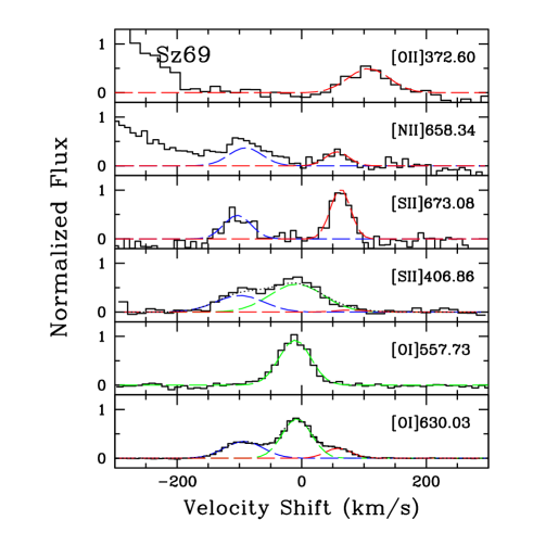
Figure 14: Same as Fig. 13 for Sz69.

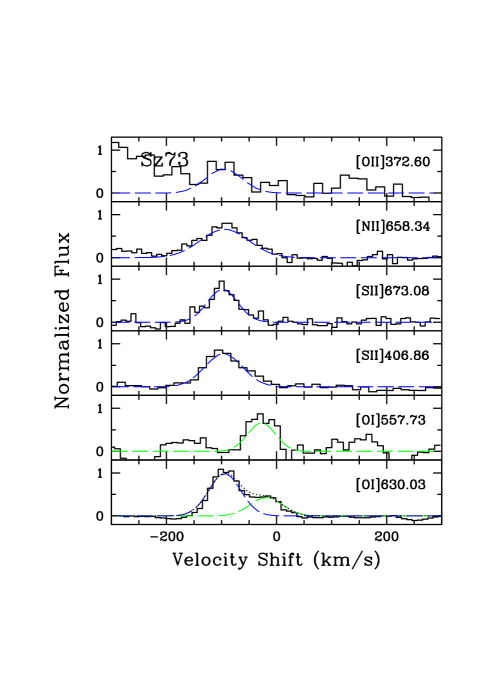
Figure 15: Same as Fig. 13 for Sz73.

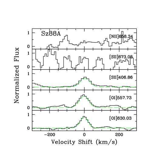
Figure 16: Same as Fig. 13 for Sz88A. The two panels for the lines [N ii] 658.34 and [S ii] 673.08 illustrate typical non-detections.

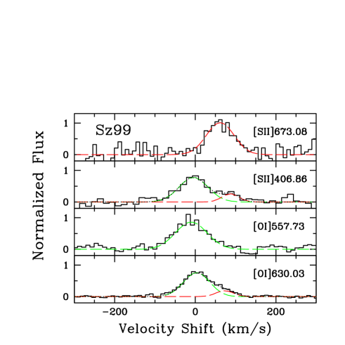
Figure 17: Same as Fig. 13 for Sz99.

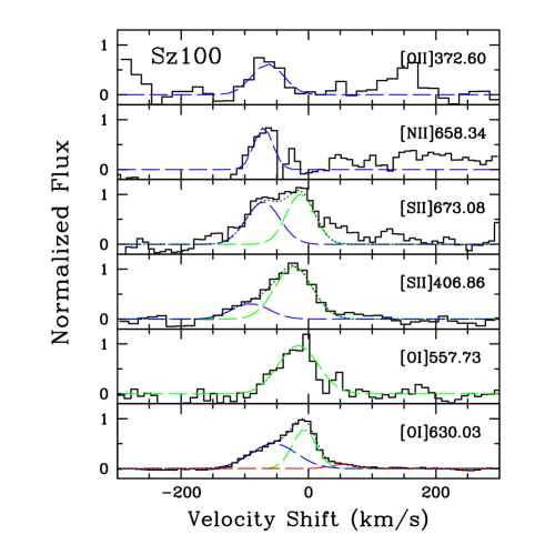
Figure 18: Same as Fig. 13 for Sz100.

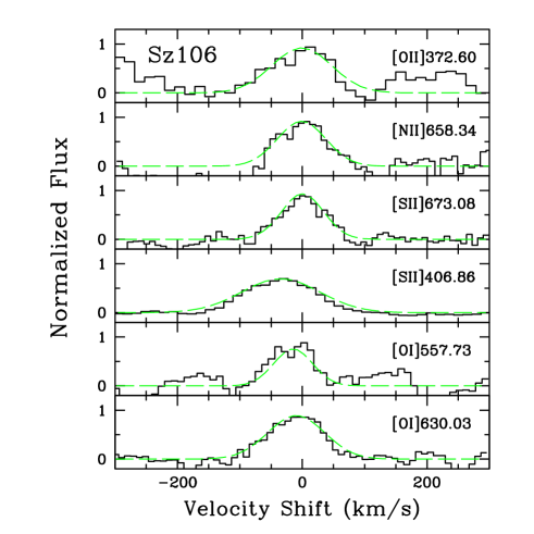
Figure 19: Same as Fig. 13 for Sz106.

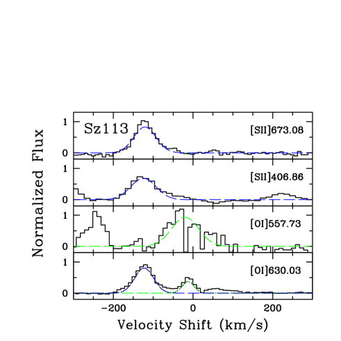
Figure 20: Same as Fig. 13 for Sz113. Note that the [O i] 557.79 is a 3$\sigma$ detection.

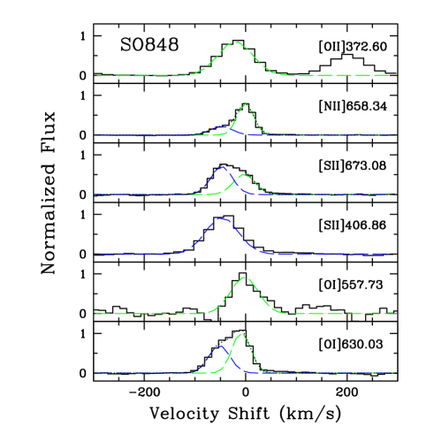
Figure 21: Same as Fig. 13 for SO848.