Excluded-Volume Approximation for Supernova Matter

Abstract

A general scheme of the excluded-volume approximation as applied to multicomponent systems with an arbitrary degree of degeneracy has been developed. This scheme also admits an allowance for additional interactions between the components of a system. A specific form of the excluded-volume approximation for investigating supernova matter at subnuclear densities has been found from comparison with the hard-sphere model. The possibility of describing the phase transition to uniform nuclear matter in terms of the formalism under consideration is discussed.

Institute for Theoretical and Experimental Physics, ul. Bol’shaya Cheremushkinskaya 25, Moscow, 117259 Russia

Keywords:

nuclear astrophysics, stars—structure and evolution.

INTRODUCTION

The evolution of massive stars ends with the formation of a central ‘‘iron’’ core. This core loses its hydrodynamic stability and is drawn into gravitational collapse that eventually leads to a supernova explosion. In the course of collapse, the density in the central regions of the star rises to values comparable to the density of matter inside atomic nuclei, $\rho_{\mathrm{n}}\simeq 2.6\times 10^{14}\ \mbox{g\,cm${}^{-3}$}$. Under these conditions, when the mean distances between atomic nuclei are comparable to their sizes, a strong nuclear interaction confining the nucleons inside the nucleus begins to manifest itself. Nuclei with a mass number up to $A\sim 100$ begin to fuse, stretch, and deform. As a result, peculiar configurations known as ‘‘lasagna’’, ‘‘pasta’’, etc. are formed. At a density $\rho\sim 0.5\rho_{\mathrm{n}}$ the phase transition to uniform nuclear matter occurs.

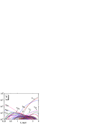
Figure 1: (Color online) Chemical composition of matter at $\rho=10^{13}\leavevmode\nobreak\ \mbox{g\,cm${}^{-3}$}$ and $\mbox{$Y_{\mathrm{e}}$}=26/56$

Figure 1 shows an example of the calculation of equilibrium mass fractions for matter $\mbox{$Y_{\mathrm{i}}$}\equiv n_{i}\mbox{$m_{\mathrm{u}}$}/\rho$, where $n_{i}$ — is the number density of component $i$, as a function of the temperature at density $\rho=10^{13}\leavevmode\nobreak\ \mbox{g\,cm${}^{-3}$}$ and leptonic number $\mbox{$Y_{\mathrm{e}}$}=26/56$. The calculation was performed by assuming the nuclear statistical equilibrium (NSE, for more detail, see Nadyozhin and Yudin 2004) conditions to be met. As we see, the matter consists of a mixture of free nucleons, light (mainly helium) nuclei, and heavy iron-peak nuclei even at subnuclear densities. The proper description of this complex system is nontrivial and is especially important for questions related to the chemical composition of matter: nucleosynthesis, the problem of neutron-rich nuclei, etc.

To derive a realistic equation of state capable of describing matter in this density range and to provide a smooth transition to uniform nuclear matter, it is necessary to introduce the nucleon–nucleon interaction potential into the scheme for calculating the equation of state at $\rho\leq\rho_{\mathrm{n}}$. A schematic view of this potential is indicated in Fig. 2 by the solid line.

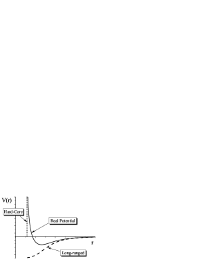
Figure 2: Interaction potentials.

It consists of the long–range component causing attraction and the part leading to strong repulsion at short distances. Such a form of the potential allows the system of nucleons to be modeled with a good accuracy by a set of hard spheres with a certain attractive potential between them, i.e., by a combination of the potentials indicated in Fig. 2 by the vertical dotted and dashed lines. The presence of a hard–core component in nucleons determines the dependence $R\sim A^{1/3}$ for the radius of nuclei, where $A$ is the nuclear mass number. All these considerations lead to the idea of describing matter in the subnuclear range in terms of the excluded–volume approximation (EVA) — a well–known approach in the thermodynamics of gases that allows for the finite size of the system’s components. In the succeeding sections, we will attempt to construct an EVA model that would be thermodynamically self–consistent, would naturally describe systems with a large number of components with different sizes, would take into account the component degeneracy effects, and would admit the inclusion of additional (apart from the hard–core one) interactions between particles.

BOLTZMANN GAS

To derive the expressions for the thermodynamic quantities of a Boltzmann gas in the EVA model, let us consider the standard procedure (see, e.g., Landau and Lifshitz 1976) of the particle distribution over the phase space. The system under consideration consists of $M$ types of particles with the total number of particles of each type $N_{n},\ n=1{\div}M$. Each type of particles is divided into $L_{n}$ groups, $N_{n}=\sum_{k=1}^{L_{n}}N_{n}^{k}$, belonging to different regions of the momentum space $G_{n}^{k}=g_{n}d^{3}p_{k}/h^{3}$, where $g_{n}=(2j_{n}{+}1)$ is the degeneracy factor. Let us calculate the total number of states available to such a system. For the first particle of the first type from the first group, $G_{1}^{1}V$ states are available, where $V$ is the system’s volume. For the second particle, the number of states is $G_{1}^{1}(V-\upsilon_{11})$. Here, $\upsilon_{ij}\equiv\frac{\pi}{6}(\sigma_{i}{+}\sigma_{j})^{3}$ is the so–called volume of the shielding sphere and $\sigma_{i}$ is the diameter of the corresponding type of particles. Continuing this procedure, we will obtain the number of states available to the particles of the first type from the first group, $\triangle\Gamma_{1}^{1}$:

$$\triangle\Gamma_{1}^{1}=\frac{G_{1}^{1}V\times G_{1}^{1}(V{-}\upsilon_{11})\times\ldots\times G_{1}^{1}(V{-}(N_{1}^{1}{-}1)\upsilon_{11})}{N_{1}^{1}!},$$ (1)

where the factorial in the denominator emerges, because the particles are identical. The number of available states is $G_{1}^{2}(V{-}\upsilon_{11}N_{1}^{1})$ for the first particle from the second group, $G_{1}^{2}(V{-}\upsilon_{11}N_{1}^{1}{-}\upsilon_{11})$ for the second particle, and so on. In general, the following formula is valid for the number of states:

$$\triangle\Gamma_{n}^{k}=\frac{G_{n}^{k}(V{-}A_{n}^{k}){\times}G_{n}^{k}(V{-}A_{n}^{k}{-}\upsilon_{nn}){\times}{\ldots}{\times}G_{n}^{k}(V{-}A_{n}^{k}{-}\upsilon_{nn}(N_{n}^{k}{-}1))}{N_{n}^{k}!},$$ (2)

$$A_{n}^{k}=\sum\limits_{i=1}^{n-1}\upsilon_{ni}N_{i}+\sum\limits_{j=1}^{k-1}\upsilon_{nn}N_{n}^{j}.$$ (3)

The total number of states for the system is the product $\triangle\Gamma=\prod_{n,k}\triangle\Gamma_{n}^{k}$ and the entropy is defined via its logarithm: $S=k_{\mathrm{b}}\ln\triangle\Gamma=k_{\mathrm{b}}\sum_{n,k}\ln\triangle\Gamma_{n}^{k}$, where $k_{\mathrm{b}}$ is the Boltzmann constant. Using Stirling’s formula, the expression for the logarithm of the number of states can be brought to the form

$$\ln\triangle\Gamma_{n}^{k}=\frac{V{-}A_{n}^{k}}{\upsilon_{nn}}\ln G_{n}^{k}(V{-}A_{n}^{k})-\frac{V{-}A_{n}^{k+1}}{\upsilon_{nn}}\ln G_{n}^{k}(V{-}A_{n}^{k+1})-N_{n}^{k}\ln N_{n}^{k}.$$ (4)

Since the approximation considered here is valid only if the excluded volume is small, the derived expression should be expanded to give

$$S=k_{\mathrm{b}}\sum\limits_{n,k}N_{n}^{k}\ln\frac{G_{n}^{k}Ve}{N_{n}^{k}}-\frac{k_{\mathrm{b}}}{2V}\sum\limits_{i,j}\upsilon_{ij}N_{i}N_{j}.$$ (5)

Here, the first term is the ordinary Boltzmann expression for entropy and the second term is attributable to the excluded–volume effect. In equilibrium, the entropy must have a maximum at fixed values of the numbers of particles of each type $N_{n}=\sum_{k}N_{n}^{k}$ and the total energy of the system $E=\sum_{n,k}N_{n}^{k}\varepsilon_{n}^{k}$, where $\varepsilon_{n}^{k}$ is the energy of the particles of type $n$ belonging to the $k$-th group. The standard Lagrange multiplier method of searching for a minimum by varying $N_{n}^{k}$ leads to the equation

$$k_{\mathrm{b}}\ln\frac{G_{n}^{k}V}{N_{n}^{k}}-\frac{k_{\mathrm{b}}}{V}\sum\limits_{i}\upsilon_{ni}N_{i}+\alpha_{n}+\beta\varepsilon_{n}^{k}=0.$$ (6)

The Lagrange multipliers are nothing but $\alpha_{n}=\mu_{n}/T$ and $\beta=-1/T$, where $\mu_{n}$ is the chemical potential for the particles of type $n$ and $T$ is the temperature. Now, we can ultimately write

$$N_{n}^{k}=G_{n}^{k}\Bigl{(}V{-}\sum_{i}\overline{\upsilon}_{in}N_{i}\Bigr{)}\exp\biggl{(}-\frac{\varepsilon_{n}^{k}}{k_{\mathrm{b}}T}+\frac{\mu_{n}}{k_{\mathrm{b}}T}-\frac{1}{V}\sum_{i}\overline{\upsilon}_{ni}N_{i}\biggr{)}.$$ (7)

Here, we introduced the quantities $\overline{\upsilon}_{ij}$ satisfying the condition $\overline{\upsilon}_{ij}+\overline{\upsilon}_{ji}=\upsilon_{ij}$. In the linear (in excluded volume) approximation, it does not matter whether we write the correction determined by it as a factor in front of the exponential in Eq. $(\ref{N-Bolzmann})$ or as an addition to the chemical potential. However, the need for expanding the domain of applicability and comparison with other approaches force us to write this expression precisely in this form. For identical particles, $\overline{\upsilon}_{ii}=\upsilon_{ii}/2$, which corresponds to the well-known approximation of an effective excluded volume equal to quadruple the intrinsic particle volume. In addition, there exist other constraints on the choice of $\overline{\upsilon}_{ij}$ to be discussed in detail below. However, certain freedom in choosing the expression for $\overline{\upsilon}_{ij}$ remains. Summing Eq. $(\ref{N-Bolzmann})$ over $k$, we will obtain the system of equations relating the numbers of particles to the temperature and chemical potentials. The sum $\sum_{k}\varepsilon_{n}^{k}N_{n}^{k}$ defines the energy of the $n$-th type of particles. Substituting the expression for $N_{n}^{k}$ into Eq. $(\ref{S-Bolzmann})$ give the expression for entropy and so on.

THE GENERAL CASE

The simple scheme of allowance for the finite size of particles described in the preceding section is unsatisfactory for several reasons. First, it was formulated only for Boltzmann statistics. Second, it is unclear how to take into account other interactions that are not described by the EVA in it. And, most importantly, it becomes inapplicable even at $V=N_{n}\overline{\upsilon}_{nn}$ (we consider one type of particles). Let us introduce the concept of a packing fraction $\eta=\sum_{i}\textbf{v}_{i}n_{i}$, where $\textbf{v}_{i}$ is the intrinsic volume of the particles and $n_{i}$ is their number density. Obviously, this quantity is the ratio of the volume occupied by the particles to the total volume. The equations from the preceding section are then seen to become inapplicable at $\eta=0.25$. Meanwhile, it is well known that the closest packing of spheres with the same size is achieved in a face-centered cubic lattice at $\eta=\pi/3\sqrt{2}\approx 0.74$. Moreover, numerical simulations show that the phase transition to crystalline order in a system of hard spheres occurs at $\eta\approx 0.6$. The cause of such an overestimation of the excluded-volume effect in the above analysis is clear: we assumed that each particle reduced the space available to other particles by a value equal to the volume of the shielding sphere. For identical particles, this is quadruple the particle volume: the excluded volume for two particles is $\frac{\pi}{6}(2\sigma_{n})^{3}$. Meanwhile, this is true only in the limit of low number densities: the effective volume per particle must decrease as they increase, i.e., the excluded volume must be a function of the number densities of the system’s components. Below, we will attempt to construct a phenomenological theory that would take these requirements into account and would be free from these shortcomings.

We will assume that all particles are fermions. For subnuclear-density supernova matter of interest to us, this is always the case: the free neutrons and protons are described by Fermi statistics, while the nuclei are far from degeneracy and are a Boltzmann gas (the limiting case of Fermi statistics). The expression for the logarithm of the number of states for an ideal Fermi gas is (the notation is the same as that used above)

$$\ln\triangle\Gamma_{n}^{k}=G_{n}^{k}V\ln G_{n}^{k}V-\left[G_{n}^{k}V-N_{n}^{k}\right]\ln(G_{n}^{k}V-N_{n}^{k})-N_{n}^{k}\ln N_{n}^{k}.$$ (8)

The substitution that we make to take into account the excluded-volume effect is natural: $V\rightarrow V{-}\upsilon_{n}$, with $\upsilon_{n}=\upsilon_{n}(N_{1},N_{2},\ldots,N_{M})$ being a function of the numbers of particles for all components of the system. To begin with, let us calculate the necessary derivatives:

$$\!\left(\!\frac{\partial\ln\triangle\Gamma_{n}^{k}}{\partial N_{n}^{k}}\!\right)_{\!\!\upsilon_{n}}\! =\ln\left[G_{n}^{k}(V{-}\upsilon_{n}){-}N_{n}^{k}\right]-\ln N_{n}^{k},$$ (9)

$$\!\left(\!\frac{\partial\ln\triangle\Gamma_{n}^{k}}{\partial\upsilon_{n}}\!\right)_{\!\!N_{n}^{k}}\! =-G_{n}^{k}\ln G_{n}^{k}(V{-}\upsilon_{n})+G_{n}^{k}\ln\left[G_{n}^{k}(V{-}\upsilon_{n}){-}N_{n}^{k}\right].$$ (10)

The derivative of the entropy with respect to $N_{n}^{k}$ is

$$\quad\quad\quad\!\left(\!\frac{\partial S}{\partial N_{n}^{k}}\!\right)_{\!\!}\!=k_{\mathrm{b}}\!\left(\!\frac{\partial\ln\triangle\Gamma_{n}^{k}}{\partial N_{n}^{k}}\!\right)_{\!\!\upsilon_{n}}\!\!+k_{\mathrm{b}}\!\sum_{p,j}\!\left(\!\frac{\partial\ln\triangle\Gamma_{p}^{j}}{\partial\upsilon_{p}}\!\right)_{\!\!N_{p}^{j}}\!\!\left(\!\frac{\partial\upsilon_{p}}{\partial N_{n}}\!\right)_{\!\!}\!.$$ (11)

The variational principle $\delta(S+\sum_{n}\alpha_{n}N_{n}+\beta E)=0$ gives

$$k_{\mathrm{b}}\ln\left[\frac{G_{n}^{k}(V{-}\upsilon_{n}){-}N_{n}^{k}}{N_{n}^{k}}\right]+\alpha_{n}+\beta\varepsilon_{n}^{k}+\\ +k_{\mathrm{b}}\sum_{p}\!\left(\!\frac{\partial\upsilon_{p}}{\partial N_{n}}\!\right)_{\!\!}\!\sum_{i}G_{p}^{i}\ln\left[\frac{G_{p}^{i}(V{-}\upsilon_{p}){-}N_{p}^{i}}{G_{p}^{i}(V{-}\upsilon_{p})}\right]=0.$$ (12)

Making the identification of $\alpha_{n}=\mu_{n}/T$ and $\beta=-1/T$, we obtain

$$N_{n}^{k}=\frac{G_{n}^{k}(V{-}\upsilon_{n})}{1{+}\exp\left[(\varepsilon_{n}^{k}-\widetilde{\mu}_{n})/k_{\mathrm{b}}T\right]},$$ (13)

$$\widetilde{\mu}_{n}=\mu_{n}+k_{\mathrm{b}}T\sum_{p}\!\left(\!\frac{\partial\upsilon_{p}}{\partial N_{n}}\!\right)_{\!\!}\!\sum_{i}G_{p}^{i}\ln\left[\frac{G_{p}^{i}(V{-}\upsilon_{p}){-}N_{p}^{i}}{G_{p}^{i}(V{-}\upsilon_{p})}\right].$$ (14)

We will introduce a new designation $\widehat{\upsilon}_{n}\equiv\upsilon_{n}/V$ and will mark the functions pertaining to an ideal Fermi gas by the superscript $\mathrm{id}$. Summing Eq. (13) over $k$ yields

$$N_{n}=\left(1{-}\widehat{\upsilon}_{n}\right)N_{n}^{\mathrm{id}}(T,\widetilde{\mu}_{n}).$$ (15)

Substituting Eq. $(\ref{Nnk})$ for $N_{n}^{k}$ into the double sum of Eq. $(\ref{mu-general})$ for the chemical potential, we will find that

$$\widetilde{\mu}_{n}=\mu_{n}-\sum_{p}\!\left(\!\frac{\partial\widehat{\upsilon}_{p}}{\partial n_{n}}\!\right)_{\!\!}\!P_{p}^{\mathrm{id}}(T,\widetilde{\mu}_{p}),$$ (16)

where $P_{p}^{\mathrm{id}}(T,\widetilde{\mu}_{p})$ is the pressure of an ideal Fermi gas as a function of the temperature and chemical potential, while $n_{n}$is the number density of the $n$-th mixture component. It is now easy to derive the expressions for the thermodynamic potentials:

$$E=\sum_{n}(1{-}\widehat{\upsilon}_{n})E_{n}^{\mathrm{id}}(T,\widetilde{\mu}_{n})=\sum_{n}N_{n}\textbf{E}_{n}^{\mathrm{id}}(T,\widetilde{\mu}_{n}),$$ (17)

where we introduced the energy per particle $\textbf{E}_{n}^{\mathrm{id}}=E^{\mathrm{id}}_{n}/N_{n}$. Similarly,

$$S =\sum_{n}(1{-}\widehat{\upsilon}_{n})S_{n}^{\mathrm{id}}(T,\widetilde{\mu}_{n})=\sum_{n}N_{n}\textbf{S}_{n}^{\mathrm{id}}(T,\widetilde{\mu}_{n}),$$ (18)

$$F =\sum_{n}(1{-}\widehat{\upsilon}_{n})F_{n}^{\mathrm{id}}(T,\widetilde{\mu}_{n})=\sum_{n}N_{n}\textbf{F}_{n}^{\mathrm{id}}(T,\widetilde{\mu}_{n}),$$ (19)

where $F$ is the system’s free energy. We can now determine the pressure

$$P=\frac{1}{V}\Bigl{(}\sum_{n}\mu_{n}N_{n}{-}F\Bigr{)}=\sum_{n}\!\left[1{-}\widehat{\upsilon}_{n}{+}\!\sum_{i}\!\left(\!\frac{\partial\widehat{\upsilon}_{n}}{\partial n_{i}}\!\right)_{\!\!}\!n_{i}\right]P_{n}^{\mathrm{id}}(T,\widetilde{\mu}_{n}).$$ (20)

Formulas (15)–(20) completely describe the thermodynamics of matter in terms of the approach to the EVA under consideration.

It can be shown that this EVA description provides a thermodynamically consistent description of the system (i.e., an automatic fulfilment of all thermodynamic relations) for any dependence $\widehat{\upsilon}_{n}$ on the number densities of the mixture components.

Thus, the approach considered provides a convenient tool for investigating the thermodynamics of nonideal matter in terms of which interaction models can be constructed by choosing the form of the excluded–volume function $\widehat{\upsilon}_{n}$ in conformity with the problem under consideration. For example, let us take an approximation where the excluded volume is the same for all types of particles and is just equal to the volume occupied by these particles: $\widehat{\upsilon}_{n}=\sum_{i}\textbf{v}_{i}n_{i}$, where $\textbf{v}_{i}$ is the intrinsic volume of the particles of type $i$ and $n_{i}$ is their number density. In this case,

$$P=\sum_{n}P_{n}^{\mathrm{id}}(T,\widetilde{\mu}_{n})=P^{\mathrm{id}}(T,\{\widetilde{\mu}_{n}\}),\quad\widetilde{\mu}_{n}=\mu_{n}{-}\textbf{v}_{n}P^{\mathrm{id}}(T,\{\widetilde{\mu}_{n}\}),$$ (21)

i.e., we obtained the EVA description that was proposed by Rischke et al. (1991) and that is widely used in describing the reactions with heavy ions (see, e.g., Hung and Shuryak 1998; Gorenstein et al. 1996).

INTERACTION EFFECTS

The above EVA scheme can be supplemented by the mechanism of allowance for additional interactions between particles. It is well known that a fairly wide class of interactions can be described in the formalism of free energy where the free energy of a system $F(T,V,\{N_{i}\})$ is represented as the sum of the system’s free energy without any interaction $F^{\mathrm{id}}(T,V,\{N_{i}\})$ and the additional term $\triangle F(T,V,\{N_{i}\})$ attributable to the interaction: $F=F^{\mathrm{id}}{+}\triangle F$. Using this approach, the system’s free energy in our case should be written as

$$F=\sum_{n}(1{-}\widehat{\upsilon}_{n})F_{n}^{\mathrm{id}}(T,\widetilde{\mu}_{n})+\triangle F(T,V,\{N_{i}\}).$$ (22)

Introducing the additional term describing the interaction into the free energy allows the corresponding changes in the remaining quantities to be obtained in a thermodynamically consistent way:

$$\widetilde{\mu}_{n} \Rightarrow\widetilde{\mu}_{n}+\frac{1}{V}\!\left(\!\frac{\partial\triangle F}{\partial n_{n}}\!\right)_{\!\!V,T}\!$$ (23)

$$P \Rightarrow P+\frac{1}{V}\left[\sum_{i}n_{i}\!\left(\!\frac{\partial\triangle F}{\partial n_{i}}\!\right)_{\!\!V,T}\!\!\!-\triangle F\right]$$ (24)

$$S \Rightarrow S-\!\left(\!\frac{\partial\triangle F}{\partial T}\!\right)_{\!\!V,\{N_{i}\}}\!$$ (25)

$$E \Rightarrow E+\triangle F-T\!\left(\!\frac{\partial\triangle F}{\partial T}\!\right)_{\!\!V,\{N_{i}\}}\!$$ (26)

These formulas describe the procedure of allowance for additional interactions in the approach under consideration.

CONNECTION WITH THE HARD–SPHERE MODEL

To concretize the form of the excluded–volume function $\widehat{\upsilon}_{n}$, let us consider the so-called hard–sphere approximation, i.e., the model of an ideal gas of particles interacting through the potential

$$U_{ij}(r)=\left\{\begin{aligned} 0&,\ \mbox{при}\ r\geq(\sigma_{i}{+}\sigma_{j})/2,\\ {+}\infty&,\ \mbox{при}\ r<(\sigma_{i}{+}\sigma_{j})/2,\end{aligned}\right.$$ (27)

where $r$ is the separation between the mixture components and $\sigma_{i}$ are the particle diameters. Numerous analytical results were obtained in this approximation and its application to the description of liquid properties was considered. In recent years, the study has also been carried out using numerical simulations. Therefore, it is natural to associate our approach in this limit with the above theory and to try to determine the as yet unknown quantities. For this purpose, we will set $\triangle F=0$ and will assume that all particles are Boltzmann ones.

The Single–Component Case

An important parameter of the hard–sphere model is $\Gamma\equiv P/\left(k_{\mathrm{b}}T\!\sum_{i}n_{i}\right)$. Its deviation from unity characterizes the degree of nonideality of the system. In the single–component case, this quantity depends only on the packing fraction $\eta$. Different analytical approaches give different values for this quantity. The following expressions are the best known ones:

$$\Gamma_{\mathrm{PY}}=\frac{1{+}2\eta{+}3\eta^{2}}{(1{-}\eta)^{2}},\quad\Gamma_{\mathrm{L}}=\frac{1{+}\eta{+}\eta^{2}}{(1{-}\eta)^{3}},\quad\Gamma_{\mathrm{CS}}=\frac{1{+}\eta{+}\eta^{2}{-}\eta^{3}}{(1{-}\eta)^{3}}.$$ (28)

The first two were derived by Lebowitz (1964) based on the solution of the Percus–Yevick equation for the radial distribution function; the last was derived by Carnahan and Starling (1969) and is currently considered more accurate. In the subsequent applications, we will use precisely this expression.

Let us now consider the expression for the pressure in our description:

$$P=\left[1{-}\widehat{\upsilon}{+}n\!\left(\!\frac{\partial\widehat{\upsilon}}{\partial n}\!\right)_{\!\!}\!\ \right]P^{\mathrm{id}}(T,\widetilde{\mu})=\left[1{-}\widehat{\upsilon}{+}n\!\left(\!\frac{\partial\widehat{\upsilon}}{\partial n}\!\right)_{\!\!}\!\ \right]\frac{nkT}{1{-}\widehat{\upsilon}},$$ (29)

whence it follows that

$$1{+}\frac{\eta}{1{-}\widehat{\upsilon}}\!\left(\!\frac{\partial\widehat{\upsilon}}{\partial\eta}\!\right)_{\!\!}\!=\Gamma(\eta)\ \ \Rightarrow\ \ \widehat{\upsilon}(\eta)=1{-}\exp\biggl{(}{-}\!\!\int\limits_{0}^{\eta}\!\frac{\Gamma(x){-}1}{x}\ dx\biggr{)}.$$ (30)

Thus, in the single-component case, we determined the form of the dependence of the relative excluded volume $\widehat{\upsilon}$ on particle number density that remained unknown. In the limit of low number densities, $\Gamma(\eta)\approx 1{+}4\eta$ and, hence, $\widehat{\upsilon}(\eta)\approx 4\eta$, i.e., the effective excluded volume is equal to quadruple the intrinsic particle volume, in complete agreement with the previously reached conclusions.

The Multicomponent Case

It should be noted at once that since there is no universally accepted approach to describing a multicomponent system of hard spheres, the approximation presented below is not the only possible one. On the other hand, this may be considered as a definite plus, because the breadth of the already described scheme, when necessary, can accommodate new data on complex properties of such systems. Our subsequent consideration will be associated with the work by Lopez de Haro et al. (2008), some of whose propositions we will use.

For convenience, let us introduce a set of quantities $\psi_{n}$ according to the definition: $e^{-\psi_{n}}\equiv 1{-}\widehat{\upsilon}_{n}$. Obviously, $\psi_{n}$ are nonnegative. Now, we will make the first assumption that $\psi_{n}=\psi_{n}(\eta,\langle\sigma^{k}\rangle)$, i.e., the number densities of the components can enter into the expression for $\psi_{n}$ only via the packing fraction $\eta$ and the means $\langle\sigma^{k}\rangle\equiv\sum_{i}\sigma_{i}^{k}n_{i}/\sum_{i}n_{i}$.

Let us now list the conditions that our model of a multicomponent system should satisfy:

1. If the diameter of some component is zero, $\sigma_{k}=0$, then these particles must be described by the formulas for an ideal (in the sense that there is no interaction) gas, $\widetilde{\mu}_{k}=\mu_{k}$, but located in a reduced volume $V^{*}=V(1{-}\eta)$.

2. The limit of low number densities described above in the ‘‘Boltzmann Gas’’ Section must hold, i.e.

   $$\widehat{\upsilon}_{n}+\sum_{i}\!\left(\!\frac{\partial\widehat{\upsilon}_{i}}{\partial n_{n}}\!\right)_{\!\!}\!\ n_{i}=\frac{\pi}{6}\sum_{i}n_{i}\sigma_{in}^{3},\quad\sigma_{in}\equiv\sigma_{i}{+}\sigma_{n}.\vspace{-1.cm}$$ (31)

3. If the diameters of all particles are identical, then all must be reduced to the single-component case $\Gamma(\{n_{i}\})=\Gamma_{\mathrm{sc}}(\eta)$.

These conditions impose moderately stringent constraints on the form of the function $\psi_{n}$, leaving a large room for various options. Given that in the limit of low number densities $\psi_{n}\approx\widehat{\upsilon}_{n}$, we will seek $\psi_{n}$ in the form

$$\psi_{n}=\frac{\pi}{6}\sum_{i}n_{i}\widehat{\sigma}_{ni}^{3}G(\eta,z_{ni}),\quad z_{ni}=2\frac{\sigma_{n}\sigma_{i}}{\sigma_{ni}}\frac{\langle\sigma^{2}\rangle}{\langle\sigma^{3}\rangle}.$$ (32)

The quantity $\frac{\pi}{6}\widehat{\sigma}_{ni}^{3}$ means the effective volume unavailable to the $n$-th particle due to its interaction with the $i$-th one. The function $G(\eta,z_{ni})\rightarrow 1$ when $\eta\rightarrow 0$. The introduction of $z_{ni}$ is justified by the comparison with some works on multicomponent systems (see Lopez de Haro et al. (2008) and references therein). For our purposes, it will suffice to use the linear expansion $G(\eta,z_{ni})=g_{1}(\eta){+}z_{ni}g_{2}(\eta)$ by assuming that the term $g_{1}$ plays a major role at low number densities. Allowance for additional conditions can require including the next terms of the expansion in $G(\eta,z_{ni})$ in $z_{ni}$, but we will restrict ourselves to the linear approximation.

Consider condition 1 and let $\sigma_{n}=0$. The expressions for the excluded volume and the chemical potential will be written as

$$1{-}\widehat{\upsilon}_{n}=1{-}\eta=\exp\!\left({-}\frac{\pi}{6}g_{1}(\eta)\sum_{i}\widehat{\sigma}_{ni}^{3}n_{i}\right),$$ (33)

$$\widetilde{\mu}_{n}=\mu_{n}-\frac{\pi}{6}g_{1}(\eta)\sum_{i}\widehat{\sigma}_{in}^{3}n_{i}.$$ (34)

Hence and from the meaning of $\widehat{\sigma}_{ij}$ it follows that

$$\widehat{\sigma}_{ni}=\sigma_{i},\ \mbox{а}\ \ \widehat{\sigma}_{in}=0\ \mbox{при}\ \sigma_{n}=0,$$ (35)

$$g_{1}(\eta)=-\frac{\ln(1{-}\eta)}{\eta}.$$ (36)

Let us now pass to condition 31. Remembering that $g_{\mathrm{1}}(\eta)$ plays a major role at low densities, we can write $\widehat{\upsilon}_{n}\approx\frac{\pi}{6}\sum_{i}n_{i}\widehat{\sigma}_{ni}^{3}$. Condition $(\ref{Low-Formula})$ can then be rewritten as

$$\widehat{\sigma}_{ni}^{3}+\widehat{\sigma}_{in}^{3}=\sigma_{in}^{3}.$$ (37)

Now, we should choose the specific form of $\widehat{\sigma}_{in}$, satisfying the conditions listed above. We could have used the expression from Gorenstein et al. (1999), who used the relation

$$\widehat{\sigma}_{ni}^{3}=\frac{\sigma_{i}^{3}\sigma_{ni}^{3}}{\sigma_{i}^{3}{+}\sigma_{n}^{3}},$$ (38)

However, in this case, $\psi_{n}$ cannot be represented as $\psi_{n}=\psi_{n}(\eta,\langle\sigma^{k}\rangle)$. Therefore, we propose the dependence

$$\widehat{\sigma}_{ni}^{3}=\sigma_{i}\sigma_{ni}^{2}.$$ (39)

Note once again that these relations are not the only possible ones; they are only the simplest ones satisfying the necessary conditions.

Now, it remains to use requirement 3 to find $g_{2}(\eta)$. When the diameters of all particles are identical, $\psi_{n}=4\eta\left[g_{1}(\eta){+}g_{2}(\eta)\right]$. Substituting this expression into the formula for $\Gamma$ yields

$$g_{2}(\eta)=\frac{1}{4\eta}\int\limits_{0}^{\eta}\left[\Gamma_{\mathrm{sc}}(x){-}\frac{1{+}3x}{1{-}x}\right]\frac{dx}{x},$$ (40)

where $\Gamma_{\mathrm{sc}}(\eta)$ is the expression for $\Gamma$ in the single–component case, for example, one of Eqs. (28). Now, it remains to bring all formulas together and to write explicit expressions for $\psi_{n}$ and $\Gamma$ as a function of $\eta$ and $\langle\sigma^{k}\rangle$.

$$\frac{\psi_{n}}{\eta}=\left[1{+}2\sigma_{n}\frac{\langle\sigma^{2}\rangle}{\langle\sigma^{3}\rangle}{+}\sigma_{n}^{2}\frac{\langle\sigma\rangle}{\langle\sigma^{3}\rangle}\right]g_{1}(\eta)+2\sigma_{n}\frac{\langle\sigma^{2}\rangle}{\langle\sigma^{3}\rangle}\left[1{+}\sigma_{n}\frac{\langle\sigma^{2}\rangle}{\langle\sigma^{3}\rangle}\right]g_{2}(\eta).$$ (41)

Substituting this expression into the formula for $\Gamma$ and using the derived expressions for the functions $g_{1}(\eta)$ and $g_{2}(\eta)$, we will obtain

$$\Gamma=\frac{1}{1{-}\eta}+\frac{\langle\sigma\rangle\langle\sigma^{2}\rangle}{2\langle\sigma^{3}\rangle}\left\{\left[\Gamma_{\mathrm{sc}}(\eta){-}\frac{1}{1{-}\eta}\right]\left(1{+}\frac{\langle\sigma^{2}\rangle^{2}}{\langle\sigma\rangle\langle\sigma^{3}\rangle}\right)+\frac{3\eta}{1{-}\eta}\left(1{-}\frac{\langle\sigma^{2}\rangle^{2}}{\langle\sigma\rangle\langle\sigma^{3}\rangle}\right)\right\}.$$ (42)

These expressions exactly correspond to the formula for $\Gamma$, derived in the same approximation by Lopez de Haro et al. (2008).

Thus, using Eq. (41), we were able to relate $\psi_{n}$ and, via it $\widehat{\upsilon}_{n}$ to the number densities and diameters of the particles constituting the system. However, our formulas are applicable not only for an ideal gas but also for degenerate particles and when additional interactions are present in the system.

MATTER IN THE SUBNUCLEAR RANGE

To derive the equation of state in the subnuclear range that provides the phase transition to uniform nuclear matter at densities $\rho\sim 10^{14}\ \mbox{g$\,$cm${}^{-3}$}$, it is necessary to add the long-range attractive interaction potential to the short–range repulsive potential described in our approach by the excluded-volume effect. The well–known Yukawa potential $V(r)\propto e^{-\lambda r}/r$, where $\lambda$ is determined by the pion Compton wavelength $l_{\pi}=1/\lambda\approx 1.41\leavevmode\nobreak\ \mbox{fm}$, is used to describe the interaction of isolated nucleons at great distances. In reality, the interaction between nucleons in the range of nuclear densities is not reduced to the sum of pair interactions. This forces one to introduce the concept of the so-called effective interaction potential whose form and parameters are chosen in such a way as to reproduce the properties of uniform nuclear matter, such as the saturation density $n_{\mathrm{b}}\approx 0.16\ \mbox{fm}^{-3}$, the binding energy per nucleon $B\approx-16\leavevmode\nobreak\ \mbox{MeV}$ etc. For example, the effective Seyler–-Blanchard potential is the product of a Yukawa potential with a parameter $1/\lambda\approx 0.6\ \mbox{fm}$ by a function dependent both on the local matter density and on the momenta of the interacting nucleons (for more detail, see Myers and Swiatecki 1969).

We will use a Yukawa potential whose parameters are chosen from the condition for consistency with the equation of state for nuclear matter. This form of the potential was chosen only because of its simplicity in order to demonstrate the efficiency of the approach being described. As we will see below, in general, the results are rather sensitive to the parameters of the potential and choosing it to obtain realistic results is a nontrivial problem.

The additional complexity is that we should include the interactions between free nucleons and between nuclei in the description. This question is considered in the Appendix, where the specific values of parameters used in our calculations are also given.

RESULTS AND DISCUSSION

We will apply the developed approach to describe the subnuclear density range for supernova matter under NSE conditions. In the subsequent figures, unless specified otherwise, the temperature $T=5\leavevmode\nobreak\ \mbox{MeV}$ and $\mbox{$Y_{\mathrm{e}}$}=1/3$ everywhere. The results of the model including only the excluded-volume effect are marked as ‘‘EV’’, while those of the model that, apart from this effect, includes the long-range potential are marked as ‘‘EV+LRA’’.

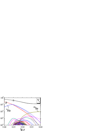
Figure 3: (Color online) Chemical composition of matter at $T=5\leavevmode\nobreak\ \mbox{MeV}$ and $\mbox{$Y_{\mathrm{e}}$}=1/3$, the EV model.

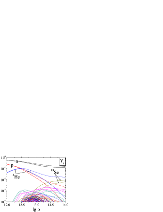
Figure 4: (Color online) Chemical composition of matter at $T=5\leavevmode\nobreak\ \mbox{MeV}$ and $\mbox{$Y_{\mathrm{e}}$}=1/3$, model $\mathrm{EV}{+}\mathrm{LRA}$

Figure 3 shows the equilibrium chemical composition of matter as a function of the density. The solid lines represent the calculation with ideal matter; the dashed lines indicate the result of the EV model. Similar data are presented in Figure 4, with the only difference that the dotted lines indicate the result of our calculation according to the EV+LRA model.

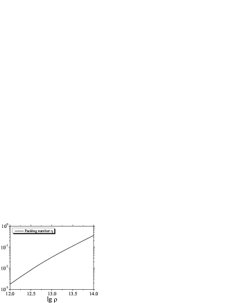
Figure 5: Packing fraction $\eta$

Figure 5 shows the calculated packing fraction $\eta$ under the same conditions. As we see, the excluded–volume effect per se has a weak influence on the equilibrium mass fractions up to $\rho=10^{14}\leavevmode\nobreak\ \mbox{g\,cm${}^{-3}$}$, although the packing fraction reaches a significant value here, $\eta\approx 0.4$. Allowance for the long–range part of the potential gives a considerably stronger effect: the number density of free nucleons and $\alpha$-particles increases; the number density of heavy nuclei, in particular, the neutron-rich selenium isotopes that are representatives of all neutron-rich nuclei in our set of nuclides, decreases (for more detail, see Nadyozhin and Yudin 2004). Thus, first, the long–range component of the effective nucleon–nucleon interaction potential itself and, second, the method for generalizing this interaction to nuclei are important for a proper description of the subnuclear range. the widely used mean–nucleus models, a decrease in the surface energy of the nucleus due to the medium’s effects corresponds to this interaction. Our method is presented in the Appendix.

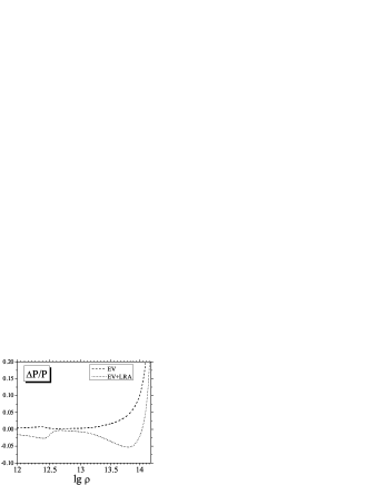
Figure 6: Relative change in the pressure of matter.

Figure 6 shows the relative change in pressure $(P{-}P^{\mathrm{id}})/P^{\mathrm{id}}$, where $P^{\mathrm{id}}$ is the pressure of ideal matter. The dashed and dotted lines indicate the EV and EV+LRA models, respectively. The non–monotonic behavior of the curves at $\lg\rho\approx 12.5$ is associated with the change in equilibrium chemical composition under the influence of interaction. At $\rho\sim 10^{14}\leavevmode\nobreak\ \mbox{g\,cm${}^{-3}$}$ the pressure in both models rises sharply.

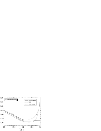
Figure 7: Adiabatic indices for matter.

Figure 7 shows the behavior of the adiabatic index $\gamma\equiv\left(\partial\ln P/\partial\ln\rho\right)_{S}$ for ideal matter (solid line), the EV model (dashed line), and the EV+LRA model (dotted line). As would be expected, the EV model makes the matter ‘‘stiffer’’ in the entire density range, while the long–range potential of the EV+LRA model causes $\gamma$ to be reduced in the range of low densities. At $\rho\gtrsim 10^{14}$ the equation of state in the excluded-volume models becomes very ‘‘stiff’’. The phase transition to uniform nuclear matter to be discussed in the next section should occur in this range.

The Phase Transition

Naturally, only the equation of state defined in the entire domain of thermodynamic parameters of interest to us and containing the low– and high–density phases as their limiting cases can give an absolutely proper description of the phase transition. The EVA is a low–density approximation of the real equation of state and cannot be applied at excessively high densities. However, as we will show below, the EVA can be used in this capacity in the phase equilibrium equations (equality between the pressures and chemical potentials of the phases) provided that the equation of state for uniform nuclear matter (as such we use the results of the approach by Lattimer and Swesty (1991)) is used for the high–density phase. In this case, the parameters of both phases should be reconciled, which is a separate nontrivial problem. In fact, the procedure described above provides a thermodynamically proper joining of the two equations of state. In particular, this approach proved to be good in our hydrodynamic simulations of gravitational collapse.

Figure 8: Фазовая диаграмма вещества

Figure 8 shows the phase diagram for matter calculated using the procedure described above with the EV+LRA model for the equation of state for the low–density phase. The dashed lines indicate the boundary between the low-density phase and the region of mixed states; the solid lines indicate the boundary between the mixed states and the high–density phase (uniform nuclear matter). The numbers with arrows indicate the leptonic charges $Y_{\mathrm{e}}$ for each pair of lines: the thick, thinner, and thinnest lines correspond to $\mbox{$Y_{\mathrm{e}}$}=1/2$, $\mbox{$Y_{\mathrm{e}}$}=1/3$ and $\mbox{$Y_{\mathrm{e}}$}=1/4$ respectively. As the temperature rises, the lines of the phase boundaries converge, i.e., the equations of state for the phases become increasingly close. On the real phase diagram for matter, there must be a critical point with a certain temperature $T_{\mathrm{c}}$ above which the phases are indistinguishable in this region.

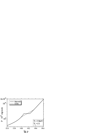
Figure 9: Pressure during the phase transition (see the text).

Figure 9 shows the behavior of the matter pressure during the phase transition. The solid line with a characteristic plateau $P=\mathrm{const}$ corresponds to the ordinary description of the phase transition according to Maxwell’s approach. The latter requires that the pressures and chemical potentials of the phases be equal in the domain of their existence, with each phase being considered electrically neutral. Gibbs’s approach, whose result is indicated by the dotted line, allows the phases to have an uncompensated charge, providing only global electrical neutrality. As we see, $\partial P/\partial\rho>0$, in Gibbs’s approach in the region of mixed states, but this region itself is wider. The phase diagram presented above was calculated in accordance with Maxwell’s ordinary approach.

CONCLUSIONS

The general approach to the EVA developed here can serve as a tool for investigating the extreme states of matter. Different thermodynamically consistent models for the equation of state can be obtained by choosing different forms of the excluded–volume function $\widehat{\upsilon}_{n}$ and the corresponding additional interaction potential.

Using this EVA method, it turned out to be possible to reproduce the results of the hard–sphere model in the Boltzmann limit. This approach is apparently adequate for describing a multicomponent mixture of free nucleons and nuclei under NSE conditions, i.e., the case of supernova matter at subnuclear densities. It can be used not only to study the thermodynamic properties of matter but also to obtain detailed information about its chemical composition. This is a serious advantage of our approach over the popular mean-nucleus models. For example, the nucleosynthesis problems can be solved by using only this type of equations of state.

In addition, we showed that based on this approach to the EVA, we can obtain the phase transition to uniform nuclear matter and, hence, use this equation of state in hydrodynamic simulations of supernova explosions.

APPENDIX

THE INTERACTION OF NUCLEI

Let the interaction energy between two nucleons of a certain type, for example, an $n{-}p$, separated by a distance $r$ be $V_{\mathrm{Y}}(r)=Ye^{-\lambda r}/\lambda r$. The interaction energy between one nucleon $(n)$ and nucleons of a given type $(p)$ in the nucleus will then be

$$E_{\mathrm{int}}=\int V_{\mathrm{Y}}(r)\rho(r)d^{3}r,\quad N=\int\limits_{0}^{R}4\pi r^{2}\rho(r)dr,$$

where $N$ is the number of nucleons of the type under consideration in the nucleus, $R$ is its radius, $\rho(r)$ is the density of the distribution of nucleons in the nucleus, and the distribution itself is assumed to be spherically symmetric. The integration in the formula for $E_{\mathrm{int}}$ is over the entire nucleus volume. We obtain

$$E_{\mathrm{int}}=\int\limits_{0}^{R}\!\!\int\limits_{0}^{\pi}V_{\mathrm{Y}}(l)2\pi r^{2}\rho(r)dr\sin\theta d\theta=NV_{\mathrm{Y}}(L)G_{\rho}(\lambda,R).$$

Here, $l=\sqrt{L^{2}{+}r^{2}{-}2Lr\cos\theta}$, $L$ is the distance between the nucleon and the nucleus center, and

$$G_{\rho}(\lambda,R)=\frac{1}{\lambda}\left[\int\limits_{0}^{R}\rho(r)r\sinh(\lambda r)dr\right]\left[\int\limits_{0}^{R}\rho(r)r^{2}dr\right]^{-1}$$

Thus, the interaction between a nucleon and a uniformly ‘‘charged’’ nucleus is described by the same Yukawa potential, only with the corrected factor $G_{\rho}(\lambda,R)$. Here, there is an analogy with the interaction via a Coulomb (or gravitational) potential, where a uniformly charged sphere is equivalent to an equal (in magnitude) point charge placed at its center (see also Azam and Gowda 2005). Below, for simplicity, we will assume that the density of nucleons in the nucleus is constant. As a result, $G_{\rho}(\lambda,R)$ transforms into $G(\lambda R)$, where

$$G(x)=\frac{3}{x^{2}}\left[\cosh(x)-\frac{\sinh(x)}{x}\right],\quad G(0)=1.$$

Since the potential has the Yukawa form as before, it is not difficult to write out the interaction energy between two nuclei separated by a distance $l$ in the final form; it is only necessary to take into account the fact that the $n{-}n$ and $p{-}p$ pairs interact identically, while the interaction of the $p{-}n$ differs from them: $Y_{\mathrm{nn}}=Y_{\mathrm{pp}}\neq Y_{\mathrm{np}}$.

$$E_{\mathrm{int}} =\frac{e^{-\lambda l}}{\lambda l}P_{1,2}G(\lambda R_{1})G(\lambda R_{2}),$$

$$P_{12} =Y_{\mathrm{nn}}(N_{1}N_{2}+Z_{1}Z_{2})+Y_{\mathrm{np}}(N_{1}Z_{2}+N_{2}Z_{1}),$$

where $N$ and $Z$ are the numbers of neutrons and protons in the nucleus, respectively. Now, it is easy to write the expression for the total energy per unit volume of the (free nucleons + nuclei) system:

$$E_{\mathrm{tot}}=\frac{1}{2}\sum\limits_{i,j}n_{i}n_{j}\!\!\int\limits_{R_{i}+R_{j}}^{\infty}\!\!E_{\mathrm{int}}d^{3}L=\\ =\frac{2\pi}{\lambda^{3}}\sum\limits_{i,j}n_{i}n_{j}P_{ij}\ G(\lambda R_{i})G(\lambda R_{j})e^{-\lambda(R_{i}+R_{j})}[1{+}\lambda(R_{i}{+}R_{j}))],$$

where $n_{i}$ and $n_{j}$ are the number densities of the components. It is easy to determine $Y_{\mathrm{nn}}{=}Y_{\mathrm{pp}}$ and $Y_{\mathrm{np}}$ by comparing this expression with the formula for the energy of uniform nuclear matter (see Lattimer and Swesty 1991). We take the parameter $\lambda$ to be $0.95\ \mbox{fm}$ and the radii of the nuclei and nucleons to be $R_{\mathrm{A,Z}}=1.16A^{1/3}\ \mbox{fm}$ and $R_{\mathrm{n}}=R_{\mathrm{p}}=0.8\ \mbox{fm}$, respectively.

ACKNOWLEDGMENTS

I wish to thank D.K. Nadyozhin for numerous helpful discussions of the questions considered. This work was supported by an SNSF grant (SCOPES project IZ73Z0-128180/1) and the Russian Federal Agency for Science and Innovations (project 02.740.11.0250).

References

- [1] M.Azam, R.Gowda, arXiv:nucl-th/0508030v1 (2005)
- [2] N.F. Carnahan and K.E. Starling, J. Chem. Phys. 51, 635 (1969).
- [3] M.I. Gorenstein, A.P. Kostyuk and Ya.D. Krivenko, Journal of Phys. G: Nuclear and Particle Physics, Vol. 25, 9, pp. L75-L83 (1999).
- [4] C.M. Hung and E. Shuryak, Phys. Rev. C, Vol. 57, 4, 1891-1906 (1998).
- [5] L. D. Landau and E. M. Lifshitz, Course of Theoretical Physics, Vol. 5: Statistical Physics (Nauka, Moscow, 1995; Pergamon, Oxford, 1980).
- [6] J.M. Lattimer and F.D. Swesty, Nucl. Phys. A535, 331-376 (1991).
- [7] J.L. Lebowitz, Phys. Rev., Vol.133 4A (1964).
- [8] M. Lopez de Haro, S.B. Yuste and A. Santos, Lect. Not. Phys. 753, 183 (2008).
- [9] W.D. Myers and W.J. Swiatecki), Ann. Phys. (N.Y.) 55, 395 (1969)
- [10] D.K. Nadyozhin and A.V. Yudin, Pis’ma Astron. Zh. 30, 697 (2004) [Astron. Lett. 30, 634 (2004)].
- [11] D.H. Rischke, M.I. Gorenstein, H. Stöcker and W. Greiner, Z. Phys. C. 51, 485, (1991).