PREPRINT VERSION
A Cascade Neural Network Architecture investigating Surface Plasmon Polaritons propagation for thin metals in OpenMP
F. Bonanno, G. Capizzi, G. Lo Sciuto, C. Napoli, G. Pappalardo, and E. Tramontana
TO BE PUBLISHED ON: 13th International Conference on Artificial Intelligence and Soft Computing (ICAISC) 2014

BIBITEX:

@incollection{
year={2014},
isbn={978-3-319-07172-5},
booktitle={Artificial Intelligence and Soft Computing},
volume={8468},
series={Lecture Notes in Artificial Intelligence},
editor={Rutkowski, Leszek and Korytkowski, Marcin and Scherer, Rafa and Tadeusiewicz, Ryszard and Zadeh, LotfiA. and Zurada, Jacek M.},
title={A Cascade Neural Network Architecture investigating Surface Plasmon Polaritons propagation for thin metals in OpenMP},
publisher={Springer Berlin Heidelberg},
author={Bonanno, Francesco and Capizzi, Giacomo and Lo Sciuto, Grazia and Napoli, Christian and Pappalardo, Giuseppe and Tramontana Emiliano},
pages={22-33}
}

Published version copyright © 2014 SPRINGER

UPLOADED UNDER SELF-ARCHIVING POLICIES

NO COPYRIGHT INFRINGEMENT INTENDED

Abstract

Surface plasmon polaritons (SPPs) confined along metal-dielectric interface have attracted a relevant interest in the area of ultracompact photonic circuits, photovoltaic devices and other applications due to their strong field confinement and enhancement. This paper investigates a novel cascade neural network (NN) architecture to find the dependance of metal thickness on the SPP propagation. Additionally, a novel training procedure for the proposed cascade NN has been developed using an OpenMP-based framework, thus greatly reducing training time. The performed experiments confirm the effectiveness of the proposed NN architecture for the problem at hand.

1 Introduction

Surface Plasmon Polaritons (SPPs) are quantized charge density oscillations occurring at the interface between a metal and a dielectric when a photon couples to the free electron gas of the metal. The emerging field of surface plasmonics has applied SPP coupling to a number of new and interesting applications [1],[2],[3], such as Surface Enhanced Raman Spectroscopy (SERS), photovoltaic devices optimisation, optical filters, photonic band gap structures, biological and chemical sensing, and SPP enhanced photodetectors.

Some papers appeared in literature simulate and analyse the excitation and propagation of SPPs on sinusoidal metallic gratings in conical mounting. Researchers working in the emerging field of plasmonics have shown the significant contribution of SPPs for applications in sensing and optical communication.

One promising solution is to fabricate optical systems at metal-dielectric interfaces, where electromagnetic modes called SPPs offer unique opportunities to confine and control light at length scales below $100\,nm$ [4],[5].

The studies and experiences conducted on SPPs are well assessed and show that the propagation phenomena are well established by the involved materials in the plasmon structure at large thickness, conversely when it becomes smaller than the wavelength of the exciting wave, investigations are required due to the actual poor understanding [6].

This paper proposes a novel neural netwok (NN) topology for the study of the problems of a SPP propagating at a metal flat interface separating dielectric medium. Currently, we are using NNs to study the inner relation between SPPs exciting wavelength, metal thickness and SPP wavelength and propagation length. The focus of this paper is on the determination of the dependance of the SPP propagation of the metal thickness by recurring to suitable NN schematics. Due to the high sensitivity of the neural model to data oscillations a novel training procedure has been devised in order to avoid polarisations and miscorrections of some NN weights. Moreover, since such a training procedure could be expensive in terms of computational power and wall-clock time, a parallel version using an OpenMP environment, with shared memory, has been developed and optimised to obtain maximum advantage from the available parallel hardware. A big amount of data has been put into proper use for the investigated NN topology. Such data have been made available by the resolution of 3D Maxwell equations with relative boundary conditions performed by COMSOL Multiphysics, which is an efficient and powerful software package to simulate the characteristics of SPPs.

2 Basics of Surface Plasmon Polaritons

The field of plasmonics is witnessing a growing interest with an emerging rapid development due to the studies and researches about the behaviour of light at the nanometer scale. Light absorption by solar cells patterned with metallic nanogratings has been recently investigated, however we consider light-excited SPPs at the metal surface. The outcomes of our investigation can be used to improve efficient capturing of light in solar energy conversion cells [1]. Therefore, our main research interests are toward the properties of SPPs.

SPPs are electromagnetic waves propagating along metal-dielectric interfaces and exist over a wide range of frequencies, evanescently decaying in the perpendicular direction. Such electromagnetic surface waves arise via the coupling of the electromagnetic fields to oscillations of the conductor electron’s plasma [7]. SPP is the fundamental excitation mode at a metal-dielectric interface that is coupled to an electromagnetic wave as described by [7]. The most simple geometry sustaining SPPs is that of a single, flat interface (see Fig. 2) between a dielectric, non-absorbing half space ($z>0$) with positive real dielectric constant $\varepsilon_{2}$ and an adjacent conducting half space ($z<0$) described via a dielectric function $\varepsilon_{1}(\omega)$. The requirement of metallic character implies that $Re[\varepsilon_{1}]<0$. As shown in [7], for metals this condition is fulfilled at frequencies below the bulk plasmon frequency $\omega_{p}$. We look for propagating wave solutions confined to the interface, i.e. with evanescent decay in the perpendicular z-direction [7].

The electromagnetic field of a SPP at the dielectric-metal interface is obtained by solving Maxwell’s equations in each medium with the associated boundary conditions. The adopted structure is a metal-dielectric interface composed by Molybdenum and air as shown in Fig. 2. This structure is the most simple in order to reduce computational effort, as the main purpose of the paper is to investigate the important relation between dispersion and thickness of the metal by means of a proper novel NN architecture. It should be noted that this relation is not affected by the complexity of the structure.

The basic mathematical equations describing the electromagnetic phenomena concerning SPP propagation are listed below:

$$\begin{array}[]{lcl}\mathbf{H}_{d}&=&\left(0,H_{yd},0\right)e^{i(k_{xd}\,x+k_{zd}\,z-\omega t)}\\ \mathbf{E}_{d}&=&\left(E_{xd},0,E_{zd}\right)e^{i(k_{xd}\,x+k_{zd}\,z-\omega t)}\\ \mathbf{H}_{m}&=&\left(0,H_{ym},0\right)e^{i(k_{xm}\,x-k_{zm}\,z-\omega t)}\\ \mathbf{E}_{m}&=&\left(E_{xm},0,E_{zm}\right)e^{i(k_{xm}\,x-k_{zm}\,z-\omega t)}\end{array}$$ (1)

with boundary condition at $z=0$

$$\begin{array}[]{rcl}E_{xm}&=&E_{xd}\\ H_{ym}&=&H_{yd}\\ \varepsilon_{m}\,E_{zm}&=&\varepsilon_{d}\,E_{zd}\end{array}$$ (2)

as a consequence of the previous equation we have

$$k_{xm}=k_{xd}$$ (3)

We consider a system consisting of a dielectric material, characterised by an isotropic, real, positive dielectric constant $\varepsilon_{d}$, and a metal characterised by an isotropic, frequency dependent, complex dielectric function $\varepsilon_{m}=\varepsilon_{r}+i\varepsilon_{i}$. In order to introduce the main parameters characterising SPPs assuming the interface is normal to z-axis and the SPPs propagate along the x direction (i.e., $k_{y}=0$), the SPP wavevector $k_{x}$ or $\beta$ is related to the optical frequency $\omega$ through the dispersion relation.

$$k_{x}=k_{0}\,\sqrt{\frac{\varepsilon_{d}\,\varepsilon_{m}}{\varepsilon_{d}+\varepsilon_{m}}}$$ (4)

$$\beta=\frac{\omega}{c}\,\sqrt{\frac{\varepsilon_{d}\,\varepsilon_{m}}{\varepsilon_{d}+\varepsilon_{m}}}$$ (5)

We take $\omega$ to be real and allow $k_{x}$ to be complex, since our main interest is in stationary monochromatic SPP fields in a finite area, where

$$k_{0}=\frac{\omega}{c}$$ (6)

is the wavevector in free space, and $\lambda_{0}=\frac{c}{\omega}$ is the wavelength in vacuum. For metals, the permittivity is complex, which leads to $k_{x}$ being complex. The imaginary part of $k_{x}$ defines the SPP’s damping and as it propagates along the surface. The real part of $k_{x}$ is connected to the plasmon’s wavelength, $\lambda_{SPP}$:

$$\lambda_{SPP}=\frac{2\pi}{Re[\beta]}$$ (7)

$L_{SPP}$ is the SPP propagation length, physically the energy dissipated through the metal heating and it is the propagation distance. $L_{SPP}$ is defined as follows:

$$L_{SPP}=\frac{1}{Im[\beta]}$$ (8)

Finally, the following reports the expression of the electric field of plasmon wave:

$$\mathbf{E}_{SPP}=\mathbf{E}_{0}^{\pm}\,e^{i(k_{x}x\pm k_{z}z-\omega t)}$$ (9)

where

$$\begin{array}[]{rcl}k_{x}&=&k_{x}^{{}^{\prime}}+ik_{x}^{{}^{\prime\prime}}\\ k_{x}^{{}^{\prime}}&=&\frac{2\pi}{\lambda_{SPP}}\end{array}$$

3 Input Data for the Proposed Cascade NN Architecture

By solving the full wave 3D Maxwell equations in the simple geometry shown in Fig. 2, which separates two media as metal and dielectric, using the finite element method-based software package COMSOL Multiphysics, we have obtained the $L_{SPP}$ and $\lambda_{SPP}$ data values for different thickness values. The perfectly matched layer boundary condition was chosen for the external surface of the plasmon structure. The exciting wave was monochromatic on the visible spectra and ranging from $400\,nm$ to $700\,nm$.

We have performed many numerical simulations while varying the exciting wavelengths for each investigated thickness, hence obtaining the corresponding SPP waves. A SPP propagates at the interface dielectric-metal decaying into the metal.

The values of $L_{SPP}$ and $\lambda_{SPP}$ were computed for the all visible range of wavelength at the following different thickness values $t$ of the metal: $36\,nm$, $42\,nm$, $48\,nm$, $54\,nm$, $60\,nm$, $72\,nm$, $84\,nm$, $96\,nm$ and $128\,nm$.

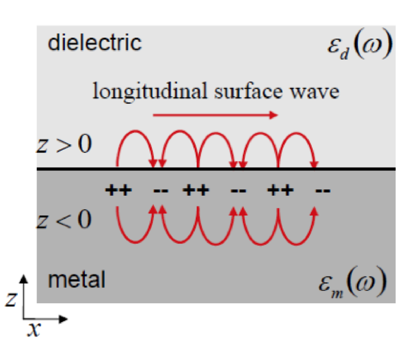
Figure 1: Geometry for SPP propagation at a single interface between metal and dielectric.

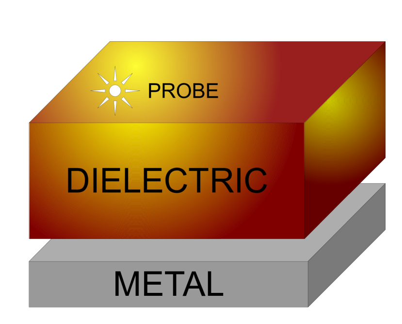
Figure 2: Implemented geometry in COMSOL.

4 The Proposed Neural Network Architecture

The prediction of $\lambda_{SPP}$ and $L_{SPP}$ from the set of values $\lambda_{0}$ and $t$ is related to the problem of the dependence of $L_{SPP}$ from $\lambda_{SPP}$. To obtain a correct prediction of $\lambda_{SPP}$ by a neural network-based approach a value of $\lambda_{SPP}$ is needed. Although this can be obtained by a cascade process, the traditional means have that the NN cascade is accommodated by separate training sessions for each different dedicated NN. Unfortunately, such training sessions would result in very time-consuming computation.

In order to overcome the said complication, this paper proposes a novel parallel paradigm for training that manages to run a single comprehensive training for the NN cascade as a whole, thus avoiding separate training phases. This novel solution has been used for the problem at hand, described in Section 2.

Essentially, the adopted topology has been derived from a pair of common two-layer feed-forward neural networks (FFNNs) [8], used to separately predict $\lambda_{SPP}$ and $L_{SPP}$, respectively. The comprehensive structure is similar to a cascade feed-forward, whereby the output of the first neuroprocessing stage is connected with the input of the second stage and form a new extended input vector for the second stage. On the other hand, the vector provided as input to the second neuroprocessing stage depends on the predicted values obtained from the first stage, hence it propagates a prediction error.

Moreover, during the training phase, while some outputs can be validated for the first neuroprocessing stage, the localised deviation from the correct frequency spectrum could corrupt the training of the second stage. The behaviour of this novel topology is as a two step processing of the data signal that is comprehensive also of a so called second validation or $\omega$-validation, described in the following, aiming at avoiding such an error propagation, which would otherwise endanger the correct training of the second neuroprocessing stage.

A given output from the first stage has to be validated on the frequencies domain, by a validation module, before it can be used. This validation module performs the $\omega$-validation by means of the Fourier computation on a delayed Gaussian window of the output and training signal.

An intermediate level of data processing requires the implementation of a module performing the Fourier transform of the data. Its relative parameters are not a priori established, however are on-line determined by the novel NN topology and then by its training procedure.

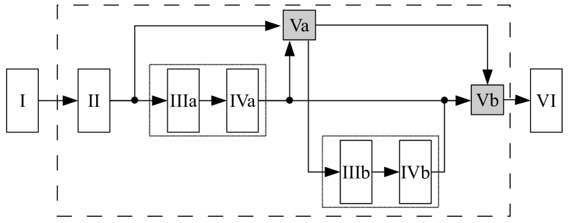
Figure 3: The proposed cascade NN architecture

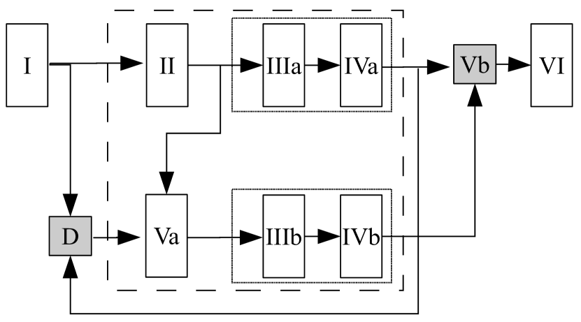
Figure 4: An equivalent recurrent schema

Fig. 4 represents the proposed architecture, which will be detailed in the following. It is possible to recognise two groups of modules, the first comprising IIIa and IVa, whereas the second IIIb and IVb, each acting as a FFNN. The proposed novel topology behaves as a cascade FFNN topology [9]. Fig. 4 depicts a more complex novel topology that performs the prediction as a Nonlinear AutoRecoursive with exogenous inputs (NARX) recurrent neural network topology [10]. Such figure shows the implemented delay lines to the blocks performing the neural processing. It should be noted that we have implemented one neuron as a purelin while the remaining neurons in the first hidden layer process the input signal. The performed simulations have shown an increased computational effort, for this recurrent scheme, while the corresponding results have not significantly improved the accuracy on the predicted data. Even though this is a novel recurrent cascade topology this paper fully investigates the scheme shown in Fig. 4. The following provides the details of the proposed NN cascade.

Input data analysis.

The input layer (I) does not directly provide the input vector ($\mathbf{u}$) to the first FFNN hidden layer (IIIa), being it firstly processed by an intermediate layer (II) that is trained to extrapolate a set of parameters necessary to perform the $\omega$-validation, i.e. the $\sigma$ for the Gaussian window Fourier analysis. This layer (II) is also provided with ad adjunct purelin neuron acting as a transmission line for the following layer (IIIa).

The main purpose of II is to characterise the frequency peaks windows on the data spectrum in order to associate, after the training phase, an optimum $\sigma$ value to perform gaussian-window Fourier analysis on the output data from the second FFNN hidden layer (IVa). For this reason, the input to the following layers are provided as

$$\begin{array}[]{rll}\mathbf{x}^{\texttt{Va}}=&\mathbf{y}^{\texttt{II}}(\mathbf{x}^{\texttt{I}})=&[\tau,\Delta_{\tau},\sigma|\mathbf{x}^{\texttt{I}}]\\ \\ \mathbf{x}^{\texttt{IIIa}}=&\mathbf{x}^{\texttt{I}}&{}\\ \end{array}$$ (10)

where $\mathbf{x}^{\texttt{Va}}$ retains the discrete sample number $\tau$ and both the window size $\Delta_{\tau}$ and $\sigma$ for the described Fourier analysis.

FFNNs hidden layers

The first neuroprocessing module acts as a fully connected FFNN and consists of two hidden layers, i.e. IIIa and IVa. The first hidden layer (IIIa) embeds 10 neurons with tansig activation function, whereas the second hidden layer (IVa) consists of 7 neurons with logsig activation function. Similarly, the second neuroprocessing module provides the functionalities of a fully connected FFNN, however its two hidden layers, IIIb and IVb, consist of 8 and 5 neurons with tansig activation function, respectively.

FFNN training and validation

The implemented FFNN neuroprocessing modules are trained by the Levenberg-Marquardt algorithm with a gradient descent method. Hence, for the $\tau$-esime discrete time step, the variation introduced to the weights are given by

$$\begin{array}[]{rl}w^{\mu\nu}_{ij}(\tau)=&w^{\mu\nu}_{ij}(\tau-1)-\eta e(\tau)\frac{\partial e(\tau)}{\partial w^{\mu\nu}_{ij}(\tau)}\\ \\ e^{\mu}(\tau)=&\tilde{\mathbf{y}}^{\mu}(\tau)-\mathbf{y}^{\mu}(\tau)\end{array}$$ (11)

where $w^{\mu\nu}_{ij}(\tau)$ represents the value for the $\tau$-esime step of the connection weight from the $i$-esime neuron of the $\mu$ layer to the $j$-esime neuron of the $\nu$ layer, $\eta$ is the learning rate parameter, $\tilde{\mathbf{y}}^{\mu}(\tau)$ and $\mathbf{y}^{\mu}(\tau)$ are respectively the training and output signal from the $\mu$ layer.

$\omega$-validation

The output of the first neuroprocessing module comes from the second FFNN hidden layer (IVa) and is sent, as valid output, to the last layer of the network and also as input to the validation module (Va). The validation module consists of a functional unit performing the fast Fourier transform on a selected window of the input signals. Moreover, the validation module uses a dynamically allocated buffer to implement a size-varying delay line.

The latter is used to enable real-time online resizing of the Fourier window to suit the properties of the investigated signal. These adjustments are performed starting from the parameters contained in $\mathbf{x}^{\texttt{Va}}$ (LABEL:eq:io1). Once the gaussian windowed Fourier transform has been computed, the following values are determined

$$\begin{array}[]{rl}M(\tau,\Delta_{\tau},\sigma)=&\max\limits_{[\tau:\tau+\Delta_{\tau}]}\left\{~{}\left|\hat{F}_{\sigma}[\tilde{\mathbf{y}^{\texttt{IVa}}}]-\hat{F}_{\sigma}[\mathbf{y}^{\texttt{IVa}}]\right|~{}\right\}\\ m(\tau,\Delta_{\tau},\sigma)=&\min\limits_{[\tau:\tau+\Delta_{\tau}]}\left\{~{}\left|\hat{F}_{\sigma}[\tilde{\mathbf{y}^{\texttt{IVa}}}]-\hat{F}_{\sigma}[\mathbf{y}^{\texttt{IVa}}]\right|~{}\right\}\end{array}$$ (12)

then the module is trained to admit only certain regions of the $(M,m)$ pairs plan which validate the output signal of the layer IVa.

If the output signal results validated, it is then sent as input for the layer IIIb as

$$\mathbf{x}^{\texttt{IIIb}}=[\mathbf{x}^{\texttt{I}}|\mathbf{y}^{\texttt{IVa}}]$$ (13)

The first neuroprocessing module takes $\mathbf{x}^{\texttt{I}}$ as input and is trained by all the available patterns, while the second module is trained only by the allowed sequences selected according to the validation procedure. In the other case, i.e. if the $\omega$-validation is negative, the second module skips the data during the training process and gives a NaN flagging, being the relative data for the second variable unavailable.

Final output

Finally, the implemented topology gives a global output with a layer consisting of two neurons purelin.

5 Training procedure on OpenMP

The neural network architecture proposed above has introduced a sequential validation phase for the results of the first neuroprocessing module. Validation has to be performed before the first module results can be sent as input for the second module. Unfortunately, such sequential operations make the training process expensive in terms of CPU time. In order to shorten training time, this section describes a parallel implementation of the same neural network architecture, using OpenMP, that manages to obtain asynchronous training and validation.

Generally, when parallelising an application using OpenMP, processes are forked, joined and synchronised (e.g. by means of a barrier). Such mechanisms, however, introduce a runtime overhead, e.g. when the processes having produced and communicated their results have to wait until the synchronisation barrier is over. This is often the case when the computation times of processes are not perfectly balanced [11]. Therefore, our parallel version aims at reducing such an overhead by avoiding, as much as possible, the fork-join-barrier constructs, and by introducing instead processes that produce and consume data. The main reason for using OpenMP is that, by means of a shared memory, communication overhead among processes can be avoided, however, on the other hand, shared memory requires a complex handling of semaphores and locks before accessing some parts of the memory itself. We have handled the synchronisation concern in such a way that overhead is minimised [12].

Mainly, the proposed parallel solution is based on the continuous execution of different processes to care for the different phases of training for the above NN cascade. In our experiments a multi-core processor has been used, however any kind of shared memory system supporting OpenMP directives can be employed.

The proposed NN cascade has been trained to predict the values of $\lambda_{SPP}$ and $L_{SPP}$ starting from an input vector

$$\mathbf{u}(\tau)=\left[\lambda_{0},t\right]$$ (14)

To evaluate the performance of the NN cascade, two different kinds of error were considered. We define two local errors $e^{\texttt{a}}$ and $e^{\texttt{b}}$, as well as a global error $e^{*}$ as follows:

$$\begin{array}[]{rl}e^{\texttt{a}}=&\tilde{\mathbf{y}}^{\texttt{IVa}}-\mathbf{y}^{\texttt{IVa}}\\ e^{\texttt{b}}=&\tilde{\mathbf{y}}^{\texttt{IVb}}-\mathbf{y}^{\texttt{IVb}}\\ e^{*}=&\max\left\{e^{\texttt{a}},e^{\texttt{b}}\right\}\geq\left|\tilde{\mathbf{y}}^{\texttt{VI}}-\mathbf{y}^{\texttt{VI}}\right|\end{array}$$ (15)

where $\tilde{\mathbf{y}}$ indicates the training value.

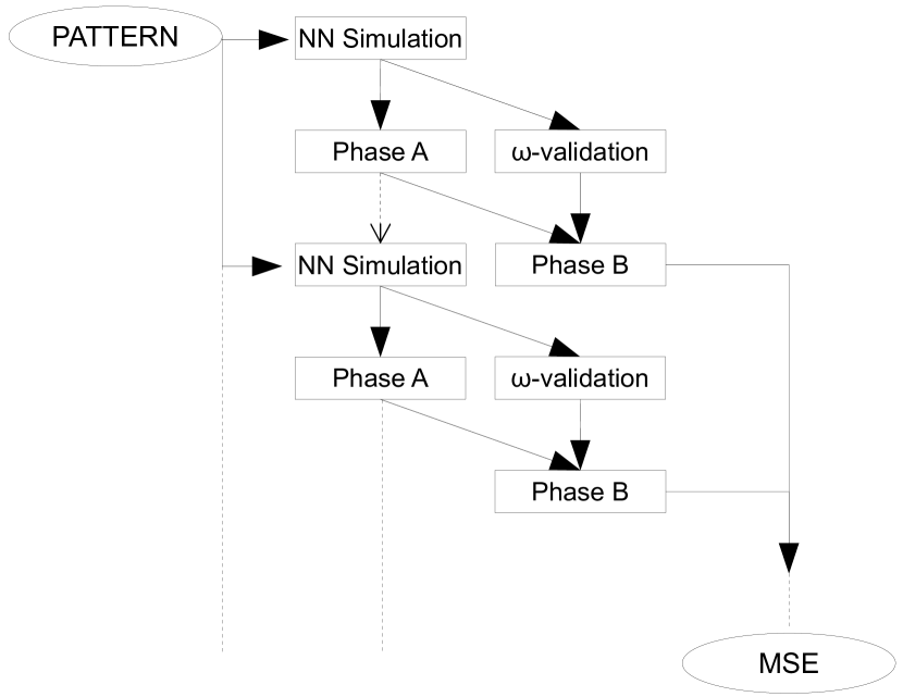
Figure 5: The proposed OpenMP training asynchronous stream

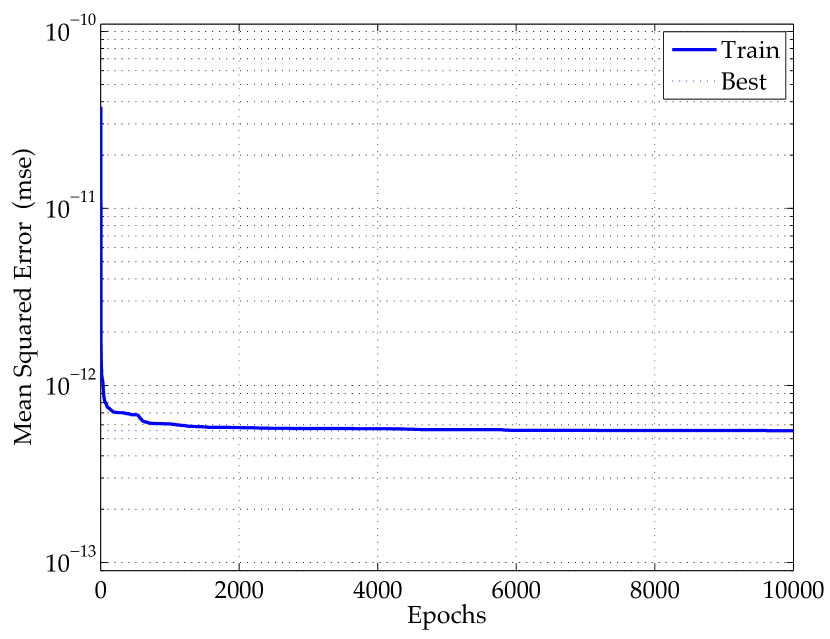
Figure 6: Global performance graph of the implemented NN architecture

For each training epoch, the outputs from layers IVa, IVb and VI (see Fig. 4.) were used to compute the errors $e^{a}$, $e^{b}$ and $e^{*}$ as in (15). The training has been organised in four different activities, executed on an OpenMP environment (see Fig. 6).

The first activity, named NN Simulation, feeds the whole neural network cascade with a training pattern, which has been previously generated.

The second activity, named Phase A, and started once the first activity has terminated, uses a gradient descent algorithm to adjust the neural weights of the intermediate layer II and the first neuroprocessing (layers IIIa and IVa).

The third activity is the $\omega$-validation and is started concurrently with Phase A, hence after NN Simulation has finished, since the results produced by IVa are needed. The $\omega$-validation activity performs the gaussian windowed fast Fourier transform of the training set and the predicted signal resulting as output of IVa, then $M$ and $m$ defined in (12) are computed. Eventually, the values of $M$ and $m$ are used to decide if the pattern data are usable to train the second neuro-processing module (IIIb and IVb).

Finally, the fourth activity is Phase B performing a further training that adjusts the output weights of layer VI. For the proposed schema (see Fig. 4), module Vb acts as a controller determining whether it is appropriate to merge data from IVa and IVb before they can be given as input to VI. The merge is enabled when the $\omega$-validation has given a positive result, otherwise only data resulting from IVa are used. Moreover, all the weights in layer VI are adjusted when the result of $\omega$-validation is positive, otherwise only the synaptic weights of the first neuron in VI is adjusted.

The four activities above are started each as a process (see Fig. 6). Process NN Simulation feeds data and triggers the execution of processes Phase A and $\omega$-validation. The latter two processes give their outputs to process Phase B, and then wait for new data, till the training stops. Process Phase B starts as soon as input data are available. At the end of the training epoch the global network performances are stored for further analysis. All the measures of performance involved in the training process are given by the Mean Squared Error (MSE), though for the global network performances, the formula is adjusted by using the global error $e^{*}$ of (15).

Fig. 6 shows in two vertical tiers some rectangles. Each rectangle corresponds to a process that can execute in parallel with another that is on the same row. In the picture, the time evolves while going down. The arrows with continuous lines represent a flow of data from a producer to a consumer process, whereas the dotted line the communication of an event. Ellipses show repositories of data. The said interactions among processes are iterated until the training session stops.

While having devised a parallel solution, our effort has been to optimise the use of computational resources, hence autonomous processes needing as less synchronisation as possible have been implemented as described above. Our proposed solution manages to greatly reduce the wall-clock timeframe needed for the training.

6 Results and conclusions

For training and evaluation we have used the global error $e^{*}$ to compute the mean square error (MSE) of the network. Fig. 6 shows the performance of the proposed and implemented novel cascade NN architecture in terms of such metrics. Fig. 7 reports the values of the computed and predicted $\lambda_{SPP}$ and $L_{SPP}$. The obtained results confirm the good predictions obtained by the novel NN schema.

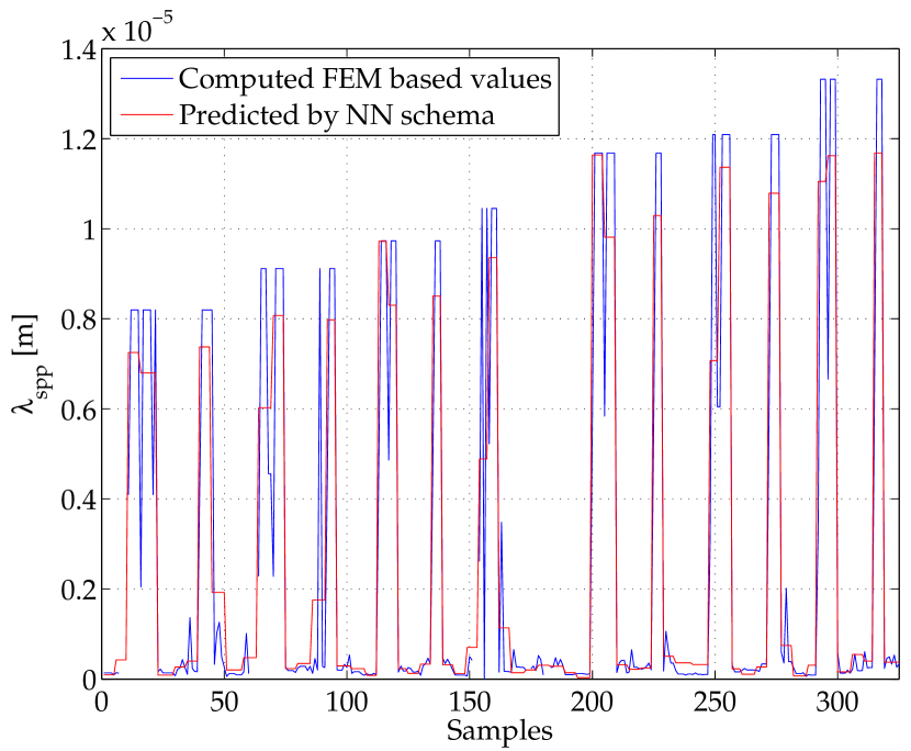
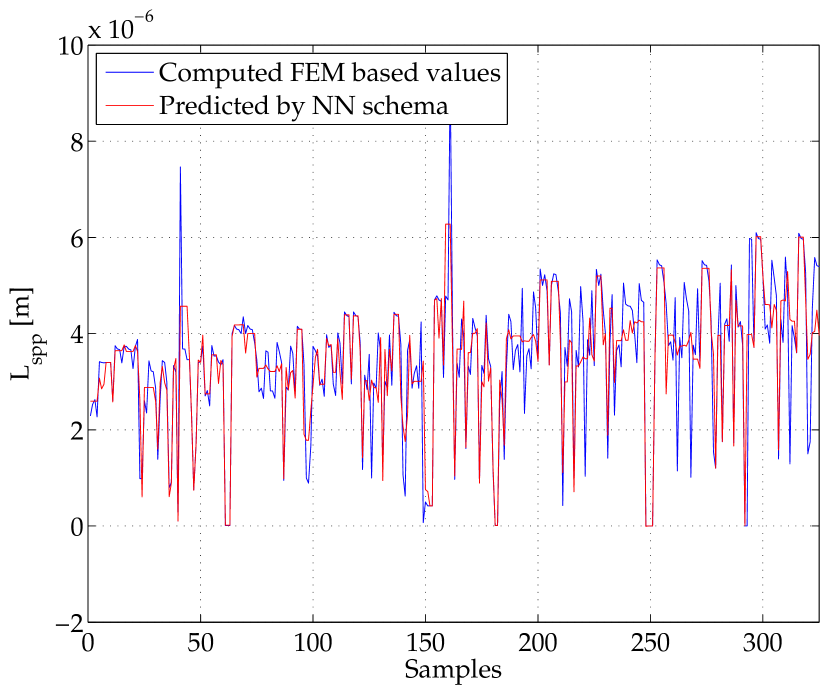
Figure 7: The computed and predicted $\lambda_{SPP}$ and $L_{spp}$

The proposed NN cascade has been mainly derived from a couple of common two-layer feed-forward neural networks used to separately predict $\lambda_{SPP}$ and $L_{SPP}$. The comprehensive structure is similar to a cascade feed-forward, where the output of the first neuroprocessing stage has been connected with the inputs for the second stage to form a new extended input vector.

Simulation results for the NN cascade confirm the effectiveness of the developed novel architecture whose performance during the training and evaluation phases show a very low MSE. Other complex NN architectures such as pure NARX model or advanced Wavelet Recurrent Neural Networks [13] could not be used because of the prediction instability for the data at hand.

References

- [1] Franken, R.H., Stolk, R.L., Li, H., Van der Werf, C. H M., Rath, J.K., Schropp, R. E. I.: Understanding light trapping by light scattering textured back electrodes in thin film n-i-p-type silicon solar cells. Journal of Applied Physics , 102(1), 14503-14509 (2007)
- [2] Atwater, H. A., Polman, A.: Plasmonics for improved photovoltaic devices. Nature Materials, 9(3), 205–213 (2010).
- [3] Fahr, S., Rockstuhl, C., Lederer, F.: Metallic nanoparticles as intermediate reflectors in tandem solar cells. Appl. Phys. Lett., 95(12), 121105-121107 (2009)
- [4] Walters, R. J., van Loon, R. V. A., Brunets, I., Schmitz, J.,Polman, A. : A silicon-based electrical source of surface plasmon polaritons. Nature Materials, 9(3), 21–25 (2010).
- [5] De Waele, R., Burgos, S. P., Polman, A., Atwater, H. A.: Plasmon dispersion in coaxial waveguides from single-cavity optical transmission measurements. Nano Lett. 9, 2832–2837 (2009).
- [6] Shah, A., Torres, P., Tscharner, R., Wyrsch, N., Keppner, H.: Photovoltaic technology: the case for thin-film solar cells. Science 285(5428), 692-698 (1999).
- [7] Maier, S.A.: Plasmonic : Fundamentals and Applications. Springer (2007).
- [8] Mandic, D. P., Chambers, J.: Recurrent neural networks for prediction: learning algorithms, architectures and stability. John Wiley & Sons, Inc., (2001).
- [9] Schetinin, V.: A learning algorithm for evolving cascade neural networks. Neural Processing Letters 17.1, 21-23 (2003).
- [10] Williams, R. J., Zipser, D.: A learning algorithm for continually running fully recurrent neural networks. Neural computation 1.2, 270-280 (1989).
- [11] Dagum, L., Menon, R.: OpenMP: an industry standard API for shared-memory programming. IEEE Computational Science & Engineering, 5.1 46-55 (1998)
- [12] Chapman, B., Jost, G., Van Der Pas, R. : Using OpenMP: portable shared memory parallel programming. Vol. 10. The MIT Press (2008).
- [13] Capizzi, G., Napoli, C., Paternò, L.: An innovative hybrid neuro-wavelet method for reconstruction of missing data in astronomical photometric surveys. International conference on Artificial Intelligence and Soft Computing (ICAISC’12), Vol I, 21-29 (2012).