Quantum Criticality of Topological Phase Transitions in 3D Interacting Electronic Systems
Abstract
Topological phase transitions in condensed matters accompany emerging singularities of the electronic wave function, often manifested by gap-closing points in the momentum space. In conventional topological insulators in three dimensions (3D), the low energy theory near the gap-closing point can be described by relativistic Dirac fermions coupled to the long range Coulomb interaction, hence the quantum critical point of topological phase transitions provides a promising platform to test the novel predictions of quantum electrodynamics. Here we show that a new class of quantum critical phenomena emanates in topological materials breaking either the inversion symmetry or the time-reversal symmetry. At the quantum critical point, the theory is described by the emerging low energy fermions, dubbed the anisotropic Weyl fermions, which show both the relativistic and Newtonian dynamics simultaneously. The interplay between the anisotropic dispersion and the Coulomb interaction brings about a new screening phenomena distinct from the conventional Thomas-Fermi screening in metals and logarithmic screening in Dirac fermions.
Fathoming quantum phases and the associated phase transitions is one of the most significant problems in modern condensed matter physics. Through the natural extension of classical order parameters, the conventional symmetry breaking paradigm has been successfully applied to quantum systems and has deepened our understanding, especially of magnetism and superconductivity.1; 2; 3 On the other hand, the recent theoretical advances in the study of topological orders have provided solid theoretical grounds to predict exotic topological phases. Due to the lack of the classical counterparts, the description of these exotic topological phases and the phase transitions between them is far beyond the realm of the conventional paradigm.4 For instance, through the recent active studies of the systems with strong spin-orbit coupling, a new topological semi-metal (SM), dubbed the Weyl SM, is proposed in systems such as A2Ir2O7 5; 6; 7 or topological insulator multilayers 8. In Weyl SM, composed of several gapless points (Weyl points) on the Fermi energy , the bulk energy spectrum shows the 3D linear dispersion relation around each Weyl point (WP). Contrary to the conventional phases distinguished by order parameters, the Weyl SM is characterized by the topological number, so-called the chirality of WP whose nontrivial topological nature gives rise to the “Fermi arc” surface states. Since the chirality of each WP guarantees its stability, the topological phase transition from the Weyl SM must accompany the pair-annihilation of WPs. 7 In this way, the nature of the Weyl SM and its topological phase transition can be clearly described as long as the interaction between electrons is neglected.
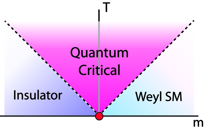
However, the complete understanding of topological phases and related phase transitions in interacting Weyl SM requires the careful consideration of electron correlation effects. For instance, because of the relativistic nature of the electronic dispersion in Weyl SM, the fermionic excitations coupled to the long range Coulomb interaction induce logarithmic corrections to all physical quantities. 9; 10; 11; 12 Moreover, in the presence of the cubic and time reversal symmetries, the interplay between the fermions and the long range Coulomb interaction induces the non-Fermi liquid phase after the pair-annihilation of WPs. 13; 14; 15 In fact, in generic systems without high symmetries, the pair-annihilation of WPs generates insulating phases as shown in Fig. 1. Since the critical point is connected to the insulating phase, the effective theory of the quantum phase transition should respect the zero-chirality condition. Thus, the minimal model for the phase transition is the 3D anisotropic Weyl fermion (AWF) whose dispersion is quadratic along one direction but linear along the other two orthogonal directions. It is worth to note that AWF can emerge ubiquitously in materials breaking either the time-reversal symmetry or the inversion symmetry, and mediate various topological phase transitions. 16; 17; 18 For instance, the recent theoretical 16; 19 and experimental 20 studies on BiTeI have shown that the same critical theory describes the direct topological phase transition between the trivial and topological insulators. Therefore for the universal description of topological quantum phase transitions in generic topological materials, it is crucial to unveil the intriguing quantum criticality of the 3D AWF coupled to the long range Coulomb interaction, which is the main subject in this study.
The main finding of this work is as follows. Most importantly, we find that the anisotropic dispersion of AWF induces exotic screening effects. Namely, significant screening appears along the direction with linear dispersion of electrons in the sense that the momentum dependence of the Coulomb potential is strongly modified from the bare value along that direction. On the other hand, along the direction with quadratic dispersion of electrons, the Coulomb potential is just weakly modified. We call this the anisotropic partial screening phenomenon. Strikingly, such a nontrivial screening effect makes the Coulomb interaction irrelevant in the low energy limit. Thus, the critical theory becomes a non-interacting fermion theory eventually, which allows the complete theoretical understanding of the problem. This behavior is in sharp contrast to the cases of other SMs such as graphene and conventional Weyl SM with isotropic dispersion where the Coulomb potential remains marginal in the infrared limit rendering various physical quantities to receive logarithmic temperature dependence. 9; 10; 11; 12; 23 The nontrivial screening effect of interacting AWF can give rise to intriguing dielectric responses of the system, which will be discussed below.
Model
We begin with the description of the noninteracting AWF. The effective Hamiltonian density has a simple form given by,
| (1) |
where is the velocity for the electron motion in plane and is the inverse of the effective mass along the direction. The Pauli matrices () are used to indicate the conduction and valence bands. Since the system lacks either the inversion symmetry or time reversal symmetry, the gap-closing point is associated with only two bands in general. 16; 17; 18 The topological phase transition from a Weyl SM to an insulator can be described by adding the perturbation term . Depending on the relative sign between and , the ground state becomes either an insulator () or a Weyl SM () with a pair of WPs having opposite chiralities. 17; 18 At the quantum critical point , the two WPs pair-annihilate at a certain momentum point at which the net chirality should obviously be zero. Such a zero chirality condition forces the electron dispersion to be nonlinear at least along one direction, which leads to the minimal Hamiltonian for the AWF as shown in (1). In general, the quadratic dispersion occurs along the direction in which a pair of WPs migrate before they are pair-annihilated. 17; 18 We provide a simple lattice model which captures all essential characteristics of the topological phase transition between the Weyl SM and an insulator in Supplementary Note 1.
To describe the dynamics of AWF coupled to the long range Coulomb interaction, we use the Euclidean path integral formalism and write the effective action as follows.
As usual, the momentum cutoff () is implicitly assumed. The matrices , satisfying , are defined as ,,. () represents an electron (boson) field operator and . The Hubbard-Stratonovich transformation introduces the bosonic field for the instantaneous Coulomb interaction. The dimensionless parameter is used to capture the possible anisotropy of the Coulomb potential induced by the anisotropic fermion dispersion. The electrons are coupled to the boson via the coupling constant where is the electric charge and is the dielectric constant.
Considering the anisotropic dispersion of electrons, the coupling constants in the action naturally lead to three characteristic energy scales, , , and which describe the electron kinetic energy () and Coulomb potential () and the cutoff energy () related with the linear dispersion of electrons, respectively. The associated dimensionless coupling constants are
| (2) |
Although only two of them are independent (), for notational convenience, we use the three coupling constants to perform the renormalization group (RG) analysis.
The anisotropic fermion dispersion gives rise to unusual scaling properties of the system. Let us first consider the noninteracting fermions with the following scale transformation
| (3) |
where the rescaled variable is indicated by a tilde. Namely, the scaling dimension of , , and are given by , , . It is worth to note that since the dispersion of the fermion is anisotropic while that of the boson is isotropic, the scale invariance of the whole system requires to introduce the general scaling dimension . However, our RG results (below) are independent of as it should be. The invariance of the fermionic part of the action under the scale transformation in (3) leads to the following scaling relations at the tree level, , . If we assume that is marginal while is either marginal or irrelevant, we obtain , and . On the other hand, if is marginal while is either marginal or irrelevant, , , and . Therefore the Coulomb interaction is marginal for while it is irrelevant otherwise, hence we focus on the case of in the following.
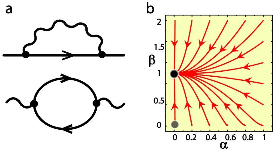
Renormalization group analysis.- We perform a momentum shell RG analysis of at one-loop level. Because of the anisotropic dispersion, it is natural to consider two different momentum cutoffs, i.e., for the dispersion in the plane of and for the dispersion. For convenience, we set and perform the momentum-shell integration in the following way, where and . In principle, three Feynmann diagrams need to be considered for the RG calculation at one-loop order, i.e., the fermion self-energy, the boson self-energy and the vertex correction. Since the fermion self-energy is frequency independent for the instantaneous bare Coulomb interaction, the vertex correction vanishes, consistent with the Ward identity in one-loop calculation. Therefore, the two Feynman diagrams shown in Fig. 2a determine the RG flow.
The RG flows of the three coupling constants , , describe quantum corrections from the interaction. Instead of showing the details, we only present the beta functions leaving technical calculations to the Supplementary Note 2.
| (4) |
Note that and are absent in (4) as expected. The RG flow is illustrated in Fig. 2b which shows two fixed points at () = (0,0) and () = (0,1), respectively. At both fixed points, . The flow emerges from the former (unstable) fixed point and terminates at the latter (stable) one. Interestingly, the fine-structure constant () is zero at both fixed points. The linear dependence of the electron self-energy,
| (5) |
manifestly shows that the electrons basically become free from interaction in the low energy limit.
The distinct natures of the two fixed points are clearly revealed in the screening effect of the Coulomb potential. The inverse of the boson propagator including the self-energy correction () becomes,
Here the unimportant dependence is neglected. At the unstable fixed point, , the Coulomb potential decouples from electrons. On the other hand, at the stable fixed point, , the Coulomb potential receives a nontrivial correction in the direction while there is no screening in the direction. The non-trivial correction can be understood as the strong screening effect with the anomalous dimension. Considering the different scaling between the and directions, we obtain
at the stable fixed point. Thus, the Coulomb potential receives anisotropic partial screening through the interaction with electrons. Here can be fixed from the condition that and do not run at the stable fixed point. Then, the momentum anisotropy gives at the stable fixed point. Therefore the renormalized Coulomb interaction has the following structure at the fixed point. It means that in the real space depends on the spatial coordinate anisotropically as and .
Screening of a charged impurity
The novel quantum effect in interacting AWF can induce unusual dielectric responses of the system. Here we consider the screening problem of a Coulomb impurity with the electric charge () by AWF. Because of the non-trivial quantum corrections caused by interacting fermions, the distribution of the screening charge in interacting AWF can be completely different from that in the non-interacting system. Let us first consider the noninteracting AWF coupled to a single charged impurity, which can be described by the following Hamiltonian,
| (6) |
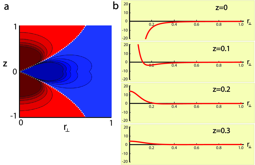
where is the coupling constant of the noninteracting system. In fact, because of the anisotropic momentum dependence of the polarization function which can be summarized as with the positive constants and , the screening charges distribute in a highly unusual way even in the noninteracting system. According to the linear response theory, the induced charge density is given by where . 21 As shown in Fig. 3, the peculiar structure of gives rise to strong spatial anisotropy in the distribution of the induced charges in real space, . In particular, owing to the anisotropy of , the partially integrated charge densities and show characteristic coordinate dependence such as
where in which indicates the Bessel function of the first kind. Here is defined as with the in-plane momentum cutoff . This sharp momentum cutoff causes the oscillation of with fixed amplitude. Notice that the partially integrated charge densities distribute in a highly unusual way, i.e., is strongly localized near the impurity while shows slow decay with a power-law tail. The detailed behavior of is shown in Supplementary Note 3.
Surprisingly, the strong Coulomb interaction between electrons completely modify the screening charge distribution in AWF. Since all coupling constants are irrelevant at the stable fixed point, the induced charge can be computed to the leading order by using and . Since the amount of the total induced charge is fixed, i.e., , is fixed to be , which gives rise to . In contrast to the case of the noninteracting system, the screening charge is strictly localized near the impurity site. Similar localized distribution of the induced charge is predicted in graphene. 22 In graphene, it is shown that the Coulomb interaction can induce small spreading of the screening charge in subleading order. However, in our case such an additional spreading of the screening charge can only play a minor role since the Coulomb interaction is irrelevant at the fixed point while it is marginal in graphene. 23; 24
Discussion
Up to now we have considered the system having a single AWF. However, in real materials, several AWFs can simultaneously appear at the Fermi level due to the time-reversal or crystalline symmetries. In this case, to describe the renormalized Coulomb interaction, it is necessary to add the contribution from all AWFs to the polarization. In other words, the polarization function should be given by where indicates the polarization due to the th AWF. Here it is assumed that the polarization induced by the coupling between neighboring AWFs can be neglected, which is valid if the distance between AWFs is far enough. The important point is that the direction along which the AWF shows the quadratic dispersion can vary for different AWFs in general. Therefore in the system with multiple AWFs, the total polarization should behave as on average with . In this case, the renormalized Coulomb interaction should have the following form of . Equivalently, it means that the long range Coulomb interaction shows the unusual power law given by in real space due to the screening effect. If we introduce a charged impurity to this system, the induced charge spreads in a way of when the electron-electron interaction is neglected. On the other hand, once the electron-electron interaction is considered, the induced charge is again strictly localized near the impurity site, i.e., with a constant .
The results from our perturbative RG approach are further supported by the random phase approximation (RPA) approach. As shown in the Supplementary Note 4, we find that along the direction with linear (quadratic) dispersion, the momentum dependence of the polarization shows (). Note that the RPA and the one-loop RG calculations match perfectly, thus we believe that the results of the one-loop RG calculation is robust. Besides the fact that two different methods give the same momentum dependence of , we further consider the corrections to the RPA results by performing the strong coupling expansion. As shown in Supplementary Note 5, it is explicitly proved that the quantum fluctuations near the stable fixed point do not cause any divergent corrections confirming the robustness of the conclusions obtained from the RG analysis.
To conclude, we have rigorously demonstrated the novel quantum critical phenomena of the AWF. We emphasize that the anisotropic partial screening is clearly distinct from the conventional screening phenomena in usual metallic or semi-metallic systems, which is concisely summarized in Table 1. For example, the Thomas Fermi screening in conventional metals forces the renormalized Coulomb interaction to be short-ranged and the fermionic excitations coupled by the short range repulsive interaction gives rise to the Fermi liquid state. 25 On the other hand, in the AWF, the interplay between the Coulomb interaction and fermions induces the anisotropic partial screening, which allows the screened Coulomb interaction to maintain the long-ranged nature and the fermions to be free from the Coulomb interaction in the low energy limit. Therefore the anisotropic partial screening can be considered as the intermediate screening phenomena distinguished from both the Thomas-Fermi screening in metals and the logarithmic screening in Dirac fermions, which is uncovered for the first time in this study.
References
- (1) Sachdev, S., Quantum Phase Transitions. Cambridge University Press. (2nd ed.) (1999).
- (2) Balents, L., Spin liquids in frustrated magnets. Nature 464, 199-208 (2010).
- (3) Xu, C. Unconventional quantum critical points. Int. J. Mod. Phys. B 26, 1230007 (2012).
- (4) Wen, X. G. Topological Order: From Long-Range Entangled Quantum Matter to a Unified Origin of Light and Electrons. ISRN Condensed Matter Physics 2013, 198710 (2013).
- (5) Wan, X., Turner, A. M., Vishwanath, A., & Savrasov, S. Y., Topological Semimetal and Fermi-Arc Surface States in the Electronic Structure of Pyrochlore Iridates. Phys. Rev. B 83, 205101 (2011).
- (6) Ueda, K.,Fujioka, J.,Takahashi, Y., Suzuki, T.,Ishiwata, S.,Taguchi, Y., & Tokura, Y., Variation of Charge Dynamics in the Course of Metal-Insulator Transition for Pyrochlore Type Nd2Ir2O7. Phys. Rev. Lett 109, 136402 (2012).
- (7) Balents, L., Viewpoint: Weyl electrons kiss. Physics 4, 36 (2011).
- (8) Burkov, A. A.& Balents, L., Weyl Semimetal in a Topological Insulator Multilayer. Phys. Rev. Lett 107, 127205 (2011).
- (9) Hosur, P.,Parameswaran, S. A.,& Vishwanath, A., Charge Transport in Weyl Semimetals. Phys. Rev. Lett 108, 046602 (2012).
- (10) Isobe, H.,& Nagaosa, N., Theory of a quantum critical phenomenon in a topological insulator: (3+1)-dimensional quantum electrodynamics in solids. Phys. Rev. B 86, 165127 (2012).
- (11) Isobe, H.,& Nagaosa, N., Renormalization group study of electromagnetic interaction in multi-Dirac-node systems. Phys. Rev. B 87, 205138 (2013).
- (12) Goswami, P.,& Chakravarty, S., Quantum Criticality between Topological and Band Insulators in 3+1 Dimensions. Phys. Rev. Lett 107, 196803 (2011).
- (13) Luttinger, J. M., Quantum Theory of Cyclotron Resonance in Semiconductors: General Theory. Phys. Rev. 102, 1030 (1956).
- (14) Murakami, S.,Nagaosa, N.,& Zhang, S. -C. SU(2) non-Abelian holonomy and dissipationless spin current in semiconductors. Phys. Rev. B 69, 235206 (2004).
- (15) Moon, E. -G.,Xu, C.,Kim, Y. B.,, & Balents, L., Non-Fermi-Liquid and Topological States with Strong Spin-Orbit Coupling. Phys. Rev. Lett. 111, 206401 (2013).
- (16) Yang, B. -J., Bahramy, M. S.,Arita, R. , Isobe, H. ,Moon, E. -G., & Nagaosa, N., Theory of Topological Quantum Phase Transitions in 3D Noncentrosymmetric Systems. Phys. Rev. Lett. 110, 086402 (2013).
- (17) Murakami, S.,& Kuga, S. -i. Universal phase diagrams for the quantum spin Hall systems. Phys. Rev. B 78, 165313 (2008).
- (18) Murakami, S., Phase transition between the quantum spin Hall and insulator phases in 3D: emergence of a topological gapless phase . New J. Phys. 9, 356 (2007).
- (19) Bahramy, M. S.,Yang, B. -J., Arita, R., & Nagaosa, N., Emergence of non-centrosymmetric topological insulating phase in BiTeI under pressure. Nat. Commun. 3, 679 (2012).
- (20) Xi, X., Ma, C.,Liu, Z., Chen, Z. ,Ku, W., Berger, H. ,Martin, C.,Tanner, D. B., & Carr, G. L., Signatures of a Pressure-Induced Topological Quantum Phase Transition in BiTeI. Phys. Rev. Lett. 111, 155701 (2013).
- (21) Kotov, V. N.,Pereira, V. M.,&Uchoa, B., Polarization charge distribution in gapped graphene: Perturbation theory and exact diagonalization analysis. Phys. Rev. B 78, 075433 (2008).
- (22) Kotov, V. N.,Uchoa, B.,Pereira, V. M., Guinea, F.,&Castro Neto, A. H., Electron-Electron Interactions in Graphene: Current Status and Perspectives. Rev. Mod. Phys. 84, 1067 (2012).
- (23) Son, D. T., Quantum critical point in graphene approached in the limit of infinitely strong Coulomb interaction. Phys. Rev. B 75, 235423 (2007).
- (24) Biswas, R. R.,Sachdev, S.,&Son, D. T., Coulomb impurity in graphene. Phys. Rev. B 76, 205122 (2007).
- (25) Shankar, R., Renormalization-group approach to interacting fermions. Rev. Mod. Phys. 66, 129 (1994).
- (26) Yang, K. -Y.,Lu, Y. M.,& Ran, Y., Quantum Hall effects in a Weyl semimetal: Possible application in pyrochlore iridates. Phys. Rev. B 84, 075129 (2011).
Acknowledgements
We are grateful for support from the Japan Society for the Promotion of Science (JSPS) through the ‘Funding Program for World-Leading Innovative R&D on Science and Technology (FIRST Program), and Grant-in-Aids for Scientific Research (No. 24224009) from the Ministry of Education, Culture, Sports, Science and Technology (MEXT). B.-J. Yang and N. Nagaosa greatly appreciate the stimulating discussions with Ammon Aharony, Ora Entin-Wohlman, Michael Hermele, and Miguel A. Cazalilla. E.-G. Moon is grateful for invaluable discussion with Leon Balnets, Max Metlitski, and Cenke Xu and supported by the MRSEC Program of the National Science Foundation under Award No. DMR 1121053.
| Fermionic Excitations | |||
|---|---|---|---|
| Metal | Marginal | Fermi Liquid | |
| Anisotropic Weyl fermion (AWF) | Irrelevant | Fermi Liquid | |
| Weyl SM | Marginally Irrelevant | (Marginal) Fermi Liquid |
Table 1: Physical properties of interacting metallic or semi-metallic systems in 3D coupled with the instantaneous Coulomb interaction. Here “Metal” indicates the conventional metal with Fermi surface and “Weyl SM” means the 3D semi-metal with linear dispersion in all spatial directions. () indicates the screened Coulomb potential (renormalized coupling constant) at the stable fixed point. As for the q dependence of , and indicates the Thomas Fermi screening length. When the electron dispersion is quadratic in all directions, it is shown that the screened Coulomb potential becomes and a non-Fermi liquid ground state can be realized. (Ref. [15])
Supplementary Note 1
Lattice model for anisotropic Weyl fermion.
Here we provide a simple lattice model Hamiltonian describing the topological phase transition from a Weyl SM to an insulator. (See also Ref.[26].) The AWF appears at the quantum critical point. We consider spinless fermions on a tetragonal lattice with two orbital degrees of freedom in the unit cell, which can be represented by
| (7) |
where are the Pauli matrices indicating two orbital degrees of freedom and , are the hopping integrals along the , directions, respectively. Here we assume for convenience. In this system, when , the Weyl SM appears as the ground state which has a pair of Weyl points with opposite chirality along the axis. The critical point at () mediates the quantum phase transition from the Weyl SM to a trivial band insulator (a 3D quantum Hall insulator) which exists for (). At these two quantum critical points, the bulk energy spectrum shows the quadratic dispersion along the direction while it is linear along the plane, which indicates the emergence of the AWF.
Supplementary Note 2
Renormalization Group analysis.
In this section, we provide a detailed description of the RG analysis. To perform the one-loop renormalization group analysis, we write the Euclidean effective action describing the low energy electrons coupled to long range Coulomb interaction in the following way,
which is basically the same as the action in the main text of the paper. Here the instantaneous Coulomb interaction term is decoupled by introducing the bosonic Hubbard-Stratonovich field . The non-interacting electron and boson Green’s functions are given by
where .
Boson selfenergy.- At first we compute the one-loop boson self-energy , which is given by
| (8) | |||||
where . Here indicates the integral over the momentum shell. To determine the renormalization of the bare boson propagator by , we expand in powers of up to quadratic order, which leads to
| (9) |
After a straightforward calculation of the momentum-shell integral, we can obtain
| (10) |
in which
| (11) |
Electron selfenergy.- Now let us consider the renormalization of and by computing the electron self-energy . At one-loop order, can be written as
which, for small and , can be written as
Here are as follows,
where is the usual RG scale parameter and . If we solve the full coupled RG equation, it can be shown that . Therefore we can make an expansion in powers of and the leading contribution to can be written as
| (12) |
The other integrals appearing in can be done in the following way,
| (13) | |||||
Similarly,
Then can be written as
| (14) |
() describes the renormalization of (). Explicitly, for small limit, are given by
| (15) |
RG equations.- Including and , the full effective action can be written as
| (16) | |||||
The one loop RG equations can be obtained in the following way. At first, we rescale the space-time coordinates,
| (17) |
where the tilde is used to indicate the scaled variable. Then we introduce renormalization constants , , , , , and in the following way,
| (18) |
Then we assume that the renormalized action has the same form as the bare action , which leads to
At this point, let us explain the physical meaning of dimensionless variables and . Here indicates the strength of the Coulomb interaction relative to the kinetic energy originating from the linear dispersion. compares the kinetic energy from the quadratic dispersion relative to the kinetic energy coming from the linear dispersion. In terms of and , can be written in the following way.
| (19) |
In the small limit the above RG equations reduce to
| (20) |
Similarly, the RG equations for and can be written as
| (21) | |||||
The RG equations can be neatly expressed by using , , which are defined as
| (22) |
where . Here and can be rewritten in terms of and as follows,
| (23) |
The RG equations for , , are shown in the main text.
Supplementary Note 3
The distribution of the induced charge.
Here we show the detailed structure of the induced charge . After a straightforward computation of the momentum integration, we can obtain the following result.
| (24) |
in which
where . Here K (E) indicates the complete elliptic integral of the 1st (2nd) kind.
When , we can obtain that
On the other hand, when ,
Therefore we can clearly see that and have the opposite sign, which is consistent with the charge distribution shown in Fig. 3a.
Supplementary Note 4
Screened Coulomb interaction in RPA analysis.
To confirm the anomalous structure of the effective Coulomb interaction at the stable fixed point, here we compute the polarization function in the following way.
In contrast to the case of the RG approach where the integration is performed on the momentum shell, we perform the momentum integration over the full range of q and extract the dependence of .
After the integration over , the static polarization can be written as
where . To perform the integration over , we have used the following formula of dimensional regularization
At first, let us consider the case of . A straightforward calculation shows that
Since the above integration is divergent, we introduce a UV cutoff for variable. Then the resulting expression is given by
which shows that the leading dependence is still given by . Similarly, we consider the case of , which is given by
Therefore dependence of the polarization function can be obtained consistent with the result of RG analysis.
Supplementary Note 5
Strong Coupling analysis.
In this section, let us understand the stability of the stable fixed point with the strong coupling analysis. The strong coupling analysis starts with the following action,
omitting unimportant dimensionful numbers. The strong coupling analysis can be verified by the large analysis introducing copies of different fermions. Here instead of evaluating the exact () result, we use the simplified RPA results which capture the correct functional dependence. Since we are only interested in how the infra-red divergence appears, the RPA result is enough to estimate. One parameter () is introduced for comparison, and the discussed anisotropic partial screening corresponds to .
Given the approximated action, we can evaluate correction. The electron self energy with the momentum cutoff () in the quadratic direction is
where and . It is easy to show that the correction from the self-energy is not diverging in the infra-red cutoff,
for . It is manifest that one can set . The absence of the infra-red divergence indicates the irrelevance of the coulomb interaction.
One can further investigate the anisotropic fermion in two spatial dimensions. Following the same method, one can show the linear direction is renormalized significantly, so the strong coupling action becomes
where . Then, the correction from the fermion self energy is
Thus, the anisotropic screening induces the logarithmic correction similar to conventional graphene physics.