MAGNETIC PAIR CREATION TRANSPARENCY IN GAMMA-RAY PULSARS

Abstract

Magnetic pair creation, $\,\gamma\to e^{+}e^{-}\,$, has been at the core of radio pulsar paradigms and central to polar cap models of gamma-ray pulsars for over three decades. The Fermi gamma-ray pulsar population now exceeds 140 sources and has defined an important part of Fermi’s science legacy, providing rich information for the interpretation of young energetic pulsars and old millisecond pulsars. Among the population characteristics well established is the common occurrence of exponential turnovers in their spectra in the 1–10 GeV range. These turnovers are too gradual to arise from magnetic pair creation in the strong magnetic fields of pulsar inner magnetospheres. By demanding insignificant photon attenuation precipitated by such single-photon pair creation, the energies of these turnovers for Fermi pulsars can be used to compute lower bounds for the typical altitude of GeV band emission. This paper explores such pair transparency constraints below the turnover energy, and updates earlier altitude bound determinations of that have been deployed in various Fermi pulsar papers. For low altitude emission locales, general relativistic influences are found to be important, increasing cumulative opacity, shortening the photon attenuation lengths, and also reducing the maximum energy that permits escape of photons from a neutron star magnetosphere. Rotational aberration influences are also explored, and are found to be small at low altitudes, except near the magnetic pole. The analysis presented in this paper clearly demonstrates that including near-threshold physics in the pair creation rate is essential to deriving accurate attenuation lengths and escape energies. The altitude bounds are typically in the range of 2-7 stellar radii for the young Fermi pulsar population, and provide key information on the emission altitude in radio quiet pulsars that do not possess double-peaked pulse profiles. The bound for the Crab pulsar is at a much higher altitude, with the putative detection by MAGIC out to 350–400 GeV implying a lower bound of 310km to the emission region, i.e., approximately 20% of the light cylinder radius. These results are also extended to the super-critical field domain, where it is found that emission in magnetars originating below around 10 stellar radii will not appear in the Fermi-LAT band.

1. INTRODUCTION

The Fermi Gamma-ray Space Telescope has revolutionized our understanding of high-energy emission from pulsars. Prior to the launch of Fermi, there were only 7 high-confidence detections (Thompson et al., 1997) of gamma-ray pulsars from the EGRET telescope aboard the Compton Gamma-ray Observatory (CGRO), of which all but Geminga had a radio counterpart. Except for Geminga, which is extremely bright, EGRET was not sensitive enough to perform blind searches, the process of discerning pulsation in pulsars using their gamma-ray data alone, i.e. without the guide of an existing radio ephemeris. Furthermore, the maximum observed photon energy, typically in the range 1–10 GeV, was just outside the upper end of EGRET’s sensitive energy range. With the launch of Fermi, a wealth of new data became available. In just five years, the gamma-ray pulsar sample increased from 7 to over 120 pulsars (Abdo et al., 2013, lists 117 in the second Fermi-LAT pulsar catalog), including over three dozen millisecond pulsars and over 35 pulsars discovered in Fermi blind searches (Abdo et al., 2009a, 2010a; Saz Parkinson et al., 2010; Abdo et al., 2013). The overwhelming majority of these blind search pulsars have been shown to have no discernible radio counterparts, with upper limits to fluxes at the $\,30\mu\,$Jy level (Abdo et al., 2013). Fermi’s increased sensitivity allows the detection of fainter pulsars, and this combined with better time resolution has given us more detailed pulse shapes than EGRET could provide. The energy window centered on a few GeV is now easily observable for the first time. This has yielded clear observations of spectral cutoffs and determinations of their shapes in the vast majority of pulsars of all classes: old millisecond ones, young radio-quiet and young radio-loud rotators. Such revelations have made it possible to resolve some long-standing questions about the origins of pulsar high-energy emission.

Prior to the launch of Fermi, there were two competing predictions for the shape of the pulsar spectral cutoff. Outer gap models, driven by curvature radiation physics, predicted a simple exponential cutoff (see, for example, Chiang & Romani, 1994), corresponding to the emission by electrons possessing a maximum Lorentz factor. A similar picture exists for slot gap models (Muslimov & Harding, 2004) that extend polar cap-driven emission to high altitudes. In contrast, polar cap models (Daugherty & Harding, 1996) based on low altitude photon emission, magnetic pair creation $\,\gamma\to e^{+}e^{-}\,$ and pair cascading predict a super-exponential cutoff due to the very strong dependence of the pair production rate on photon energy. EGRET data were equally consistent with either cutoff scenario (Razzano & Harding, 2007). With far greater statistics, early Fermi-LAT observations of the Vela pulsar clearly exhibited a simple exponential cutoff (Abdo et al., 2009b), and subsequent observations of Vela and other pulsars have corroborated this shape, demonstrating that exponential cutoffs are present in the phase-resolved spectroscopic data (Abdo et al., 2010b). Super-exponential spectral turnovers in Fermi GeV band data can be ruled out to high degrees of significance. This fact can be used to place a physical lower bound on the altitude of origin for the high-energy emission. The magnetic pair creation process is strongly height-dependent and should dominate at low altitudes. Since the signature of strong pair creation - a super-exponential cutoff in the spectrum - is not observed, the emission altitude must be high enough that attenuation due to single-photon pair production is not expected.

Even though magnetic pair creation-driven cutoffs do not occur in the Fermi pulsar sample, performing calculations of magnetic pair production transparency is still a worthwhile exercise. The associated physical lower bounds for the emission height should be considered as a complement to geometric determinations of the emission height from gamma-ray and gamma-ray/radio peak separation in caustic scenarios (Watters et al., 2009; Pierbattista et al., 2010; Venter, Johnson & Harding, 2012). In particular, magnetic pair creation altitude bounds can help constrain magnetospheric geometry in pulsars that do not possess two distinct gamma-ray peaks (about 30% of the blind search pulsars: Saz Parkinson et al., 2010) and are radio quiet; such pulsars are not as easily amenable to altitude diagnostics using caustic geometry analysis. Furthermore, pair production rates stemming from opacity computations are important for the understanding of pulsar wind nebula energetics. The Goldreich-Julian currents alone cannot carry enough energy to account for PWN luminosities (Rees & Gunn, 1974; de Jager, 2007; Bucciantini, Arons & Amato, 2011), and to achieve the required energy deposition, there must be prolific pair creation occurring in the pulsar magnetosphere. Single-photon magnetic pair creation is very efficient at low altitudes and can produce large pair multiplicities (Daugherty & Harding, 1982; Muslimov & Harding, 2003) approaching, but still somewhat lower than, those needed to achieve the required nebular energy deposition.

Pair opacity calculations date from early pulsar theory, such as in the work of Arons & Scharlemann (1979). Ho, Epstein, & Fenimore (1990), working on early gamma-ray burst theory, recognized that $\gamma-B$ attenuation posed a major problem for the escape of gamma-rays from the neutron star surface. Their calculations, which ignored general relativistic (GR) and aberration effects, showed that for the escape probability to be significant at soft gamma-ray energies, emission must be strongly collimated around the local magnetic field. For the higher-energy gamma-rays seen by Fermi, relativistic beaming guarantees that photons will be emitted essentially parallel to the local magnetic field. In Harding, Baring & Gonthier (1997), although the focus was on photon splitting, the authors carried out single-photon pair production attenuation calculations for comparison purposes. These calculations included detailed consideration of threshold effects in the computation of photon attenuation lengths and escape energies, the latter defining the critical energies above which the magnetosphere is opaque to photon passage for a given emission locale. In an extension of this analysis, Baring & Harding (2001) illustrated the character of magnetic pair creation and photon splitting opacities by exploring the dependence of photon escape energy on the colatitude of emission for each process, for photons originating at the neutron star surface. They also discussed cascading and the conditions under which pair creation (and therefore, arguably, radio emission) should be effectively quenched. Most recently, Lee et al. (2010) tackled the problem of $\gamma-B$ attenuation in detail. Their work, which produced lower bounds for emission altitudes as a function of photon energy, incorporated potentially critical aberration and GR corrections, but largely ignored the threshold behavior of the $\,\gamma\to e^{+}e^{-}\,$ rate.

The physics that determines the form of the $\gamma-B$ attenuation coefficient is discussed in some detail in Section 2. An early offering that described this first-order QED process in a manageable form was in the seminal work by Erber (1966), which provided a simple asymptotic form of the attenuation coefficient. Tsai & Erber (1974) subsequently dealt in detail with the differences in photon polarization modes. Near the pair creation threshold, the simple asymptotic approximations obtained in these works become less accurate, differing on average by over two orders of magnitude from exact pair production rates in fields below around 4 TeraGauss. Daugherty & Harding (1983) provided an empirical approximation to threshold behavior, while formally precise forms were offered in the works of Baring (1988) and Baier & Katkov (2007); none of these is quite as simple as the form highlighted in Erber (1966). These threshold corrections are important to address in pair opacity computations involving regions near the stellar surface, when the local field is near-critical or higher, i.e. especially for magnetars.

In this work, we have taken an analytical approach to the problem of pair creation opacity whenever possible. We present magnetic pair creation transparency conditions as a function of colatitude and height of emission for photons emitted parallel to the local magnetic field, as is approximately the case for curvature emission. Our integrals for the magnetic pair creation optical depth are computed for a variety of photon energies and surface polar magnetic fields $\,B_{p}\,$. We have included, analytically where possible, corrections for threshold conditions on magnetic pair creation, gravitational redshift, general relativistic magnetic field distortion, and aberration due to neutron star rotation. In Section 3 it is found that in flat spacetime, the maximum energy $\,\varepsilon_{\rm esc}\,$ of a photon that can escape the magnetosphere is a declining function of the emission colatitude $\,\theta_{\hbox{\sixrm E}}\,$ and the field $\,B_{p}\,$. In particular, for $\,B_{p}<4\times 10^{12}\,$Gauss, the relationship $\,\varepsilon_{\rm esc}B_{p}\sin\theta_{\hbox{\sixrm E}}\sim\,$ constant    is borne out, in agreement with Arons & Scharlemann (1979) and Chang, Chen, & Ho (1996), a direct consequence of the asymptotic form (Erber, 1966) of the pair production rate. When the surface polar field exceeds around $\,B_{p}\sim 10^{13}\,$Gauss, the threshold influences become profound, and the dependence of $\,\varepsilon_{\rm esc}\,$ on $\,B_{p}\,$ weakens substantially. If one fixes the escape energy, the altitude at which a photon can be emitted and emerge from the magnetosphere unscathed by magnetic pair attenuation is a monotonically increasing function of colatitude $\,\theta_{\hbox{\sixrm E}}\,$.

Including general relativity effects (see Section 4) reduces the attenuation length for pair creation, lowers the escape energies for surface emission locales by 20–30% for $\,B_{p}<4\times 10^{12}\,$Gauss (and around a factor of two for $\,B_{p}\sim 4\times 10^{13}\,$Gauss) and raises the minimum altitudes of emission by at most 10–20%. For emission points above two stellar radii, GR influences are generally insignificant. Including aberration effects (see Section 5) dramatically raises the minimum altitudes $\,r_{\rm min}\,$ for pair transparency at small colatitudes above the magnetic pole. For most emission azimuthal angles, the minimum altitude of emission increases monotonically with colatitude. In addition, $\,r_{\rm min}\,$ quickly maps over to the flat spacetime, non-rotating magnetosphere results when $\,\theta_{\hbox{\sixrm E}}\gtrsim 10^{\circ}\,$ — then aberration influences are largely minimal in the inner magnetosphere because the co-rotation speeds are far inferior to $\,c\,$. This monotonic trend for $\,r_{\rm min}\,$ continues right up to above the magnetic equator, because of the relative ease with which photons cross field lines when propagating at high magnetic colatitudes. In particular, we do not reproduce the putative decline of $\,r_{\rm min}\,$ as $\,\theta_{\hbox{\sixrm E}}\,$ approaches $\,90^{\circ}\,$ that is claimed in Lee et al. (2010), and attributed therein to the influences of aberration.

Our pair transparency computations determine that the emission altitude lower bounds calculated for Fermi-LAT pulsars are far below the altitudes of emission calculated with geometric (pulse-profile) methods. Moreover, the detection of pulsed emission (Aliu et al., 2011) from the Crab pulsar at 120 GeV by VERITAS puts its minimum altitude of emission at about 20 neutron star radii, and this increases to around 31 stellar radii (20% of the light cylinder radius) if the pulsed detection up to $\,350-400\,$GeV by MAGIC (Aleksić et al., 2012) is adopted. In addition, applying our results to supercritical field domains, we find that escape energies in magnetars are generally below around 30 MeV, thereby precluding emission in the Fermi-LAT band unless the altitude is above around 10 stellar radii.

2. REACTION RATES FOR MAGNETIC PAIR CREATION

The form of the magnetic pair creation rate is a central piece of the pair attenuation calculation. The physics of this purely quantum process has been understood since the early work of Toll (1952) and Klepikov (1954). This one-photon conversion process, $\,\gamma\to e^{+}e^{-}\,$ is forbidden in field-free regions due to four-momentum conservation. In the presence of an electromagnetic field, there is a lack of translational invariance orthogonal to the field, so that momentum perpendicular to B does not have to be conserved; it can be absorbed by the global field structure. In quantum electrodynamics (QED), this process is first order in the fine structure constant $\,\alpha_{f}=e^{2}/\hbar c\,$, possessing a Feynman diagram with just a single vertex. Accordingly, within the confines of QED perturbation theory, it is the strongest photon conversion process in strong-field environments, and its rate only becomes significant when the field strength approaches the quantum critical field $\,B_{\rm cr}=m_{e}^{2}c^{3}/(e\hbar)=4.413\times 10^{13}\,$Gauss, at which the cyclotron energy equals $\,m_{e}c^{2}\,$. Since energy is conserved, the absolute threshold for $\,\gamma\to e^{+}e^{-}\,$ is $\,2m_{e}c^{2}\,$, and because of Lorentz transformation properties along B, when photons propagate at an angle $\,\theta_{\hbox{\sevenrm kB}}\,$ to the field, the threshold becomes $\,2m_{e}c^{2}/\sin\theta_{\hbox{\sevenrm kB}}\,$ for photons with parallel polarization.

In general, the produced pairs occupy excited Landau levels in a magnetic field, and since the process generates pairs with identical momenta parallel to B at the threshold (for $\,B\ll B_{\rm cr}\,$) for each Landau level configuration of the pairs, the reaction rate $\,{\cal R}\,$ exhibits a divergent resonance at each pair state threshold, producing a characteristic sawtooth structure (Daugherty & Harding (1983), hereafter DH83; see also Baier & Katkov (2007)). Near threshold, there are relatively few kinematically-available pair states; for photon energies $\,\omega m_{e}c^{2}\,$ well above threshold, the number of pair states becomes large. Since the divergences are integrable in photon energy space, mathematical approximations of the complicated exact rate can be developed using proper-time techniques originally due to Schwinger (1951). These essentially form averages over $\,\omega\,$ of the resonant contributions, and provide the user with convenient asymptotic expressions for the polarization-dependent attenuation coefficient. The most widely-used expressions of this genre are those derived in Klepikov (1954), Erber (1966), Sokolov & Ternov (1968) and Tsai & Erber (1974). Expressed as attenuation coefficients, they take the general form

$${\cal R}^{\rm pp}_{\parallel,\perp}\;=\;\hbox{${{\displaystyle\alpha_{f}\vphantom{(}}\over{\displaystyle\lambda\hbox to0.0pt{\hss--}_{c}\vphantom{(}}}$}\,B\sin\theta_{\hbox{\sevenrm kB}}\,{\cal F}_{\parallel,\perp}\left(\omega_{\perp},\,B\right)\quad,\quad\omega_{\perp}\;=\;\omega\sin\theta_{\hbox{\sevenrm kB}}\quad,$$ (1)

where $\,\lambda\hbox to0.0pt{\hss--}_{c}=\hbar/m_{e}c\,$ is the Compton wavelength over $\,2\pi\,$. Hereafter, all representations of $\,{\cal R}\,$ have units of $\,\mathrm{cm}^{-1}\,$, and all forms for $\,{\cal F}\,$ are dimensionless. Throughout, we shall employ the scaling convention that $\,B\,$ will be dimensionless, being expressed in units of $\,B_{\rm cr}\,$, and $\,\omega\,$ shall represent the dimensionless photon energy, scaled by $\,m_{e}c^{2}\,$, in the local inertial frame of reference. The factor of $\,\sin\theta_{\hbox{\sevenrm kB}}\,$ comes from the Lorentz transformation along B from the frame where $\,\mathbf{k}\cdot\mathbf{B}=0\,$, to the interaction frame. Thus, the rates in Eq. (1) are cast in Lorentz invariant form: $\,\omega_{\perp}\,$ and $\,B\,$ are invariants under such transformations, while $\,\sin\theta_{\hbox{\sevenrm kB}}\,$ is an aberration or time-dilation factor. The traditional polarization labelling convention adopted here is as follows: the label $\,\parallel\,$ refers to the state with the photon’s electric field vector parallel to the plane containing the magnetic field and the photon’s momentum vector, while $\,\perp\,$ denotes the photon’s electric field vector being normal to this plane.

The functional forms for $\,{\cal F}_{\parallel,\perp}\,$ derived in Erber (1966) and Tsai & Erber (1974) are integrals over the individual energies of the created pairs, and are applicable only to cases where the produced pairs are ultra-relativistic. In the limit of $\,\omega_{\perp}B\ll 1\,$, a domain commonly encountered in pulsar applications, these integrals can be evaluated using the method of steepest descents, and the asymptotic rate functions become (for $\,\omega_{\perp}\geq 2\,$)

$${\cal F}_{\perp}\;=\;\hbox{${{\displaystyle 1\vphantom{(}}\over{\displaystyle 2\vphantom{(}}}$}\,{\cal F}_{\parallel}\;=\;\hbox{${{\displaystyle 2\vphantom{(}}\over{\displaystyle 3\vphantom{(}}}$}\,{\cal F}_{\hbox{\sevenrm Erber}}\quad,\quad{\cal F}_{\hbox{\sevenrm Erber}}\left(\omega_{\perp},\,B\right)\;=\;\hbox{${{\displaystyle 3\sqrt{3}\vphantom{(}}\over{\displaystyle 16\sqrt{2}\vphantom{(}}}$}\exp\left(-\hbox{${{\displaystyle 8\vphantom{(}}\over{\displaystyle 3\omega_{\perp}B\vphantom{(}}}$}\right)\quad.$$ (2)

This result was established in Erber (1966), and demonstrates that the rate is an extraordinarily rapidly increasing function of photon energy, $\,\sin\theta_{\hbox{\sevenrm kB}}\,$ and the field strength. Accordingly, one quickly infers that pair conversions by this process, instigated by photons emitted parallel to the local field, will cease above around 10 stellar radii from the surface. As an average over photon polarizations, $\,{\cal F}_{\hbox{\sevenrm Erber}}\,$ is the simplest form employed in this paper, and is widely cited in the pulsar literature, for example in standard polar cap models of radio pulsars (Sturrock, 1971; Ruderman & Sutherland, 1975). It is also the form that is employed in the pair attenuation calculations of Lee et al. (2010). In the opposite, ultra-quantum limit where $\,\omega_{\perp}B\gg 1\,$, alternative asymptotic forms with $\,{\cal F}_{\perp,\parallel}\propto(\omega_{\perp}B)^{-1/3}\,$ can be derived (Erber, 1966; Sokolov & Ternov, 1968; Tsai & Erber, 1974). These are of less practical use since for such high photon energies or magnetic fields, the sawtooth structure of the rates must be treated exactly during photon propagation in the magnetosphere.

High energy radiation in pulsar models is usually emitted at very small angles to the magnetic field, well below pair threshold. This is true both in polar cap models (Sturrock, 1971; Ruderman & Sutherland, 1975; Daugherty & Harding, 1982, 1996) and outer gap scenarios (Cheng, Ho, & Ruderman, 1986; Romani, 1996), since the radiating electrons/pairs are accelerated along the B-field to very high Lorentz factors. Consequently, $\gamma$-ray photons emitted near the neutron star surface will convert into pairs only after they have propagated a distance $\,s\,$ comparable to the field line radius of curvature $\,\rho_{c}\,$, so that $\,\sin\theta_{\hbox{\sevenrm kB}}\sim s/\rho_{c}\,$ at the altitude of conversion. Erber’s expression for the pair production rate will be vanishingly small unless $\,\omega B\sin\theta_{\hbox{\sevenrm kB}}\gtrsim 0.2\,$, i.e., the argument of the exponential approaches unity. Hence, for fields $\,B\ll 0.1\,$ the asymptotic expression in Eq. (2) can be used in pair attenuation calculations. However at higher field strengths, namely $\,B\gtrsim 0.1\,$, pair production will occur fairly close to or at threshold, where Erber’s asymptotic expression overestimates the exact rate by orders of magnitude (e.g., see DH83). Accordingly, it is imperative to include near-threshold modifications to the rates, a serious need that was recognized and addressed in the pair attenuation calculations of Chang, Chen, & Ho (1996), Harding, Baring & Gonthier (1997) and Baring & Harding (2001), but omitted by Lee et al. (2010).

Daugherty & Harding (1983) provided a useful empirical fit to the rate to approximate the near-threshold reductions below Erber’s form. Baring (1988) developed an analytic result from detailed asymptotic analysis of the exact pair creation formalism. The origin of this analytic result was a modification of the WKB approximation Sokolov & Ternov (1968) applied to the Laguerre functions appearing in the exact $\,\gamma\to e^{+}e^{-}\,$ rate, to specifically treat created pairs that are mildly relativistic. A slightly different analysis of threshold corrections was provided more recently by Baier & Katkov (2007), specifically their Eq. (3.4), yielding the form

$${\cal F}_{\hbox{\sevenrm TH}}\left(\omega_{\perp},\,B\right)\;=\;\hbox{${{\displaystyle 3\omega_{\perp}^{2}-4\vphantom{(}}\over{\displaystyle 2\omega_{\perp}^{2}\,\sqrt{(\omega_{\perp}^{2}-4)\,{\cal L}(\omega_{\perp})\,\phi(\omega_{\perp})}\vphantom{(}}}$}\,\exp\left\{-\hbox{${{\displaystyle\phi(\omega_{\perp})\vphantom{(}}\over{\displaystyle 4B\vphantom{(}}}$}\right\}\quad,\quad\omega_{\perp}\geq 2\quad,$$ (3)

for

$$\phi(\omega_{\perp})\;=\;4\omega_{\perp}-\left(\omega_{\perp}^{2}-4\right){\cal L}(\omega_{\perp})\quad,\quad{\cal L}(\omega_{\perp})\;=\;\log_{e}\left(\hbox{${{\displaystyle\omega_{\perp}+2\vphantom{(}}\over{\displaystyle\omega_{\perp}-2\vphantom{(}}}$}\right)\quad.$$ (4)

This analytic result will be used in this paper; it improves the Erber form by several orders of magnitude near threshold $\,\omega_{\perp}\sim 2\,$, and in the limit $\,\omega_{\perp}\gg 1\,$, $\,\phi(\omega_{\perp})\approx 32/(3\omega_{\perp})\,$ and Eq. (3) reduces to Erber’s polarization-averaged form in Eq. (2). Also, Eq. (3) agrees numerically with the empirical approximation of DH83. The comparable analytic result in Baring (1988) differs only by a factor of $\,(\omega_{\perp}-2)/(\omega_{\perp}+2)\,$ from Eq. (3), and therefore is slightly less accurate as an approximation to the sawtooth structure of the exact pair creation rate near threshold. Observe that Eq. (B.5) of Baier & Katkov (2007) presents polarization-dependent forms to partially account for near-threshold modifications to the polarized rate. This suggests that $\,{\cal F}_{\perp}\approx(\omega_{\perp}^{2}-4)/(2\omega_{\perp}^{2})\,{\cal F}_{\parallel}\,$, but the accurate treatment of the polarization dependence of pair thresholds, embodied in Eqs. (5) and (6) below, was omitted from their approximation.

Technically, Eq. (3) can be applied reliably up to fields $\,B\sim 0.5\,$, and provided $\,\omega_{\perp}B\lesssim 1\,$. When the field is larger, even the near-threshold correction to the asymptotic rate becomes inadequate. Then, the discreteness of the sawtooth structure comes into play, as does the polarization-dependence of the process, and pair creation proceeds mostly via accessing the lowest Landau levels. We model this in a manner identical to HBG97, by adding a “patch” for the reaction rate when photons with parallel and perpendicular polarization produce pairs only in the ground (0,0) and first excited (0,1) and (1,0) states respectively. Here $\,(j,k)\,$ denotes the Landau level quantum numbers of the produced pairs. We implement this patch when $\,\omega_{\perp}<1+\sqrt{1+4B}\,$. The exact, polarization-dependent, pair production attenuation coefficient of Daugherty & Harding (1983) leads to the following forms. We include only the (0,0) pair state for $\,\parallel\,$ polarization:

$${\cal F}^{\rm pp}_{\parallel}\;=\;\hbox{${{\displaystyle 2B\vphantom{(}}\over{\displaystyle\omega_{\perp}^{2}|p_{\hbox{\sevenrm 00}}|\vphantom{(}}}$}\,\exp\left(-\hbox{${{\displaystyle\omega_{\perp}^{2}\vphantom{(}}\over{\displaystyle 2B\vphantom{(}}}$}\right)\quad,\quad\omega_{\perp}\geq 2\quad,$$ (5)

and only the sum of the (0,1) and (1,0) states for $\perp$ polarization:

$${\cal F}^{\rm pp}_{\perp}\;=\;\hbox{${{\displaystyle 2B\,E_{0}(E_{0}+E_{1})\vphantom{(}}\over{\displaystyle\omega_{\perp}^{2}|p_{\hbox{\sevenrm 01}}|\vphantom{(}}}$}\,\exp\left(-\hbox{${{\displaystyle\omega_{\perp}^{2}\vphantom{(}}\over{\displaystyle 2B\vphantom{(}}}$}\right)\quad,\quad\omega_{\perp}\geq 1+\sqrt{1+2B}\quad,$$ (6)

where

$$E_{0}=(1+p_{01}^{2})^{1/2}\quad,\quad E_{1}=(1+p_{01}^{2}+2B)^{1/2}$$

for

$$|p_{jk}|=\left[\hbox{${{\displaystyle\omega_{\perp}^{2}\vphantom{(}}\over{\displaystyle 4\vphantom{(}}}$}-1-(j+k)B+\left(\hbox{${{\displaystyle(j-k)B\vphantom{(}}\over{\displaystyle\omega_{\perp}\vphantom{(}}}$}\right)^{2}\right]^{1/2}\quad,$$

which describes the magnitude of the momentum parallel to B of each member of the produced pair in the specific frame where $\,\theta_{\hbox{\sevenrm kB}}=\pi/2\,$, i.e. k $\cdot$ B$\,=0\,$. Observe that because the pair threshold is dependent on the photon polarization state, for near-critical and supercritical fields, incorporating polarization influences is potentially important for determining conversion mean free paths, which are usually very small. In fact, these mean free paths are small enough that the pair production rate in this regime thus behaves like a wall at threshold, and photons will pair produce as soon as they satisfy the kinematic restrictions on $\,\omega\,$ given in equations (5) and (6). Thus either asymptotic or exact conversion rates can be employed with little difference in resultant attenuation lengths provided the polarization-dependent kinematic thresholds are treated precisely. It will emerge that escape energies are virtually insensitive to the photon polarization state in sub-critical fields because these generally correspond to conversions at higher altitudes. Then the asymptotic rates are appropriate, and their strong sensitivity to $\,\omega\,$ inverts to yield virtual independence of the escape energy to polarization. This convenient circumstance does not apply to magnetars, for which polarization dependence is more significant due to the disparity in pair thresholds for the two photon polarization states.

3. PAIR CREATION IN STATIC, FLAT SPACETIME MAGNETOSPHERES

Although general relativistic effects are expected to be important near the neutron star surface, we can glean some important insights from considering the case of photon attenuation in a dipole magnetic field in flat spacetime. This was the case dealt with by Ho, Epstein, & Fenimore (1990), Chang, Chen, & Ho (1996) and Hibschman & Arons (2001), among others, and we compare our results to theirs. Furthermore, the analytic behavior of the optical depth function is clearest in flat spacetime with no aberration. General relativistic and aberration influences will perturb these results, but the flat spacetime case in the absence of rotation will provide a useful limit against which to check the more complex calculations. We will also confirm a result of Zhang & Harding (2010; see also Lee et al. 2010), which indicates that in flat spacetime the photon escape energy scales with emission altitude $\,r\,$ as $\,r^{5/2}\,$, in the absence of rotational aberration effects.

To assess the importance of single-photon pair creation in pulsars, we compute pair attenuation lengths and escape energies as functions of the photon emission location, i.e. altitude and colatitude, and also as functions of the energy observed at infinity. Following Gonthier & Harding (1994) and Harding, Baring & Gonthier (1997), the optical depth for pair creation out to some path length $\,l\,$, integrated over the photon trajectory, is

$$\tau(l)\;=\;\int_{0}^{l}{\cal R}\,ds\quad,$$ (7)

where $\,\cal{R}\,$ is the attenuation coefficient, in units of cm^-1, as expressed in general form in Eq. (1). Also, $\,s\,$ is the path length along the photon trajectory in the local inertial frame; in flat spacetime, all such inertial frames along the photon path are coincident. With this construct, the probability of survival along the trajectory is $\,\exp\{-\tau(l)\}\,$, and the criterion $\,\tau(l)=1\,$ establishes a value of $\,l=L\,$ that is termed the attenuation length. A photon will be able to escape the magnetosphere entirely if $\,\tau(\infty)<1\,$. In general, this will only be possible for photon energies below some critical value $\,\varepsilon_{\rm esc}\,$, at which $\,\tau(\infty)=1\,$; this defines the photon escape energy $\,\varepsilon_{\rm esc}\,$ as in Harding, Baring & Gonthier (1997) and Baring & Harding (2001). It is the strongly increasing character of the pair conversion functions in Eqs. (2) and (3), as functions of energy $\,\omega\,$, that guarantees magnetospheric transparency at $\,\varepsilon<\varepsilon_{\rm esc}\,$. Observe that these formal definitions apply both to flat spacetimes here and general relativistic ones in Section 4.

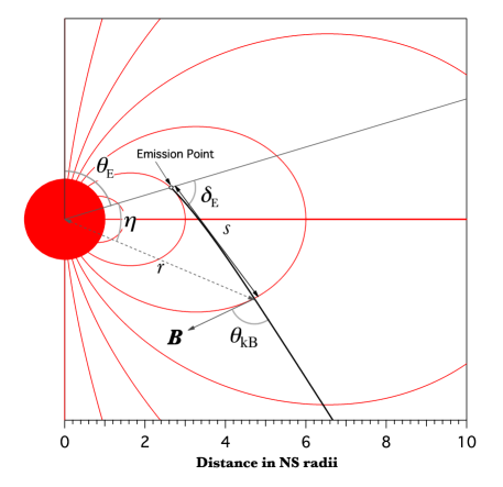
Figure 1.— Photon propagation geometry in a dipole magnetic field, with red curves representing field lines. The photon emission point is at an altitude $\,r_{\hbox{\sixrm E}}=hR_{\hbox{\sixrm NS}}\,$ and colatitude $\,\theta_{\hbox{\sixrm E}}\,$. The photon trajectory, represented by the black line, is a straight line for flat spacetime and a curved path (shown here) for general relativistic considerations. At any location along the photon path, $\,\mathbf{k}\,$ is the photon momentum vector, and $\,\mathbf{B}\,$ is the local magnetic field vector; the angle between these two vectors is $\,\theta_{\hbox{\sevenrm kB}}\,$, given in Eq. (14). All such locations are defined by the propagation angle $\,\eta\,$, with the radial position $\,r\,$ relative to the center of the neutron star, and the distance $\,s\,$ from the point of emission being described by Equations (11) and (13), respectively.

The geometry for general spacetime trajectories used in the computation of $\,\tau\,$ is illustrated in Fig. 1. While slight curvature in the photon path is depicted so as to encapsulate the general relativistic study in Sec. 4, this curvature can be presumed to be zero for the present considerations of flat spacetime. Each of the angles in this diagram can be defined once the emission colatitude $\,\theta_{\hbox{\sixrm E}}\,$ and emission altitude $\,r_{\hbox{\sixrm E}}=hR_{\hbox{\sixrm NS}}\,$ are specified. The instantaneous colatitude $\,\theta\,$ with respect to the magnetic axis is

$$\theta\;=\;\eta+\theta_{\hbox{\sixrm E}}\quad.$$ (8)

This defines the propagation angle $\,\eta\,$, which is the angle between the radial vector at the time of emission and the radial vector at the present photon position. The photon trajectory initially starts parallel to the magnetic field, since gamma-rays in pulsars are necessarily emitted by ultra-relativistic electrons that move basically along field lines. Standard models of electron acceleration invoke electrostatic potentials parallel to the local B (e.g. Sturrock 1971; Ruderman & Sutherland 1975; Daugherty & Harding 1982), and velocity drifts across B due to pulsar rotation are generally much smaller than $\,c\,$ for young gamma-ray pulsars. Accordingly, gamma-rays produced by primary electrons of Lorentz factor $\,\gamma_{e}\,$ are beamed to within a small Lorentz cone of half angle $\,\sim 1/\gamma_{e}\,$ centered along B. This restriction conveniently simplifies the trajectory parameter space, so that the angle between the radial direction and the photon trajectory at the point of emission, $\,\delta_{\hbox{\sixrm E}}\,$ (Gonthier & Harding 1994 name this $\,\delta_{0}\,$), is determined only by the colatitude $\,\theta_{\hbox{\sixrm E}}\,$ at the point of emission. The magnetic field vector at any point in a flat spacetime dipole magnetosphere is given by

$$\mathbf{B}\;=\;\hbox{${{\displaystyle B_{p}R_{\hbox{\sixrm NS}}^{3}\vphantom{(}}\over{\displaystyle 2r^{3}\vphantom{(}}}$}\left\{2\cos\theta\,\hat{r}+\sin\theta\,\hat{\theta}\right\}\quad.$$ (9)

where $\,B_{p}\,$ is the surface polar magnetic field, i.e., that at $\,r=R_{\hbox{\sixrm NS}}\,$ and $\,\theta=0\,$. The geometry of Fig. 1 then simply sets

$$\tan\delta_{\hbox{\sixrm E}}\;=\;\hbox{${{\displaystyle 1\vphantom{(}}\over{\displaystyle 2\vphantom{(}}}$}\tan\theta_{\hbox{\sixrm E}}\quad.$$ (10)

This result is, of course, independent of the altitude of emission. One remaining piece of the geometry is the relationship between the altitude along the photon path, and the angle $\,\eta\,$. This is simply derived using the trigonometric law of sines. Given $\,\delta_{\hbox{\sixrm E}}\,$, the dimensionless distance from the center of the neutron star $\,\chi=r/r_{\hbox{\sixrm E}}\,$, scaled by the altitude of emission, satisfies

$$\chi\;\equiv\;\hbox{${{\displaystyle r\vphantom{(}}\over{\displaystyle r_{\hbox{\sixrm E}}\vphantom{(}}}$}\;=\;\hbox{${{\displaystyle\sin\delta_{\hbox{\sixrm E}}\vphantom{(}}\over{\displaystyle\sin(\delta_{\hbox{\sixrm E}}-\eta)\vphantom{(}}}$}\quad.$$ (11)

This is the locus of a straight line in polar coordinates, and it is trivially determined that $\,\eta\to\delta_{\hbox{\sixrm E}}\,$ as $\,r\to\infty\,$. The photon momentum vector $\,\mathbf{k}\,$ along this path satisfies $\,\hat{\mathbf{k}}\equiv\mathbf{k}/\omega=\cos(\delta_{\hbox{\sixrm E}}-\eta)\hat{r}+\sin(\delta_{\hbox{\sixrm E}}-\eta)\hat{\theta}\,$.

For flat spacetime geometry with no aberration influences, it is convenient to restate the optical depth integral in Eq. (7) using the propagation angle $\,\eta\,$ as the integration variable:

$$\tau(l)\;=\;\hbox{${{\displaystyle\alpha_{f}\vphantom{(}}\over{\displaystyle\lambda\hbox to0.0pt{\hss--}_{c}\vphantom{(}}}$}\int_{0}^{\eta(l)}B\sin\theta_{\hbox{\sevenrm kB}}\,{\cal{F}}(\omega_{\perp},B)\hbox{${{\displaystyle ds\vphantom{(}}\over{\displaystyle d\eta\vphantom{(}}}$}\,d\eta\quad.$$ (12)

The propagation distance $\,s\,$ is easily found using the trigonometric law of sines, and thereby yields the change of variables Jacobian $\,ds/d\eta\,$ in Eq. (12):

$$s\;=\;\hbox{${{\displaystyle r_{\hbox{\sixrm E}}\,\sin\eta\vphantom{(}}\over{\displaystyle\sin(\delta_{\hbox{\sixrm E}}-\eta)\vphantom{(}}}$}\quad\Rightarrow\quad\hbox{${{\displaystyle ds\vphantom{(}}\over{\displaystyle d\eta\vphantom{(}}}$}\;=\;\hbox{${{\displaystyle r_{\hbox{\sixrm E}}\,\sin\delta_{\hbox{\sixrm E}}\vphantom{(}}\over{\displaystyle\sin^{2}(\delta_{\hbox{\sixrm E}}-\eta)\vphantom{(}}}$}\quad.$$ (13)

Therefore, the relationship for $\,\eta(l)\,$ is the inversion of Eq. (13) for $\,s=l\,$, i.e., $\,\tan\eta=\sin\delta_{\hbox{\sixrm E}}/(\cos\delta_{\hbox{\sixrm E}}+r_{\hbox{\sixrm E}}/l)\,$. The integrand in Eq. (12) includes a dependence on the angle $\,\theta_{\hbox{\sevenrm kB}}\,$ between the photon trajectory and the local magnetic field, particularly through the attenuation coefficient function $\,{\cal F}\,$. The photons start with $\,\theta_{\hbox{\sevenrm kB}}=0\,$, and this angle increases at first linearly as the photon propagates outward. The angle $\,\theta_{\hbox{\sevenrm kB}}\,$ is given geometrically by

$$\sin\theta_{\hbox{\sevenrm kB}}\;=\;\hbox{${{\displaystyle|\mathbf{k}\times\mathbf{B}|\vphantom{(}}\over{\displaystyle|k|.|B|\vphantom{(}}}$}\;=\;\hbox{${{\displaystyle{\hat{k}}_{r}B_{\theta}-{\hat{k}}_{\theta}B_{r}\vphantom{(}}\over{\displaystyle|B|\vphantom{(}}}$}\;=\;\hbox{${{\displaystyle\sin\theta\cos(\delta_{\hbox{\sixrm E}}-\eta)-2\cos\theta\sin(\delta_{\hbox{\sixrm E}}-\eta)\vphantom{(}}\over{\displaystyle\sqrt{1+3\cos^{2}\theta}\vphantom{(}}}$}$$ (14)

at every point along the photon’s path. Using Eq. (10) simply demonstrates that the right hand side of this expression approaches zero as $\,\eta=\theta-\theta_{\hbox{\sixrm E}}\to 0\,$. Note also that by forming $\,\cos\theta_{\hbox{\sevenrm kB}}\,$ and using Eq. (11), one can show routinely that this result is equivalent to Eq. (5) of Baring & Harding (2007). In the limit of small colatitudes near the magnetic axis, one simply derives $\,\sin\theta_{\hbox{\sevenrm kB}}\approx 3\eta/2\,$, which can be combined with $\,r/r_{\hbox{\sixrm E}}\approx 1+2\eta/\theta_{\hbox{\sixrm E}}\,$ to yield $\,\theta_{\hbox{\sevenrm kB}}\approx 3\theta_{\hbox{\sixrm E}}(r/r_{\hbox{\sixrm E}}-1)/4\,$. This dependence closely approximates the low altitude values for $\,\theta_{\hbox{\sevenrm kB}}\,$ in flat spacetime exhibited in Fig. 5a of Gonthier & Harding (1994). This completes the general formalism for pair creation optical depth determination in Minkowski metrics.

3.1. Optical Depth for Emission Near the Magnetic Axis

In order to better understand the character of the optical depth integral, it is instructive to consider the case of a photon emitted at very small colatitudes. This situation is representative of much of the relevant parameter space for young gamma-ray pulsars; for example, the Crab pulsar has a polar cap half-angle of about $\,4.5^{\circ}\,$ and the Vela pulsar has a polar cap half-angle of about $\,2.8^{\circ}\,$. For these photons emitted very close to the magnetic axis, $\,\eta\,$ and $\,\theta_{\hbox{\sixrm E}}\,$ are small. In this limit, we have the approximations

$$B\;\approx\;\hbox{${{\displaystyle B_{p}(\delta_{\hbox{\sixrm E}}-\eta)^{3}\vphantom{(}}\over{\displaystyle h^{3}\delta_{\hbox{\sixrm E}}^{3}\vphantom{(}}}$}\quad,\quad\sin\theta_{\hbox{\sevenrm kB}}\;\approx\;\hbox{${{\displaystyle 3\vphantom{(}}\over{\displaystyle 2\vphantom{(}}}$}\,\eta$$ (15)

for $\,r_{\hbox{\sixrm E}}=hR_{\hbox{\sixrm NS}}\,$. We also have $\,ds/d\eta\approx r_{\hbox{\sixrm E}}\delta_{\hbox{\sixrm E}}/(\delta_{\hbox{\sixrm E}}-\eta)^{2}\,$ using Eq. (13), with $\,\delta_{\hbox{\sixrm E}}\approx\theta_{\hbox{\sixrm E}}/2\,$. These results can be inserted into Eq. (12), and the integration variable changed to $\,x=\eta/\delta_{\hbox{\sixrm E}}\,$, yielding an approximation for the optical depth in axial locales:

$$\tau(l)\;\approx\;\hbox{${{\displaystyle 3\theta_{\hbox{\sixrm E}}\vphantom{(}}\over{\displaystyle 4\vphantom{(}}}$}\,\hbox{${{\displaystyle B_{p}\vphantom{(}}\over{\displaystyle h^{2}\vphantom{(}}}$}\hbox{${{\displaystyle\alpha_{f}R_{\hbox{\sixrm NS}}\vphantom{(}}\over{\displaystyle\lambda\hbox to0.0pt{\hss--}\vphantom{(}}}$}\int_{8/(3\theta_{\hbox{\sixrm E}}\varepsilon)}^{x_{+}}x(1-x)\,{\cal F}\left(\hbox{${{\displaystyle 3\vphantom{(}}\over{\displaystyle 4\vphantom{(}}}$}\,\varepsilon\theta_{\hbox{\sixrm E}}x,\,\hbox{${{\displaystyle B_{p}\vphantom{(}}\over{\displaystyle h^{3}\vphantom{(}}}$}\left[1-x\right]^{3}\right)dx\;\;,\quad x_{+}\;=\;\hbox{${{\displaystyle l\vphantom{(}}\over{\displaystyle l+hR_{\hbox{\sixrm NS}}\vphantom{(}}}$}\;\;.$$ (16)

This form is applicable to any choice of the pair conversion function $\,{\cal F}\,$. Observe that here the the local energy $\,\omega\,$ has been replaced with the energy $\,\varepsilon\,$ seen by an observer at infinity; the two are equivalent in flat spacetime with no rotation, but when we consider general relativity and aberration, the distinction will become important. The upper limit $\,x_{+}\,$ is the value of $\,x=\eta/\delta_{\hbox{\sixrm E}}\,$ that realizes a path length $\,l\,$, and is well approximated by $\,l/\left(l+hR_{\hbox{\sixrm NS}}\right)\,$ near the magnetic axis. The lower limit defines the threshold condition, so that if $\,\varepsilon\theta_{\hbox{\sixrm E}}\leq 8/3\,$, propagation in flat spacetime out of the magnetosphere never moves the photon above the pair threshold at $\,\omega_{\perp}=2\,$, and $\,\tau=0\,$ over the entire photon trajectory. For the particular choice of Erber’s (1966) attenuation coefficient in Eq. (2), the integral for the optical depth assumes a fairly simple form:

$$\tau_{\hbox{\sevenrm Erb}}(l)\;\approx\;\hbox{${{\displaystyle 9\sqrt{3}\,\theta_{\hbox{\sixrm E}}\vphantom{(}}\over{\displaystyle 64\sqrt{2}\vphantom{(}}}$}\,\hbox{${{\displaystyle B_{p}\vphantom{(}}\over{\displaystyle h^{2}\vphantom{(}}}$}\hbox{${{\displaystyle\alpha_{f}R_{\hbox{\sixrm NS}}\vphantom{(}}\over{\displaystyle\lambda\hbox to0.0pt{\hss--}\vphantom{(}}}$}\int_{8/(3\theta_{\hbox{\sixrm E}}\varepsilon)}^{x_{+}}x(1-x)\,\exp\left\{-\hbox{${{\displaystyle 32h^{3}\vphantom{(}}\over{\displaystyle 9\varepsilon B_{p}\theta_{\hbox{\sixrm E}}\vphantom{(}}}$}\hbox{${{\displaystyle 1\vphantom{(}}\over{\displaystyle x(1-x)^{3}\vphantom{(}}}$}\right\}dx\quad.$$ (17)

If one considers emission points near the magnetic axis at different altitudes along a particular field line with a footpoint colatitude $\,\theta_{f}\,$, then $\,\theta_{\hbox{\sixrm E}}\approx\theta_{f}\sqrt{h}\,$ gives the altitude dependence of the emission colatitude. Exploring attenuation opacity along a fixed field line is germane to treating gamma-ray emission that takes place along or near the last open field line, where $\,\theta_{f}\,$ is fixed by the pulsar’s rotational period. The escape energy $\,\varepsilon_{\rm esc}\,$ can be computed by setting $\,\tau(\infty)=1\,$, for which $\,x_{+}\to 1\,$. Imposing this $\,\tau(\infty)=1\,$ criterion, and presuming $\,\varepsilon\theta_{\hbox{\sixrm E}}\gg 1\,$ in Eq. (17), yields the approximate altitude dependence

$$\varepsilon_{\rm esc}\;\propto\;h^{5/2}$$ (18)

for the escape energy. This is a flat spacetime result for near polar axis locales that was identified by Zhang & Harding (2000; see also Lee, et al. 2010). Deviations from this simple altitude dependence arise (i) when the footpoint colatitude $\,\theta_{f}\,$ is not sufficiently small, (ii) if the pair conversion occurs not very far from the $\,\omega_{\perp}=2\,$ threshold, and (iii) down near the stellar surface where general relativistic effects modify the values of $\,\omega\,$, $\,B\,$ and $\,\theta_{\hbox{\sevenrm kB}}\,$.

For significantly sub-critical $\,B_{p}\,$, a complete asymptotic expression for the optical depth after propagation to high altitudes can be determined using the method of steepest descents to compute the integral for $\,\tau(l)\,$, since the integrand in Eq. (17) is exponentially sensitive to values of $\,x\,$. This is precisely the method employed by Arons & Scharlemann (1979) and later adopted by Hibschman & Arons (2001) in developing similar opacity integrations. The exponential realizes a very narrow peak at $\,x=1/4\,$, so that for $\,l\to\infty\,$ and $\,x_{+}=1\,$

$$\tau_{\hbox{\sevenrm Erb}}(l)\;\approx\;\hbox{${{\displaystyle 3^{6}\vphantom{(}}\over{\displaystyle 2^{19}\vphantom{(}}}$}\left(\hbox{${{\displaystyle 3\pi\varepsilon B_{p}^{3}\theta_{f}^{3}\vphantom{(}}\over{\displaystyle 2h^{11/2}\vphantom{(}}}$}\right)^{1/2}\hbox{${{\displaystyle\alpha_{f}R_{\hbox{\sixrm NS}}\vphantom{(}}\over{\displaystyle\lambda\hbox to0.0pt{\hss--}\vphantom{(}}}$}\exp\left\{-\hbox{${{\displaystyle 2^{13}h^{5/2}\vphantom{(}}\over{\displaystyle 3^{5}\varepsilon B_{p}\theta_{f}\vphantom{(}}}$}\right\}\quad.$$ (19)

This result actually applies for any $\,x_{+}>1/4\,$, i.e. when $\,l\gtrsim hR_{\hbox{\sixrm NS}}/3\,$. It is independent of $\,l\,$ since the integrand has sampled beyond the peak and has shrunk to very small values when $\,x\,$ exceeds $\,1/4\,$ by a significant amount. Eq. (19) is in agreement with the approximate optical depth computed by Hibschman & Arons (2001) in their Eq. (8), which was similarly formulated to treat gamma-ray propagation above the magnetic pole. Note that Arons & Scharlemann (1979) provided a more general opacity integral by treating magnetic multipole configurations. Again setting $\,\tau_{\hbox{\sevenrm Erb}}(\infty)=1\,$, and taking logarithms of Eq. (19), the escape energy $\,\varepsilon_{\rm esc}\,$ for the Erber attenuation coefficient satisfies

$$\varepsilon_{\rm esc}\;=\;\hbox{${{\displaystyle 2^{13}h^{5/2}\vphantom{(}}\over{\displaystyle 3^{5}B_{p}\theta_{f}\vphantom{(}}}$}\left\{\log_{e}\left(\hbox{${{\displaystyle 3^{6}\vphantom{(}}\over{\displaystyle 2^{19}\vphantom{(}}}$}\,\hbox{${{\displaystyle\alpha_{f}R_{\hbox{\sixrm NS}}\vphantom{(}}\over{\displaystyle\lambda\hbox to0.0pt{\hss--}\vphantom{(}}}$}\right)+\hbox{${{\displaystyle 1\vphantom{(}}\over{\displaystyle 2\vphantom{(}}}$}\log_{e}\hbox{${{\displaystyle 3\pi\varepsilon_{\rm esc}B_{p}^{3}\theta_{f}^{3}\vphantom{(}}\over{\displaystyle 2h^{11/2}\vphantom{(}}}$}\right\}^{-1}\quad.$$ (20)

While an exact solution for $\,\varepsilon_{\rm esc}\,$ must be determined numerically from this transcendental equation, the second logarithmic term on the right is only weakly dependent on its arguments. Therefore, to a good approximation, one can infer that $\,\varepsilon_{\rm esc}\propto 1/B_{p}\,$ and $\,\varepsilon_{\rm esc}\propto 1/\theta_{f}\,$, both of which emerge due to the presence of the factor $\,\omega_{\perp}B\,$ in the argument of the exponential in Erber’s asymptotic form.

The same protocol can be adopted for pair conversion rates that include threshold modifications, specifically Eq. (3). In this case, as the counterpart of Eq. (16) we have

$$\tau(l)\;\approx\;\hbox{${{\displaystyle 3\theta_{\hbox{\sixrm E}}\vphantom{(}}\over{\displaystyle 4\vphantom{(}}}$}\,\hbox{${{\displaystyle B_{p}\vphantom{(}}\over{\displaystyle h^{2}\vphantom{(}}}$}\hbox{${{\displaystyle\alpha_{f}R_{\hbox{\sixrm NS}}\vphantom{(}}\over{\displaystyle\lambda\hbox to0.0pt{\hss--}\vphantom{(}}}$}\int_{8/(3\theta_{\hbox{\sixrm E}}\varepsilon)}^{x_{+}}x(1-x)\,{\cal F}_{\rm BK07}\left(\hbox{${{\displaystyle 3\vphantom{(}}\over{\displaystyle 4\vphantom{(}}}$}\,\varepsilon\theta_{\hbox{\sixrm E}}x,\,\hbox{${{\displaystyle B_{p}\vphantom{(}}\over{\displaystyle h^{3}\vphantom{(}}}$}\left[1-x\right]^{3}\right)dx\quad,$$ (21)

again for $\,x_{+}=l/(l+hR_{\hbox{\sixrm NS}})\,$. We can simplify the ensuing analysis by making the substitution $\,\lambda=3\theta_{\hbox{\sixrm E}}\varepsilon/8\geq 1\,$ so that locally $\,\omega_{\perp}=2\lambda x\,$ along the trajectory. The argument of the exponential is of the form $\,h^{3}q(x,\,\lambda)/B_{p}\,$ where

$$q(x,\,\lambda)\;\equiv\;\hbox{${{\displaystyle\phi(2\lambda x)\vphantom{(}}\over{\displaystyle 4(1-x)^{3}\vphantom{(}}}$}\;=\;-\hbox{${{\displaystyle 2\lambda x\vphantom{(}}\over{\displaystyle(1-x)^{3}\vphantom{(}}}$}-\hbox{${{\displaystyle\left(\lambda x\right)^{2}-1\vphantom{(}}\over{\displaystyle(1-x)^{3}\vphantom{(}}}$}\log_{e}\left(\hbox{${{\displaystyle\lambda x-1\vphantom{(}}\over{\displaystyle\lambda x+1\vphantom{(}}}$}\right)$$ (22)

Using the method of steepest descents once again, we take the first derivative of the function in the exponential, and set it equal to zero to find the peak of the function. The solution of $\,\partial q/\partial x=0\,$ is a transcendental function in $\,\lambda\,$, but it can be numerically approximated to better than 3% by

$$\overline{x}\approx\frac{1}{4}+0.82\lambda^{-5/3}.$$ (23)

Given $\partial q/\partial x=0$, the logarithmic term $\,\log_{e}[(\lambda\overline{x}-1)/(\lambda\overline{x}+1)]\,$ can be expressed algebraically, and $q^{\prime\prime}(x,\lambda)$ can be written in the following form:

$$q^{\prime\prime}(\overline{x},\lambda)\;=\;\frac{8\lambda\left[\lambda^{2}\left(2\overline{x}^{3}-3\overline{x}+1\right)-3\overline{x}+3\right]}{(\lambda^{2}\overline{x}(\overline{x}+2)-3)(1-\overline{x})^{5}(\lambda^{2}\overline{x}^{2}-1)}\quad.$$ (24)

The integral is then given approximately, as before, by the method of steepest descents. With some cancellation, we then obtain

$$\tau_{\hbox{\sevenrm BK07}}\;\approx\;\frac{\alpha_{f}R_{\hbox{\sixrm NS}}}{\lambda\hbox to0.0pt{\hss--}}\frac{[3(\lambda\overline{x})^{2}-1]\,(\lambda\overline{x}-1)}{2\varepsilon\,\lambda^{2}\overline{x}\,(\lambda\overline{x}+1)}\left[\frac{\pi\chi^{3}B_{p}^{3}}{2(\overline{x}+2)\,(1-\overline{x})\,|\Upsilon|\,h^{7}}\right]^{1/2}\exp\left\{-\frac{h^{3}}{B_{p}\chi}\right\}$$ (25)

where

$$\Upsilon\;=\;\left(1-2\overline{x}-2\overline{x}^{2}\right)+\hbox{${{\displaystyle 3\vphantom{(}}\over{\displaystyle\lambda^{2}\vphantom{(}}}$}\quad,\quad\chi\;=\;\hbox{${{\displaystyle(1-\overline{x})^{2}\vphantom{(}}\over{\displaystyle 4\lambda\vphantom{(}}}$}\,\Bigl{\{}\lambda^{2}\overline{x}(\overline{x}+2)-3\Bigr{\}}\quad.$$ (26)

Here $\,\Upsilon\,$ is employed to render the $\,q^{\prime\prime}(\overline{x},\,\lambda)\,$ term more compact, and $\,\chi=1/q(\overline{x},\,\lambda)\,$. Noting that $\,\theta_{f}\approx 8\lambda/(3\varepsilon\sqrt{h})\,$ in this small colatitude limit, Eq. (25) agrees with the Erber approximation in Eq. (19) to high precision in the regime where $\,\lambda\rightarrow\infty\,$, and exhibits the appropriate threshold behavior. Setting $\,\tau(\infty)=1\,$ gives a transcendental equation that can be solved numerically for $\,\varepsilon_{\rm esc}\,$. The impressive precision of this analytic steepest descents result for the escape energy is apparent in Fig. 3 below.

Well above the escape energy, the pair attenuation length $\,l\,$ is far inferior to the neutron star radius. For surface emission ($\,h=1\,$), in this $\,l\ll R_{\hbox{\sixrm NS}}\,$ limit, we can assert $\,x_{+}\ll 1\,$ in Eq. (16), so that series expansion in the $\,x\,$ integration variable yields

$$\tau(l)\;\approx\;\hbox{${{\displaystyle 3\theta_{\hbox{\sixrm E}}\vphantom{(}}\over{\displaystyle 4\vphantom{(}}}$}\,\hbox{${{\displaystyle\alpha_{f}R_{\hbox{\sixrm NS}}\vphantom{(}}\over{\displaystyle\lambda\hbox to0.0pt{\hss--}\vphantom{(}}}$}\,B_{p}\int_{8/(3\theta_{\hbox{\sixrm E}}\varepsilon)}^{x_{+}}x\,{\cal F}\left(\hbox{${{\displaystyle 3\vphantom{(}}\over{\displaystyle 4\vphantom{(}}}$}\,\varepsilon\theta_{\hbox{\sixrm E}}x,\,B_{p}\left[1-3x\right]\right)dx\quad,\quad x_{+}\;\ll\;1\quad.$$ (27)

Analytic reduction of this integral is fairly complicated for the case of the $\,{\cal F}_{\rm B88}\,$ rate, but is relatively amenable for the Erber form, which we employ at this juncture. Inserting Eq. (2) for $\,{\cal F}\,$, because of the strong exponential dependence of the integrand, the dominant contribution to the integral comes from $\,x\approx x_{+}\,$. Replacing the factor of $\,x\,$ in the integrand that lies outside the exponential by $\,x_{+}^{3}/x^{2}\,$, for $\,x_{+}\approx l/R_{\hbox{\sixrm NS}}\,$, yields

$$\tau(l)\;\approx\;\hbox{${{\displaystyle 9\sqrt{3}\,B_{p}\theta_{\hbox{\sixrm E}}\vphantom{(}}\over{\displaystyle 64\sqrt{2}\vphantom{(}}}$}\,\hbox{${{\displaystyle\alpha_{f}R_{\hbox{\sixrm NS}}\vphantom{(}}\over{\displaystyle\lambda\hbox to0.0pt{\hss--}\vphantom{(}}}$}\,\left(\hbox{${{\displaystyle l\vphantom{(}}\over{\displaystyle R_{\hbox{\sixrm NS}}\vphantom{(}}}$}\right)^{3}\,\,\exp\left\{\hbox{${{\displaystyle 32\vphantom{(}}\over{\displaystyle 3\varepsilon B_{p}\theta_{\hbox{\sixrm E}}\vphantom{(}}}$}\right\}\int_{8/(3\theta_{\hbox{\sixrm E}}\varepsilon)}^{x_{+}}\,\exp\left\{-\hbox{${{\displaystyle 32\vphantom{(}}\over{\displaystyle 9\varepsilon B_{p}\theta_{\hbox{\sixrm E}}\vphantom{(}}}$}\hbox{${{\displaystyle 1\vphantom{(}}\over{\displaystyle x\vphantom{(}}}$}\right\}\hbox{${{\displaystyle dx\vphantom{(}}\over{\displaystyle x^{2}\vphantom{(}}}$}\quad.$$ (28)

This manipulation affords analytic evaluation of the integral. The attenuation length $\,L\,$ is obtained by setting $\,\tau(L)=1\,$ in the resulting equation for $\,\tau(l)\,$, which after rearrangement leads to

$$\exp\left\{-\hbox{${{\displaystyle 32R_{\hbox{\sixrm NS}}\vphantom{(}}\over{\displaystyle 9\varepsilon B_{p}\theta_{\hbox{\sixrm E}}L\vphantom{(}}}$}\right\}\;\approx\;\hbox{${{\displaystyle 2048\sqrt{2}\vphantom{(}}\over{\displaystyle 81\sqrt{3}\,\varepsilon B_{p}^{2}\theta_{\hbox{\sixrm E}}^{2}\vphantom{(}}}$}\,\hbox{${{\displaystyle\lambda\hbox to0.0pt{\hss--}\vphantom{(}}\over{\displaystyle\alpha_{f}R_{\hbox{\sixrm NS}}\vphantom{(}}}$}\,\left(\hbox{${{\displaystyle R_{\hbox{\sixrm NS}}\vphantom{(}}\over{\displaystyle L\vphantom{(}}}$}\right)^{3}\,\exp\left\{-\hbox{${{\displaystyle 32\vphantom{(}}\over{\displaystyle 3\varepsilon B_{p}\theta_{\hbox{\sixrm E}}\vphantom{(}}}$}\right\}+\exp\left\{-\hbox{${{\displaystyle 4\vphantom{(}}\over{\displaystyle 3B_{p}\vphantom{(}}}$}\right\}\quad.$$ (29)

In general, solutions for $\,L\,$ are realized when the second exponential term on the right hand side of Eq. (29) can be neglected, at the $\,<10^{-3}\,$ level. This simplifies the algebra, and taking logarithms, one arrives at

$$\hbox{${{\displaystyle R_{\hbox{\sixrm NS}}\vphantom{(}}\over{\displaystyle L\vphantom{(}}}$}\;\approx\;3+\hbox{${{\displaystyle 9\varepsilon B_{p}\theta_{\hbox{\sixrm E}}\vphantom{(}}\over{\displaystyle 32\vphantom{(}}}$}\log_{e}\left[\hbox{${{\displaystyle 81\sqrt{3}\,\varepsilon B_{p}^{2}\theta_{\hbox{\sixrm E}}^{2}\vphantom{(}}\over{\displaystyle 2048\sqrt{2}\vphantom{(}}}$}\,\hbox{${{\displaystyle\alpha_{f}L^{3}\vphantom{(}}\over{\displaystyle\lambda\hbox to0.0pt{\hss--}R_{\hbox{\sixrm NS}}^{2}\vphantom{(}}}$}\right]\quad.$$ (30)

This transcendental equation must be solved numerically, though the general trend is given approximately by $\,L\propto(\varepsilon\theta_{\hbox{\sixrm E}})^{-1}\,$ when $\,L\ll R_{\hbox{\sixrm NS}}\,$, since the dependence on parameters inside the logarithmic term is weak. This compact analytic derivation nicely describes the attenuation length values for the Erber rate, as is evident in Fig. 2.

The general character of the attenuation length solutions for the full $\,{\cal F}_{\rm BK07}\,$ pair attenuation rate near threshold is depicted in Fig. 2, for a neutron star radius of $\,R_{\hbox{\sixrm NS}}=10^{6}\,$cm. Note that computations (not shown) that also include the polarization-averaged forms for the first two “sawtooth” peaks [see Sec. 2] in the exact attenuation coefficient formula of Daugherty and Harding (1983) generate attenuation lengths that are almost indistinguishable from those shown, even for $\,B_{p}=1\,$. The attenuation length curves are declining functions of the photon energy, generally with the expected $\,L\propto 1/\varepsilon\,$ dependence when $\,L\ll R_{\hbox{\sixrm NS}}\,$. While they illustrate the particular case of surface emission from a colatitude of $\,\theta_{\hbox{\sixrm E}}\approx 5.72^{\circ}\,$, i.e. close to the polar cap colatitude for the Crab pulsar, at high energies, our calculations also reveal roughly $\,L\propto 1/\theta_{\hbox{\sixrm E}}\,$ behavior for a range of non-equatorial emission colatitudes.

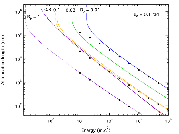
Figure 2.— The pair attenuation length $\,L\,$ (satisfying the criterion $\,\tau(L)=1\,$) of photons emitted from the neutron star surface ($\,h=1\,$) in flat spacetime, plotted as a function of photon energy. The emission colatitude is $\,0.1\,$radian. The curves are labeled with the surface polar magnetic field, $\,B_{p}\,$, scaled by the quantum critical field. Solid curves represent lengths computed using the integral calculation of the optical depth in Eq. (21), i.e. they employ the approximation derived by Baier & Katkov (2007); see Sec. 2 for details. Dashed lines depict the attenuation lengths computed from Eq. (17) using Erber’s (1966) reaction rate. The large black dots display the approximate form of the attenuation length encapsulated in Eq. (30) for the cases of $\,B_{p}=0.01\,$, $\,B_{p}=0.1\,$ and $\,B_{p}=1\,$, thereby highlighting its high level of precision when $\,L\ll R_{\hbox{\sixrm NS}}=10^{6}\,$cm.

Since the pair attenuation rate increases rapidly with magnetic field strength, the attenuation length declines with increasing $\,B_{p}\,$, roughly as $\,1/B_{p}\,$ in accordance with Eq. (30) for $\,B_{p}\lesssim 0.1\,$. However, as the magnetic field of the pulsar approaches $\,B_{\rm cr}\,$, photon attenuation occurs for angles $\,\theta_{\hbox{\sevenrm kB}}\,$ closer to the absolute pair creation threshold of $\,\varepsilon\sin\theta_{\hbox{\sevenrm kB}}=2\,$, independent of the value of $\,B_{p}\,$. The attenuation length curves for $\,B_{p}=0.3\,$ and $\,B_{p}=1\,$ then become indistinguishable at intermediate energies $\,10^{2}\lesssim\varepsilon\lesssim 10^{4}\,$ because the attenuation coefficients just above the pair creation threshold are so large that the distances traveled by the photons after they cross the threshold are minuscule in comparison with the propagation distance required to reach the threshold. At the very highest energies, the $\,B_{p}=0.3\,$ and $\,B_{p}=1\,$ curves begin to diverge again because the attenuation coefficients drop by several orders of magnitude and the distance a $\,B_{p}=0.3\,$ photon travels after crossing the threshold before converting becomes comparable to the distance it transits before reaching the point where $\,\varepsilon\sin\theta_{\hbox{\sevenrm kB}}=2\,$.

The dashed curves display the attenuation lengths for Erber rate formalism [see Eq. (17)]. Since the Erber form significantly overestimates the attenuation coefficient near pair threshold, it generates shorter attenuation lengths than does the more precise determination using Eq. (21). The analytic approximation in Eq. (30) to the Erber $\,\tau(L)=1\,$ formalism is also shown as discrete dots, demonstrating a good precision in matching the fully numerical curves at high energies. This approximation provides a useful guide to the generic character of attenuation in $\,L\ll R_{\hbox{\sixrm NS}}\,$ domains. The vertical upturns in the curves at low energies define the photon escape energies $\,\varepsilon_{\rm esc}\,$ for each $\,B_{p}\,$ case; such features are the focus of Section 3.2, and demarcate the energy domains for pair creation transparency of the magnetosphere.

3.2. Pair Creation Escape Energies in Flat Spacetime

The focus now turns to the escape energies, since they provide upper bounds to the spectral window of pair transparency for neutron star magnetospheres. Numerical solutions of Eq. (12) in the limit $\,l\to\infty\,$ can help gain a better understanding of where the effects of magnetic pair creation will be the strongest. By specifying emission at the surface ($\,h=1\,$), fixing a surface polar magnetic field $\,B_{p}\,$ and then solving for $\,\varepsilon_{\rm esc}\,$ as a function of the colatitude of emission $\,\theta_{\hbox{\sixrm E}}\,$, we obtain the plot shown in Fig. 3. The core results are contained in the solid curves, which express the $\,\tau(\infty)=1\,$ criterion using the $\,{\cal F}_{\rm BK07}\,$ attenuation coefficient derived by Baier & Katkov (2007), in concert with the polarization-averaged forms for $\,{\cal F}\,$ that include the first two “sawtooth” peaks in the exact attenuation coefficient formula expressed in Eqs. (5) and (6). We can see that for small colatitudes, $\,\varepsilon_{\rm esc}\propto 1/\theta_{\hbox{\sixrm E}}\,$ and $\,\varepsilon_{\rm esc}\propto 1/B_{p}\,$, as expected from Eq. (20). The dashed lines representing the steepest descents approximation in Eq. (25) clearly illustrate the remarkable accuracy of this expression over a wide range of colatitudes and subcritical fields. The effects of threshold corrections are also apparent from this Figure. For the purple $\,B_{p}=1\,$ curves, the Erber approximation (short dotted purple line) to the attenuation coefficient produces escape energies nearly a factor of 3 below the threshold-corrected result. For lower magnetic fields, pair creation is taking place well above threshold, and the Erber curves are much closer to the threshold-corrected curves. Note that the analysis of Lee et al. (2010) omits consideration of threshold influences in the pair production rates, and thereby would underestimate $\,\varepsilon_{\rm esc}\,$ when the critical field is approached.

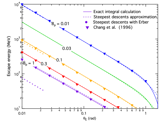
Figure 3.— The maximum energy $\,\varepsilon_{\rm esc}\,$ of photons emitted from the neutron star surface ($\,h=1\,$) that can escape to infinity in flat spacetime, plotted as a function of emission colatitude. The curves are labeled with the surface polar magnetic field, $\,B_{p}\,$, scaled by the quantum critical field. Solid curves represent results for $\,\tau(\infty)=1\,$ using the integral calculation of the optical depth in Eq. (16). This determination employs polarization-averaged forms for $\,{\cal F}\,$ that include the first two “sawtooth” peaks in the exact attenuation coefficient formula of Daugherty and Harding (1983), and at higher $\,\omega_{\perp}\,$ uses the approximation derived by Baier & Katkov (2007); see Sec. 2 for details. Dashed lines represent the $\,\tau(\infty)=1\,$ determination using the steepest descents approximation in Eq. (25), and the short dotted lines depict the asymptotic form in Eq. (20) obtained using Erber’s (1966) reaction rate, but only for $\,B_{p}=0.1\,$ and $\,B_{p}=1\,$. Triangles are taken from the computations illustrated in Fig. 2 of Chang et al. (1996), for comparison. Although the steepest descents approximation was calculated in the small colatitude limit, it remains extremely good out to moderate colatitudes before diverging from the exact determination when $\,\theta_{\hbox{\sixrm E}}\sim 1\,$.

In comparing with extant flat spacetime computations of escape energies, our results realize good agreement with Fig. 2 of Ho, Epstein & Fenimore (1990), using the Erber asymptotic form of Eq. (2); this matches their chosen attenuation coefficient closely. In this analysis, we assume that photons are always emitted parallel to the magnetic field, so comparison of our results is made to the topmost ($\,\psi_{i}=0\,$) curve of their Fig. 2, the x-axis of which is equivalent to $\,\log(\delta_{\hbox{\sixrm E}}+\theta_{\hbox{\sixrm E}})\,$ in our variables. For $\,B=2\times 10^{12}\,$Gauss, the apparent difference between our numerics and theirs is less than about 15% , though visual precision in reading this plot limits such an estimate. For the Erber attenuation coefficient in flat spacetime, multiplying the photon escape energy from a fixed emission altitude and colatitude by the surface polar magnetic field yields an approximately constant result.

If, on the other hand, one fixes the surface polar field and the photon energy, and calculates the lowest altitude $\,r_{\rm min}\,$ from which photons of that energy can escape to infinity, one can formulate a “pair convertosphere” plot like that in Fig. 4, which is computed for flat spacetime. The leaf-shaped curves represent a cross-section through a $\,\tau=1\,$ surface that is symmetric about the magnetic axis. Inside the surface, to a first approximation, all photons of the labeled energy will convert to pairs. Outside the surface, photons can escape and be detected. At a fixed colatitude, a higher altitude of emission results in a higher escape energy (corresponding to shifting the curves in Fig. 3 up in energy). In a Minkowski metric, all of these minimum altitude curves drop to below the stellar surface at the magnetic pole, since there the field line radius of curvature is very large, and photons do not quickly encounter significant $\,\theta_{\hbox{\sevenrm kB}}\,$ during propagation when initially emitted parallel to the local field. Rotational aberration influences, which will be considered in Section. 5 below, introduce an azimuthal asymmetry about the magnetic axis for an inclined pulsar, and significantly distort the shape of the surfaces near the magnetic poles, but not by much in equatorial regions. General relativistic influences (discussed in Section 4) are significant below $\,2R_{\hbox{\sixrm NS}}\,$, and while they do not appreciably alter the overall morphology of the leaf-shaped contours, they do force them to high slightly altitudes above the poles. Rotational aberration distorts the morphology of these $\,\tau=1\,$ curves somewhat, introducing asymmetry between the leading and trailing edges, along the lines of the magnetospheric cross section plot in Fig. 3 of Harding, Tademaru & Esposito (1978).

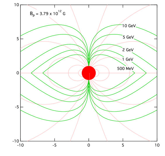
Figure 4.— “Pair convertosphere” diagram for a pulsar with the same magnetic field as the Crab, for flat spacetime and the specific case of no rotational/aberration influences. Dipolar field structure (depicted in light red) underlays each leaf-shaped green curve, which represents the lowest possible emission point at a given colatitude for a photon of a fixed energy (as labelled), below which magnetic pair creation would attenuate the photon before it could escape from the neutron star magnetosphere. The photons are always presumed to be emitted parallel to the local field. The scale is neutron star radii, with the unit radius circle in the center representing the neutron star. General relativistic effects alter these curves only very near the neutron star surface, and then only modestly, moving them to slightly higher altitudes.

As the pair convertosphere minimum altitude contours move to equatorial regions, it is clear that $\,r_{\rm min}\,$ is a monotonically increasing function of colatitude $\,\theta_{\hbox{\sixrm E}}\,$. Photons emitted above the equator more readily transit across the field lines than in polar locales, and so have shorter attenuation lengths. This is because the magnetic field lines possess shorter radii of curvature in equatorial zones than in polar regions, at a given emission altitude. Hence, for a fixed photon energy, in order to compensate and increase $\,L\,$ to infinity, the local field strengths sampled must be lowered, forcing the required $\,\theta_{\hbox{\sevenrm kB}}\,$ at the instant of conversion to larger values. Thus, the minimum altitudes must rise as $\,\theta_{\hbox{\sixrm E}}\,$ does, and the result is the leaf-shaped morphology in Fig. 3. For moderately small colatitudes, this trend can be discerned from Eq. (20), namely the Erber asymptotic form for the escape energy. It is noteworthy that this behavior contradicts that displayed in Figure 3 of Lee et al. (2010), where their $\,r_{\rm min}\,$ values drop for colatitudes $\,\theta\gtrsim 60^{\circ}\,$, a decline that does not appear to depend on aberrational influences in their work. It is not clear why this behavior is elicited in their computations. In Section 5, we demonstrate that rotational/aberrational influences on escape energy and minimum altitude determinations at these equatorial colatitudes are comparatively small.

4. GENERAL RELATIVISTIC EFFECTS

Our overall approach to calculating curved spacetime effects on photon attenuation will be to integrate the optical depth over path length intervals in the local inertial frame (hereafter LIF), with all magnetic fields, angles, energies, and distances computed in that frame. In general, we will use the definitions for curved spacetime quantities from Gonthier & Harding (1994, hereafter GH94), with the notation altered slightly for clarity. Our starting point is again Eq. (7), therefore requiring specification of the quantities $\,B\,$, $\,\omega\,$ and $\,\theta_{\hbox{\sevenrm kB}}\,$ in the LIF. The blueshift of the photon energy in the LIF from its value $\,\varepsilon\equiv\omega_{\infty}\,$ at infinity (i.e. as observed) can be accounted for with the simple correction

$$\omega\;=\;\hbox{${{\displaystyle\varepsilon\vphantom{(}}\over{\displaystyle\sqrt{1-\Psi}\vphantom{(}}}$}\quad,\quad\Psi\;=\;\hbox{${{\displaystyle r_{s}\vphantom{(}}\over{\displaystyle r\vphantom{(}}}$}\;\equiv\;\hbox{${{\displaystyle 2GM\vphantom{(}}\over{\displaystyle c^{2}r\vphantom{(}}}$}$$ (31)

at radius $\,r\,$, where $\,r_{s}=2GM/c^{2}\,$ is the Schwarzschild radius of a neutron star of mass $\,M\,$. The introduction of the dimensionless parameter $\,\Psi\,$ to describe the radial position will expedite the path length integration in curved spacetime constructs; we will use it as our integration variable instead of $\,\eta\,$ in Eq. (12), approximately equivalently to the approach of GH94. The emission altitude $\,r_{\hbox{\sixrm E}}\,$ will be prescribed by $\,\Psi_{\hbox{\sixrm E}}=r_{s}/r_{\hbox{\sixrm E}}<1\,$. Note that throughout, we will adopt the convention that $\,\varepsilon\,$ shall denote the dimensionless photon energy as seen by an observer, and $\,\omega\,$ shall signify that in the LIF.

The general relativistic form of a dipole magnetic field in a Schwarzschild metric was developed in Wasserman & Shapiro (1983). It is also expressed in Eq. (21) of GH94 in the LIF in terms of the coordinates $\,r\,$ and $\,\theta\,$ for an observer at infinity:

$$\hbox{\bf B}_{GR} = -\,3\,\hbox{${{\displaystyle B_{p}\cos\theta\vphantom{(}}\over{\displaystyle r_{s}^{2}r\vphantom{(}}}$}\left[\hbox{${{\displaystyle r\vphantom{(}}\over{\displaystyle r_{s}\vphantom{(}}}$}\log_{e}\left(1-\hbox{${{\displaystyle r_{s}\vphantom{(}}\over{\displaystyle r\vphantom{(}}}$}\right)+1+\hbox{${{\displaystyle r_{s}\vphantom{(}}\over{\displaystyle 2r\vphantom{(}}}$}\right]\hat{r}$$

$$+\,3\,\hbox{${{\displaystyle B_{p}\sin\theta\vphantom{(}}\over{\displaystyle r_{s}^{2}r\vphantom{(}}}$}\left[\left(\hbox{${{\displaystyle r\vphantom{(}}\over{\displaystyle r_{s}\vphantom{(}}}$}-1\right)\log_{e}\left(1-\hbox{${{\displaystyle r_{s}\vphantom{(}}\over{\displaystyle r\vphantom{(}}}$}\right)+1-\hbox{${{\displaystyle r_{s}\vphantom{(}}\over{\displaystyle 2r\vphantom{(}}}$}\right]\hbox{${{\displaystyle\hat{\theta}\vphantom{(}}\over{\displaystyle\sqrt{1-r_{s}/r}\vphantom{(}}}$}\quad.$$

In flat spacetime, where $\,r_{s}\ll r\,$, $\,B_{p}\,$ represents the surface polar field at $\,\theta=0\,$. It is more convenient to write this in terms of the scaled inverse radius $\,\Psi=r_{s}/r\,$. To this end we define the functions

$$\xi_{r}(x) = -\frac{1}{x^{3}}\left[\log_{e}(1-x)+x+\frac{x^{2}}{2}\right]$$

$$\xi_{\theta}(x) = \frac{1}{x^{3}\sqrt{1-x}}\left[(1-x)\,\log_{e}(1-x)+x-\frac{x^{2}}{2}\right]\;\;.$$

Then, the curved spacetime dipole field is expressed via

$$\hbox{\bf B}_{GR}\;=\;3\hbox{${{\displaystyle B_{p}\Psi^{3}\vphantom{(}}\over{\displaystyle r_{s}^{3}\vphantom{(}}}$}\left\{\xi_{r}(\Psi)\,\cos\theta\,\hat{r}+\xi_{\theta}(\Psi)\,\sin\theta\,\hat{\theta}\right\}\quad.$$ (34)

In flat spacetime, where $\,\Psi\ll 1\,$, the leading terms of the Taylor series expansion yield $\,\xi_{r}(\Psi)\approx 1/3\,$ and $\,\xi_{\theta}(\Psi)\approx 1/6\,$, so that then Eq. (34) reproduces the familar result in Eq. (9) in the absence of general relativity. The magnitude of the general relativistic field is then

$$B_{GR}\;=\;3\hbox{${{\displaystyle B_{p}\Psi^{3}\vphantom{(}}\over{\displaystyle r_{s}^{3}\vphantom{(}}}$}\,\sqrt{[\xi_{r}(\Psi)]^{2}\,\cos^{2}\theta+[\xi_{\theta}(\Psi)]^{2}\,\sin^{2}\theta}\quad;$$ (35)

this will be employed in the quantum pair creation rates in the local inertial frame. The ratio of Eq. (35) for altitudes near the surface to its flat spacetime value (i.e., $\,\Psi\to 0\,$) inferred from Eq. (9) reproduces the ratio plotted in Fig. 5c of GH94.

The trajectory of a photon emitted from a point in a neutron star magnetosphere will be curved in the frame of an observer at infinity, though for cases of emission near the polar cap, this is generally small (see Baring & Harding, 2001). Here we incorporate the influence of the slight curvature in the path, so that calculating $\,\sin\theta_{\hbox{\sevenrm kB}}\,$ becomes a slightly more complicated exercise than it was in the flat spacetime approximation. First, the photon is emitted parallel to the magnetic field in the LIF. This fixes $\,\delta_{\hbox{\sixrm E}}\,$, the initial angle between the photon trajectory and the radial direction (depicted in Fig. 1):

$$\sin\delta_{\hbox{\sixrm E}}\;\equiv\;\hbox{${{\displaystyle B^{\hat{\theta}}\vphantom{(}}\over{\displaystyle B\vphantom{(}}}$}\biggl{|}_{r=R_{e}}\;=\;\hbox{${{\displaystyle\sin\theta_{\hbox{\sixrm E}}\,\xi_{\theta}(\Psi_{\hbox{\sixrm E}})\vphantom{(}}\over{\displaystyle\sqrt{\cos^{2}\theta_{\hbox{\sixrm E}}\left[\xi_{r}(\Psi_{\hbox{\sixrm E}})\right]^{2}+\sin^{2}\theta_{\hbox{\sixrm E}}\left[\xi_{\theta}(\Psi_{\hbox{\sixrm E}})\right]^{2}}\vphantom{(}}}$}\quad.$$ (36)

When $\,\Psi_{\hbox{\sixrm E}}\ll 1\,$, this reduces to Eq. (10), though in general, since $\,\xi_{\theta}(\Psi_{\hbox{\sixrm E}})/\xi_{r}(\Psi_{\hbox{\sixrm E}})\approx 1/2+\Psi_{\hbox{\sixrm E}}/8+O(\Psi_{\hbox{\sixrm E}}^{2})\,$ in this limit, it is easily seen that spacetime curvature increases $\,\delta_{\hbox{\sixrm E}}\,$ for proximity to the magnetic pole. This effect is illustrated in Figure 3b of GH94. The photon’s trajectory at infinity emerges parallel to a line drawn from the center of the star, displaced from it by a distance $\,b\,$. This impact parameter $\,b\,$ is proportional to the ratio of two conserved quantities of the unbound photon orbit, the orbital angular momentum and the energy; consult Pechenick, Ftaclas & Cohen (1983) or Chapter 8 of Weinberg (1972) for illustrations of such orbits. Scaling $\,b\,$ by the Schwarzschild radius, as we have with $\,r\,$, introduces a new trajectory parameter $\,\Psi_{b}=r_{s}/b\,$ that can be related to $\,\Psi_{\hbox{\sixrm E}}\,$ and $\,\delta_{\hbox{\sixrm E}}\,$ via

$$\Psi_{b}\;=\;\hbox{${{\displaystyle\Psi_{\hbox{\sixrm E}}\vphantom{(}}\over{\displaystyle\sin\delta_{\hbox{\sixrm E}}\vphantom{(}}}$}\,\sqrt{1-\Psi_{\hbox{\sixrm E}}}\;\equiv\;\Psi_{\hbox{\sixrm E}}\,\sqrt{(1-\Psi_{\hbox{\sixrm E}})\,\left\{1+\left[\xi(\Psi_{\hbox{\sixrm E}})\right]^{2}\cot^{2}\theta_{\hbox{\sixrm E}}\right\}}\quad,$$ (37)

where

$$\xi(\Psi)\;=\;\hbox{${{\displaystyle\xi_{r}(\Psi)\vphantom{(}}\over{\displaystyle\xi_{\theta}(\Psi)\vphantom{(}}}$}\quad.$$ (38)

The first identity in Eq. (37) is derived from Eq. (17) of GH94 (correcting a typographical error therein: see Eq. (A2) of HBG97), who use the notation $\,\delta_{0}\,$ for $\,\delta_{\hbox{\sixrm E}}\,$. Observe that the impact parameter can be smaller than the Schwarzschild radius for almost radial trajectories initiated near the magnetic polar axis (setting $\,\sin\delta_{\hbox{\sixrm E}}\ll 1\,$), so $\,\Psi_{b}\,$ can assume values well in excess of unity where the orbit is a capture one, if reversed. Inserting Eq. (36) to substitute for $\,\sin\delta_{\hbox{\sixrm E}}\,$ then yields $\,\Psi_{b}\,$ purely as a function of the emission altitude (i.e. $\,\Psi_{\hbox{\sixrm E}}\,$) and colatitude $\,\theta_{\hbox{\sixrm E}}\,$, and derives the second identity in Eq. (37), with $\,0\leq\xi(\Psi)\leq 2\,$ on the interval $\,0\leq\Psi\leq 1\,$.

This second form for $\,\Psi_{b}\,$ is needed for the photon trajectory computation, an integral expression for which is given in Eq. (11) of GH94:

$$\theta(\Psi)\;\equiv\;\theta_{\hbox{\sixrm E}}+\Delta\theta\;=\;\theta_{\hbox{\sixrm E}}+\int_{\Psi}^{\Psi_{\hbox{\sixrm E}}}\frac{d\Psi_{r}}{\sqrt{\Psi_{b}^{2}-\Psi_{r}^{2}(1-\Psi_{r})}}\quad,$$ (39)

expressing the functional dependence $\,\theta(r)\,$, as viewed by an observer at infinity. An alternative version of this can be obtained from Eq. (8.5.6) of Weinberg (1972); see also Misner, Thorne & Wheeler (1973). Since $\,\Psi\leq\Psi_{\hbox{\sixrm E}}\,$ in this construction, as the photon propagates out from the star, then the change in colatitude $\,\Delta\theta\,$ is necessarily positive as the altitude $\,r\,$ increases. Observe that $\,\Psi_{b}^{2}>\Psi_{\hbox{\sixrm E}}^{2}(1-\Psi_{\hbox{\sixrm E}})\,$ from the second identity in Eq. (37) so that the argument of the square root in the integrand of Eq. (39) is positive-definite. In the case of a neutron star, generally $\,\Psi_{\hbox{\sixrm E}}\lesssim 0.4\,$, and the integral in Eq. (39) can be approximated extremely accurately by an analytic form, for non-equatorial emission colatitudes $\,\theta_{\hbox{\sixrm E}}\lesssim\pi/4\,$; see the Appendix for details. This expedient step removes the trajectory integral from consideration, and speeds up optical depth computations immensely. In the flat spacetime limit, $\,\Psi_{\hbox{\sixrm E}}\ll 1\,$, the integral for the trajectory in Eq. (39) can be expressed analytically by replacing the argument of the square root in the denominator by $\,\Psi_{b}^{2}-\Psi_{r}^{2}\,$. Then, forming $\,\sin\Delta\theta\,$, the result can be inverted to solve for $\,\Psi\,$ and thereby find the locus for the trajectory:

$$\Psi\;=\;\Psi_{b}\,\sin\left(\theta_{\hbox{\sixrm E}}-\theta-\arcsin\hbox{${{\displaystyle\Psi_{\hbox{\sixrm E}}\vphantom{(}}\over{\displaystyle\Psi_{b}\vphantom{(}}}$}\right)\quad.$$ (40)

This is a polar coordinate form for a straight line, and is easily shown to be equivalent to Eq. (11) using the limiting form $\,\Psi_{b}\approx\Psi_{\hbox{\sixrm E}}\sqrt{1+4\cot^{2}\theta_{\hbox{\sixrm E}}}\approx\Psi_{\hbox{\sixrm E}}/\sin\delta_{\hbox{\sixrm E}}\,$ when $\,\Psi_{\hbox{\sixrm E}}\ll 1\,$.

Given emission locale coordinates ($\,\Psi_{\hbox{\sixrm E}},\theta_{\hbox{\sixrm E}}\,$), for any subsequent position ($\,\Psi,\theta\,$) along the curved trajectory, we can determine the angle $\,\theta_{\hbox{\sevenrm kB}}\,$ of the photon momentum to the local field direction, in the LIF. This is simply done by forming a cross product between the photon momentum $\,\hbox{\bf k}_{GR}\,$ and $\,\hbox{\bf B}_{GR}\,$ using Eq. (34) for the field. The photon momentum in the LIF can be derived from the formalism in Section 3 of GH94, or by manipulation of the differential form of the trajectory equation in Eq. (39), i.e. setting $\,k_{\theta}/k_{r}=d\theta/dr=-(\Psi/r)\,d\theta/d\Psi\,$ and then normalizing to Eq. (31). The result is

$$\hbox{\bf k}_{GR}\;=\;\hbox{${{\displaystyle\varepsilon\vphantom{(}}\over{\displaystyle\Psi_{b}\sqrt{1-\Psi}\vphantom{(}}}$}\left\{\sqrt{\Psi_{b}^{2}-\Psi^{2}(1-\Psi)}\,{\hat{r}}+\Psi\sqrt{1-\Psi}\,{\hat{\theta}}\right\}\quad,$$ (41)

which can be simply inferred from Eq. (A1) of Harding, Baring & Gonthier (1997). ¿From this, one can form the angle $\,\delta_{\hbox{\sixrm E}}\,$ for the initial angle of the photon momentum relative to the radial direction, via $\,\sin\delta_{\hbox{\sixrm E}}=|\hbox{\bf k}_{GR}\times{\hat{r}}|/|\hbox{\bf k}_{GR}|=\Psi_{\hbox{\sixrm E}}\sqrt{1-\Psi_{\hbox{\sixrm E}}}\,/\Psi_{b}\,$, a result that is the first identity in Eq. (37). Forming a cross product between the photon momentum and the field vectors, it follows that

$$\sin\theta_{\hbox{\sevenrm kB}}\;\equiv\;\hbox{${{\displaystyle|\hbox{\bf k}_{GR}\times\hbox{\bf B}_{GR}|\vphantom{(}}\over{\displaystyle|\hbox{\bf k}_{GR}|.|\hbox{\bf B}_{GR}|\vphantom{(}}}$}\;=\;\hbox{${{\displaystyle B^{\hat{\theta}}\vphantom{(}}\over{\displaystyle B\vphantom{(}}}$}\left[1-(1-\Psi)\hbox{${{\displaystyle\Psi^{2}\vphantom{(}}\over{\displaystyle\Psi_{b}^{2}\vphantom{(}}}$}\right]^{1/2}-\hbox{${{\displaystyle B^{\hat{r}}\vphantom{(}}\over{\displaystyle B\vphantom{(}}}$}\hbox{${{\displaystyle\Psi(1-\Psi)^{1/2}\vphantom{(}}\over{\displaystyle\Psi_{b}\vphantom{(}}}$}\quad,$$ (42)

an expression that is also routinely obtained by rearranging Eq. (37) of GH94. Inserting the forms for the field components, elementary manipulations yield

$$\sin\theta_{\hbox{\sevenrm kB}}\;=\;\hbox{${{\displaystyle\sqrt{\Psi_{b}^{2}-\Psi^{2}(1-\Psi)}-\Psi\sqrt{1-\Psi}\,\xi(\Psi)\,\cot\theta\vphantom{(}}\over{\displaystyle\Psi_{b}\,\sqrt{1+\left[\xi(\Psi)\right]^{2}\cot^{2}\theta}\vphantom{(}}}$}$$ (43)

Employing the second form for $\,\Psi_{b}\,$ in Eq. (37) quickly reveals that when $\,\Psi=\Psi_{\hbox{\sixrm E}}\,$, this expression yields $\,\sin\theta_{\hbox{\sevenrm kB}}=0\,$. Using the fact that $\,\Psi^{2}(1-\Psi)\,$ is an increasing function for $\,0<\Psi<2/3\,$, and that $\,\xi(\Psi)\,$ is a more modestly declining function of $\,\Psi\,$ on the same interval, it is routinely established that $\,\sin\theta_{\hbox{\sevenrm kB}}\,$ increases as $\,r\,$ increases from the emission radius, i.e. $\,\Psi\,$ drops below $\,\Psi_{\hbox{\sixrm E}}\,$. Numerical comparisons of our computations of $\,\sin\theta_{\hbox{\sevenrm kB}}\,$ and the effective pair threshold $\,2/\sin\theta_{\hbox{\sevenrm kB}}\,$ with panels (a) and (b) of Fig. 5 of GH94 were performed, yielding excellent agreement. In the flat spacetime limit $\,\Psi_{\hbox{\sixrm E}}\ll 1\,$, $\,\Psi_{b}\approx\Psi_{\hbox{\sixrm E}}/\sin\delta_{\hbox{\sixrm E}}\approx\Psi/\sin(\delta_{\hbox{\sixrm E}}-\eta)\,$ can be deduced using Eq. (11), and then it is straightforward to demonstrate that Eq. (43) reduces to Eq. (14).

Finally, we choose to change our integration variable from $\,s\,$ to $\,\Psi\,$. In the LIF, the path length is related to the coordinate transit time: $\,ds^{2}=(1-\Psi)c^{2}dt^{2}\,$ in the Schwarzschild case. Equivalently, the path length can be connected to the radial and angular (equatorial) contributions to the Schwarzschild metric via $\,ds^{2}=dr^{2}/(1-\Psi)+r^{2}\,d\theta^{2}\,$. The two forms are equivalent, yielding the proper time interval $\,d\tau^{2}=0\,$ for light-like propagation. Employing Eq. (18) of GH94, or equivalently taking the derivative of Eq. (8.7.2) of Weinberg (1972), yields an expression for $\,dt/d\Psi\,$ for the photon’s transit along its trajectory, essentially formulae for Shapiro delay. Assembling these pieces one quickly arrives at the change of variables

$$\hbox{${{\displaystyle ds\vphantom{(}}\over{\displaystyle r_{\hbox{\sixrm E}}\vphantom{(}}}$}=-\,\hbox{${{\displaystyle\Psi_{\hbox{\sixrm E}}\,\Psi_{b}\,d\Psi\vphantom{(}}\over{\displaystyle\Psi^{2}\sqrt{(1-\Psi)\,\left\{\Psi_{b}^{2}-\Psi^{2}(1-\Psi)\right\}}\vphantom{(}}}$}\quad.$$ (44)

The optical depth integration for the case of including general relativity then takes the form

$$\tau(\Psi)\;=\;r_{\hbox{\sixrm E}}\,\Psi_{\hbox{\sixrm E}}\int_{\Psi}^{\Psi_{\hbox{\sixrm E}}}\hbox{${{\displaystyle{\cal R}(\omega,\,\sin\theta_{\hbox{\sevenrm kB}},B_{GR})\,\Psi_{b}\,d\Psi_{r}\vphantom{(}}\over{\displaystyle\Psi_{r}^{2}\sqrt{(1-\Psi_{r})\left\{\Psi_{b}^{2}-\Psi_{r}^{2}(1-\Psi_{r})\right\}}\vphantom{(}}}$}\quad,$$ (45)

where the arguments of the scaled quantum pair creation rate $\,{\cal R}\,$ are given by Eqs. (31), (35) and (43). With this construct, we can formally define the attenuation length $\,L\,$ as in Harding, Baring & Gonthier (1997) and Baring & Harding (2001) via

$$\tau\left(\Psi_{L}\right)=1\quad;\quad s\left(\Psi_{L}\right)=L\quad.$$ (46)

$\,L\,$ is approximately the cumulative LIF distance that a photon of a given energy will travel from its emission point before converting to an electron-positron pair. When $\,\Psi_{\hbox{\sixrm E}}\ll 1\,$, Eq. (45) is equivalent to the flat spacetime evaluation in Eq. (12).

 

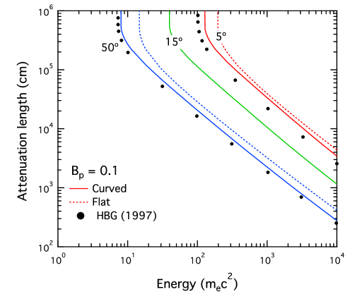
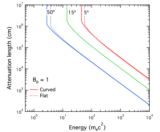
Figure 5.— Attenuation lengths for photons emitted at colatitudes of 5, 15, and 50 degrees, as functions of the photon energy $\,\varepsilon\,$ that is observed at infinity, for a neutron star with surface polar magnetic field of $\,B_{p}=0.1\,$ (left) and $\,B_{p}=1\,$ (right). These represent the quantity $\,L\,$, defined in Eq. (46) for curved spacetime (solid curves) and Eq. (7) for flat spacetime (dotted lines). All curves use the threshold-corrected attenuation coefficient in Eq. (3). The curves turn up and asymptotically approach infinity at the escape energy $\,\varepsilon_{\rm esc}\,$. The large dots for the $\,B_{p}=0.1\,$ case on the left depict pair attenuation lengths from Fig. 2 of Harding, Baring & Gonthier (1997), specifically for emission colatitudes $\,\theta_{\hbox{\sixrm E}}\,$ of $\,5^{\circ}\,$ and $\,50^{\circ}\,$.

Figure 5 displays the attenuation lengths computed for curved spacetime at two different magnetic fields. These are evaluated specifically for emission from the neutron star surface. The curves are monotonically declining functions of photon energy $\,\varepsilon\,$ as observed at infinity. At high energies, where $\,L\ll R_{\hbox{\sixrm NS}}\,$, pair attenuation occurs very close to the surface and general relativistic effects modify the field structure and photon trajectory and redshift in a manner that is essentially independent of $\,\varepsilon\,$. Accordingly, for the $\,B=0.1\,$ example, a dependence $\,L\propto(\varepsilon\theta_{\hbox{\sixrm E}})^{-1}\,$ is approximately realized, just like the Minkowski spacetime dependence deduced from Eq. (30), but with a smaller coefficient of proportionality in the GR case. The influence of curved spacetime reduces $\,L\,$ slightly, primarily because it amplifies both the field strength and the photon energy in the LIF. In the $\,B=1\,$ example, the GR-corrected and flat spacetime attenuation lengths are almost identical because photon conversion arises very soon after pair threshold ($\omega_{\perp}=2$) in the LIF is crossed during propagation. The trajectories then sample regimes $\,\Psi_{\hbox{\sixrm E}}\ll\Psi_{b}\,$ before attenuation, so that the path length differential in Eq. (44) approximately satisfies $\,ds/dr\approx 1/\sqrt{1-\Psi_{\hbox{\sixrm E}}}\,$, using $\,dr/r=-d\Psi/\Psi\,$. Hence the post-Newtonian GR correction to the path length $\,s=L\,$ is precisely that for the blueshift of the photon energy in the LIF. Accordingly, the computation of $\,L\,$ in such threshold-conversion domains is insensitive to general relativistic modifications.

At low energies, the curves turn up and asymptotically approach infinity at the escape energy $\,\varepsilon_{\rm esc}\,$. A small shift in escape energy is evident, due largely to the gravitational redshifting of the photon energy. The monotonic trend of decreasing $\,L\,$ and $\,\varepsilon_{\rm esc}\,$ with increasing colatitude $\,\theta_{\hbox{\sixrm E}}\,$ of emission is a result of increased field line curvature away from the magnetic polar regions. The footpoint emission colatitude $\,\theta_{f}\equiv\theta_{\hbox{\sixrm E}}\,$ can be coupled to a pulsar rotation period if it is assumed to be applicable to the last open field line, $\,\theta_{f}\to\theta_{p}\,$. For a dipolar field in flat space-time this “polar cap” colatitude is given by $\,\sin^{2}\theta_{p}=2\pi R_{\hbox{\sixrm NS}}/(Pc)\equiv R_{\hbox{\sixrm NS}}/R_{\hbox{\sixrm LC}}\,$, where $\,R_{\hbox{\sixrm LC}}=Pc/2\pi\,$ is the light cylinder radius. With general relativistic modifications to the field structure, as defined by Eq. (34),

$$\sin^{2}\theta_{p}\;=\;\hbox{${{\displaystyle\Psi_{\hbox{\sixrm LC}}\,\xi_{r}(\Psi_{\hbox{\sixrm LC}})\vphantom{(}}\over{\displaystyle\Psi_{\hbox{\sixrm E}}\,\xi_{r}(\Psi_{\hbox{\sixrm E}})\vphantom{(}}}$}\quad.$$ (47)

This is Eq. (27) of Gonthier & Harding (1994). Here $\,\Psi_{\hbox{\sixrm LC}}=r_{s}/R_{\hbox{\sixrm LC}}\,$, which is usually much less than unity for young pulsars, so that $\,\xi_{r}(\Psi_{\hbox{\sixrm LC}})\approx 1/3\,$. Generally, $\,\Psi_{\hbox{\sixrm E}}=r_{s}/R_{\hbox{\sixrm NS}}\,$ is not much less than unity. Finally, for the $\,B_{p}=0.1\,$ case (left panel), Fig. 5 also displays points corresponding to the pair attenuation computations in Fig. 2 of Harding, Baring & Gonthier (1997). Our $\,L\,$ results here range from 10–30% higher than these older evaluations — this difference is discussed below.

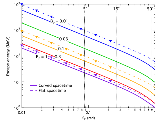
Figure 6.— Escape energies from the neutron star surface in curved spacetime for the attenuation rate defined in Eq. (46). The dashed curves are taken from the solid lines in Fig. 3 and represent the flat spacetime escape energies for the same magnetic fields. Triangles are the escape energies calculated by Chang, Chen, & Ho (1996), as in Fig. 3. Colatitudes of 5, 15, and 50 degrees are marked for easier comparison with Fig. 5. Including GR effects lowers the escape energies, but preserves the same slope because the basic form of the exponential in the attenuation coefficient is unchanged.

The escape energies calculated for the general relativistic analysis are shown in Fig. 6, as functions of the emission colatitude, for different polar magnetic field strengths. Also depicted are the flat space-time equivalents for $\,B_{p}=0.01,0.1,1\,$ (in units of $\,B_{\rm cr}\,$), clearly demonstrating that GR corrections have a greater impact for $\,B_{p}\ll 1\,$ cases (almost by a factor of two) than for $\,B_{p}\approx 1\,$ domains. When $\,\theta_{\hbox{\sixrm E}}\ll 1\,$, the escape energies for curved spacetime simply satisfy $\,\varepsilon_{\rm esc}\propto\theta_{\hbox{\sixrm E}}^{-1}\,$, as expected, since the form of the argument of the exponential in the pair creation attenuation coefficient remains approximately the same as for the flat space-time situation: photon conversion arises well above pair threshold. In this low emission colatitude regime ($\,\theta_{\hbox{\sixrm E}}\lesssim 0.2\,$), when the field is highly sub-critical, it then also follows that $\,\varepsilon_{\rm esc}\propto B_{p}^{-1}\,$, a dependence that is evident in the Figure. Once the polar field approaches and exceeds $\,B_{\rm cr}\,$, the escape energies become almost independent of the field value, because any pair conversion at high altitudes still is fairly near the threshold $\,\omega_{\perp}=2\,$.

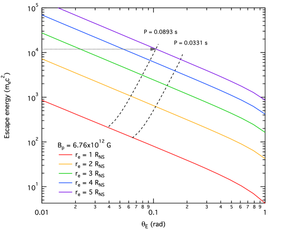
Figure 7.— Pair creation escape energies in curved spacetime for five altitudes of emission, as a function of emission colatitude. The unscaled surface polar magnetic field $\,B_{p}=6.76\times 10^{12}\,$Gauss is that for the Vela pulsar, and is only slightly different from the value for the Crab pulsar. The two dotted curves represent the loci of colatitudes appropriate for the last open field line for pulsars with periods of 0.033 s (Crab) and 0.089 s (Vela). Also marked with the horizontal arrow is twice the cutoff energy $\,E_{c}=3.03\,$GeV measured in the Fermi-LAT phase-averaged spectrum of Vela, identifying the minimum altitude of $\,r_{\hbox{\sixrm E}}\approx 5R_{\hbox{\sixrm NS}}\,$ for super-GeV emission in this pulsar.

In Fig. 7, the general relativistic escape energy is again plotted as a function of emission colatitude, but now illustrating the dependence upon emission altitude $\,r_{\hbox{\sixrm E}}=hR_{\hbox{\sixrm NS}}\,$. This evinces the expected increase of $\,\varepsilon_{\rm esc}\,$ as the emission point becomes more remote from the stellar surface. To forge a preliminary connection with pulsar observations, contours in this escape energy phase space are depicted for the last open field lines pertinent to the Crab and Vela pulsars. These employ solutions of Eq. (47) for the parametric locus of this field lines, specifically for the two different pulsar periods, and curve somewhat down near the stellar surface since curved space-time reduces the polar cap size (e.g. see GH94). At low altitudes, the trend of $\,\varepsilon_{\rm esc}\propto h^{2}\,$ is approximately realized along these diagonal contours. Once the emission altitude rises above $\,h\gtrsim 2\,$, GR influences are quite small, and the flat spacetime trend of $\,\varepsilon_{\rm esc}\propto h^{5/2}\,$ in Eq. (18) is approximately satisfied instead along these contours. The reduction of the polar cap size is primarily responsible for the general relativistic weakening of the altitude dependence near the stellar surface. To find a minimum altitude for emission, one locates the point on these contours of constant period where $\,\varepsilon_{\rm esc}=\alpha E_{c}\,$, where $\,\alpha=2\,$ and $\,E_{c}\,$ is the exponential cutoff energy of the observed pulsar spectrum. The choice for the Vela pulsar, where $\,E_{c}=3.03\,$GeV for the phase-averaged spectrum (Abdo et al., 2013), is illustrated in the upper left, yielding an estimate for the minimum altitude of emission $\,r_{\rm min}\approx 5R_{\hbox{\sixrm NS}}\,$ for Vela. This bound delineates the range of altitudes for which pair transparency is achieved in the magnetosphere of a given pulsar, for emission along the last open field line. This protocol for constraining the emission zones of pulsars is discussed at greater length in Section. 6.

The pair production attenuation lengths and escape energies computed here differ slightly from those presented in Harding, Baring & Gonthier (1997) and Baring & Harding (2001). The attenuation lengths in Fig. 5 are systematically higher by around 10% than those in the left panel of Fig. 2 of Harding, Baring & Gonthier (1997). The escape energies in Fig. 6 are higher than the corresponding evaluations in Harding, Baring & Gonthier (1997) by around 20-30%. The origin of this difference is presently unclear. We observe that there appears to be a slight disagreement between the values of $\,\sin\theta_{\hbox{\sevenrm kB}}\,$ computed in Harding, Baring & Gonthier (1997) for curved spacetime and those derived in this work and in Gonthier & Harding (1994), with those in Harding, Baring & Gonthier (1997) being about 15–20% higher. This is consistent with the slightly lower values of $\,L\,$ and $\,\varepsilon_{\rm esc}\,$ computed in Harding, Baring & Gonthier (1997) relative to those here. As noted above, there is excellent agreement between our geometry and attenuation coefficient calculations and those presented in Gonthier & Harding (1994). Our numerical results for the GR case map continuously over to the $\,\Psi_{\hbox{\sixrm E}}\to 0\,$ flat spacetime cases illustrated in Sec. 3. These latter checks indicate that the curved spacetime results presented here appear to be robust.

As a concluding focus, the techniques in this Section can be applied to downward-traveling photons as well, a consideration that is germane to determining polar cap and surface reheating. A curvature photon emitted from an inward-bound electron or positron will experience both stronger magnetic fields and larger $\,\sin\theta_{\hbox{\sevenrm kB}}\,$ along its path than its outward-traveling counterpart, so its escape energy will be considerably lower. Fig. 8 shows the escape energies for photons emitted along the last open field line in curved spacetime. Solid curves represent upward-traveling photons; dashed curves represent downward-traveling photons. The dashed curves come to an end where photons emitted from the altitude on the x-axis would impact the neutron star. The different colored curves represent parameters for three different pulsars: Crab (red), B1509-58 (J1513-5908; blue), and Geminga (purple).

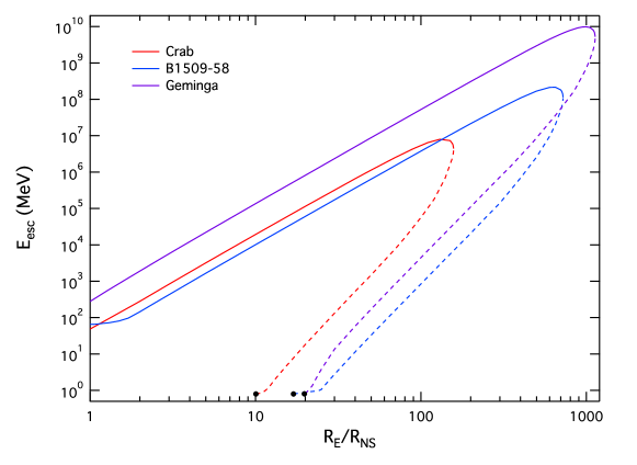
Figure 8.— Escape energies in MeV for photons emitted parallel to the last open field line for pulsars with periods and surface magnetic field strengths equal to those of three observed pulsars. Solid curves indicate a photon traveling in the direction of increasing colatitude ($\,\eta>0\,$, the “upward” direction). Dashed curves indicate a photon traveling in the direction of decreasing colatitude ($\,\eta<0\,$ with $\,\eta\,$ defined as in Fig. 1, the “downward” direction). General relativistic effects are included in this analysis, but rotational aberration effects are not. The dashed curves come to an end (black dots) where photons emitted from the altitude on the x-axis would impact the neutron star. Note that the escape energy at this point may be less than the pair creation threshold of $\,2m_{e}c^{2}\,$ because the energy at infinity will be blueshifted above the threshold close to the neutron star.

The downward-traveling curves come to an end when the emission location starts to experience the neutron star’s shadow. The edge of the shadow can by found by solving for the maximum $\,\Psi\,$ (corresponding to the distance of closest approach to the neutron star) for a photon trajectory, and then setting that maximum $\,\Psi\,$ equal to $\,2M/R\,$ and solving for the emission radius. Using Gonthier & Harding (1994) Eq. (10) (recast in our preferred variables), we can find the maximum $\,\Psi\,$ by solving the cubic equation in $\,\Psi\,$ given by

$$0\;=\;\left(\frac{d\Psi}{d\theta}\right)^{2}\equiv\Psi_{b}^{2}-\Psi^{2}\left(1-\Psi\right)\quad.$$ (48)

$\,\Psi_{b}\,$ depends only on the emission location, so using Eq. (37) and Gonthier & Harding (1994) Eq. (27) to get $\,\Psi_{b}(h)\,$ for emission along the last open field line, we can find $\,\Psi_{\rm max}(h)\,$. When the trajectory just clips the neutron star, we will have

$$\Psi_{\rm max}(h)\;=\;\frac{2M}{R}\quad,$$ (49)

and this can be numerically solved for $\,h\,$ to give the intersection of the edge of the shadow and the last open field line. The escape energy for the trajectory that passes closest to the neutron star can also be estimated. This surface-skimming path passes through the region where the magnetic field is strongest and $\,\sin\theta_{kB}\,$ is close to 1, so the attenuation rate will be very large. For all the pulsars shown here, the absolute pair creation threshold of $\,\omega=2m_{e}c^{2}\,$ acts as a wall in this region. The photons will pair-produce as soon as their energy (gravitationally blueshifted in the local inertial frame) is above threshold, so the energy at infinity for photons that can escape from the edge of the shadow is given approximately by

$$\varepsilon\;\approx\;2\sqrt{1-\Psi_{\rm max}}=1.513\,$$ (50)

(in units of $\,m_{e}c^{2}\,$) for $\,M=1.44M_{\odot}\,$, $\,R=10^{6}\rm{cm}\,$. This is independent of $\,h\,$, which is determined using the above protocol. Threshold effects are stronger in pulsars with stronger magnetic fields, as we showed in Section 3.2, and we can see that for the high-field pulsar B1509-58, both the upward-traveling and downward-traveling curves begin to flatten out at the lower ends where the photons pass closest to the neutron star. A more extreme example of this can be seen in the magnetar case in Fig. 13, where the magnetic field is supercritical and the pair creation threshold strongly influences escape energies up to high altitudes.

For emission points at small to moderate fractions of the light cylinder radius, the escape energies for upward-traveling photons show a power law dependence on emission altitude with an index of approximately $\,5/2\,$. This is expected since general relativistic effects will become negligible very quickly as we move away from the surface and Eq. (18) applies. Calculating the expected power law index for the downward-traveling curves is more difficult, since none of the small-angle approximations we used to obtain Eq. (18) are valid at $\,\Psi=\Psi_{\rm max}\,$, which is where pair attenuation is anticipated to be most effective. Then GR contributions cannot be neglected when the photon passes close to the neutron star even if it was emitted at a high altitude. However, we can make a naive flat spacetime estimate by solving for the value of $\,\eta\,$ at the point of closest approach to the neutron star and performing a series expansion of the argument of the exponential in Eq. (2) at that point. If we set the argument of the exponential equal to 1, we can then solve for $\,\omega\,$ in terms of $\,h\,$. This analysis suggests a leading order contribution of $\,\varepsilon_{\rm esc}\propto h^{4}\,$, with a non-negligible $\,h^{5}\,$ term as well. This is not too divergent from the actual approximate power law dependence of $\,\omega\propto h^{9/2}\,$.

A few global characteristics are easily discerned from this analysis. First, downward-traveling photons are attenuated much more strongly than upward-traveling photons, with escape energies orders of magnitude lower than their outbound counterparts for the same emission location. Second, even with the stronger attenuation, photons emitted in the downward direction from high altitude gaps may still be visible in the Fermi-LAT band if they are not attenuated by other means such as via $\,\gamma\gamma\to e^{+}e^{-}\,$ pair creation. For the Crab pulsar parameters, for example, downward-traveling 300 MeV photons emitted from a gap along the last open field line can escape to infinity if they originate above approximately 40 neutron star radii.

5. RELATIVISTIC ABERRATION DUE TO STELLAR ROTATION

In a pulsar’s rapidly rotating magnetosphere, the attenuation rate due to magnetic pair creation is affected by the deformation of the magnetic field lines, both at high altitudes where the corotation velocity is a significant fraction of the speed of light and at low altitudes near the magnetic pole. This phenomenon can equivalently be described as the aberration of the photon momentum and energy from the rotating stellar field frame. Since pair opacity considerations are focused primarily on the inner magnetosphere, it is the polar zone that is of principal interest in this Section. The computation here for the optical depth is first derived for the most general case of arbitrary emission colatitudes and altitudes in an oblique rotating neutron star, and then restricted to special cases where one can derive incisive analytic approximations. In these calculations, we consider only a rotating rigid dipole field and neglect effects near the pole caused by sweepback of field lines near the light cylinder (e.g. Dyks & Harding, 2004). We will also neglect general relativity effects, which have already been explored extensively.

Our overall approach will be to calculate the photon’s straight-line trajectory in the inertial observer frame (denoted throughout by the subscript “O”), transform it into the magnetic field rest frame (an instantaneous non-inertial frame denoted by subscript “S” for “star frame”) where it is a curved path, and therein calculate the instantaneous photon momentum and magnetic field at every point along this path. This then yields a straightforward determination of the angle $\,\sin\theta_{\hbox{\sevenrm kB}}\,$ from the magnitude of the cross product of the magnetic field and trajectory vectors. Since the characteristics of the rate under Lorentz boosts along the magnetic field are captured in the form in Eq. (1), with the explicit appearance of the Lorentz invariant $\,\omega_{\rm s}\sin\theta_{\hbox{\sevenrm kB}}\,$, this completely leads to the specification of the reaction rate in the star frame. To return to the observer frame, note that Eq. (23) of Daugherty & Harding (1983) (see also Daugherty & Lerche, 1975b) provides a general transformation law for calculating the attenuation rate in a non-inertial rotating frame, given the rate in the inertial observer frame in which both magnetic and rotation-induced electric fields are present. One can invert this by interchanging the roles of the two frames, noting that in the rotating star frame, there is no electric field and thus the $\,\mathbf{E}\times\mathbf{B}\,$ drift velocity is zero. The attenuation rate in the observer frame $\,R^{\rm pp}_{\hbox{\sixrm O}}\,$ is then just the rate calculated in the rotating frame $\,R^{\rm pp}_{\hbox{\sixrm S}}\,$, modified by a time dilation factor of $\,1/\gamma\,$ for the boost between the two frames, i.e. $\,R^{\rm pp}_{\hbox{\sixrm O}}=R^{\rm pp}_{\hbox{\sixrm S}}/\gamma\,$. While the boost depends on the location of the photon along its path to escape, this protocol is algorithmically simple: it avoids accounting for the complex time development of a sequence of Lorentz boosts between trajectory points in the non-inertial star frame.

The instantaneous attenuation rate in the rest frame of an inertial observer employed in this Section is given by the Erber form, and following Eqs. (6) and (8) of Daugherty & Lerche (1975b) is

$$R^{\rm pp}_{\hbox{\sixrm O}}\;\approx\;\frac{1}{\gamma}\frac{3\sqrt{3}}{16\sqrt{2}}\frac{\alpha_{f}}{\lambda\hbox to0.0pt{\hss--}}B\sin\theta_{\hbox{\sevenrm kB}}\exp\left[-\frac{8}{3\omega_{\hbox{\sixrm S}}B\sin\theta_{\hbox{\sevenrm kB}}}\right]\quad.$$ (51)

Here $\,\gamma=1/\sqrt{1-\beta^{2}}\,$ is the Lorentz factor corresponding to the local corotation velocity $\,\beta=v/c\,$ and $\,\omega_{\hbox{\sixrm S}}\,$ is the photon energy in the star frame. As before, $\,\sin\theta_{\hbox{\sevenrm kB}}\,$ is the angle between the photon propagation direction and the local magnetic field direction in the rotating frame, given by

$$\sin\theta_{\hbox{\sevenrm kB}}\;=\;\Bigl{|}\mathbf{\hat{k}_{S}}\times\mathbf{\hat{B}_{S}}\Bigr{|}\quad.$$ (52)

$\,\mathbf{\hat{B}_{S}}\,$ and $\,\mathbf{\hat{k}_{S}}\,$ are, respectively, the magnetic field direction vector and the direction of photon travel in the rotating frame. It is generally straightforward to substitute the threshold-corrected approximate rate from Baier & Katkov (2007) given in Eq. (3), but here we will not do so except for illustrative purposes in Figure 10. The Erber rate gives an accurate description of the character of the results when the magnetic field is significantly subcritical, as it is for most very short-period pulsars. More importantly, its simpler mathematical form is more amenable to the analytic approximations developed in this Section. Corrections imposed by using the BK07 rate will be small in most cases, and the direction of the changes will be exactly as expected from Section 3.2: escape energies will increase by a factor that is an increasing function of the surface polar magnetic field.

Figure 9.— Geometry definitions for photon emission from the magnetosphere of a rotating neutron star. The angle $\,\alpha_{i}\,$ between the rotation axis $\,\mathbf{\Omega}\,$ and the magnetic axis $\,\boldsymbol{\mu}\,$ is the pulsar inclination angle. The coordinates $\,\theta_{\hbox{\sixrm E}}\,$ and $\,\phi_{\hbox{\sixrm E}}\,$, the colatitude and azimuthal angle of the point of emission, are defined with respect to the magnetic axis. Light blue curved lines are magnetic field lines. The vectors $\,\boldsymbol{\beta_{\hbox{\sixrm E}}}\,$ and $\,\mathbf{k_{O}}\,$ are the scaled velocity and photon trajectory in the observer frame at the point of emission; $\,\boldsymbol{\beta_{\hbox{\sixrm E}}}\,$ is directed into the page and $\,\mathbf{k_{O}}\,$ is directed out of the page. Though it is not easily discernable in this diagram, $\,\mathbf{k_{O}}\,$ is not exactly tangent to the magnetic field line that passes through the emission point, but tilted slightly away from the velocity vector.

The geometry for the photon emission and opacity determination is illustrated in Fig. 9, where the magnetic dipole axis is inclined at an angle $\,\alpha_{i}\,$ relative to the spin axis. In Cartesian coordinates with the $\,z\,$ axis aligned with the rotation axis and the $\,xz\,$ plane defined as that containing the magnetic and rotation axes (so that for an orthogonal rotator with $\,\alpha_{i}=90^{\circ}\,$, the magnetic axis is aligned with the $\,+x\,$ axis), the magnetic field (light blue lines in the Figure) at observer time $\,t_{\hbox{\sixrm O}}=0\,$ is given by

$$\mathbf{B_{S}}(0)\;=\;\begin{bmatrix}B_{x}(0)\\ B_{y}(0)\\ B_{z}(0)\end{bmatrix}\;=\;\frac{3B_{p}R_{\hbox{\sixrm NS}}^{3}}{2r_{\hbox{\sixrm S}}^{3}}\begin{bmatrix}\cos\alpha_{i}\cos\theta_{\hbox{\sixrm S}}\sin\theta_{\hbox{\sixrm S}}\cos\phi_{\hbox{\sixrm S}}+\sin\alpha_{i}\left(\cos^{2}\theta_{\hbox{\sixrm S}}-\frac{1}{3}\right)\\ \cos\theta_{\hbox{\sixrm S}}\sin\theta_{\hbox{\sixrm S}}\sin\phi_{\hbox{\sixrm S}}\\ -\sin\alpha_{i}\cos\theta_{\hbox{\sixrm S}}\sin\theta_{\hbox{\sixrm S}}\cos\phi_{\hbox{\sixrm S}}+\cos\alpha_{i}\left(\cos^{2}\theta_{\hbox{\sixrm S}}-\frac{1}{3}\right)\end{bmatrix}.$$ (53)

By specifying a standard dipole $\,\mu_{\hbox{\sixrm B}}(3\cos\theta_{\hbox{\sixrm S}}\sin\theta_{\hbox{\sixrm S}},\,0,\,3\cos^{2}\theta_{\hbox{\sixrm S}}-1)/r_{s}^{3}\,$, where $\,\mu_{\hbox{\sixrm B}}=B_{p}R_{\hbox{\sixrm NS}}^{3}/2\,$ is the dipole moment, this form is simply obtained by performing sequential rotations by $\,\phi_{\hbox{\sixrm S}}\,$ about the $\,z\,$-axis and then $\,\alpha_{i}\,$ about the $\,y\,$-axis, the latter of which can be described by the rotation matrix (subscript I denotes the magnetic inclination operator)

$$T_{\rm I}\;=\;\begin{bmatrix}\cos\alpha_{i}&0&\sin\alpha_{i}\\ 0&1&0\\ -\sin\alpha_{i}&0&\cos\alpha_{i}\end{bmatrix}\quad.$$ (54)

Throughout this presentation, the subscript S denotes quantities in the star frame, and the angles in Eq. (53) relate to spherical polar coordinates in that frame. To derive the time development of this field $\,\mathbf{B_{S}}(t_{\hbox{\sixrm O}})\,$ as the star rotates about the $\,z\,$ axis while a photon escapes the magnetosphere, we multiply this by the appropriate rotation matrix $\,\mathbf{T}_{\Omega}\,$:

$$\mathbf{B_{S}}(t_{\hbox{\sixrm O}})\;=\;\mathbf{T}_{\Omega}\cdot\mathbf{B_{S}}(0)\quad,\quad\mathbf{T}_{\Omega}(t_{\hbox{\sixrm O}})\;=\;\begin{bmatrix}\cos\Omega t_{\hbox{\sixrm O}}&-\sin\Omega t_{\hbox{\sixrm O}}&0\\ \sin\Omega t_{\hbox{\sixrm O}}&\cos\Omega t_{\hbox{\sixrm O}}&0\\ 0&0&1\end{bmatrix}\quad.$$ (55)

Here $\,t_{\hbox{\sixrm O}}=s/c\,$ is the time an observer determines as the photon propagates a distance $\,s\,$ after emission. In general, $\,\Omega t_{\hbox{\sixrm O}}\ll 1\,$ for the low altitude propagation zones where the greatest contributions to pair opacity are realized. It is important to note that $\,\mathbf{B_{S}}\,$ represents the field vector in the instantaneous star frame at time $\,t_{\hbox{\sixrm O}}\,$, and must be boosted to the observer frame to define the complete electromagnetic field therein.

For initial conditions, it is assumed that the photon is emitted very nearly parallel to the magnetic field at the point of emission in the star frame, as was done for the non-rotating case. The spherical polar coordinates at this point are $\,r_{\hbox{\sixrm S}}=r_{\hbox{\sixrm E}}\,$, $\,\theta_{\hbox{\sixrm S}}=\theta_{\hbox{\sixrm E}}\,$, and $\,\phi_{\hbox{\sixrm S}}=\phi_{\hbox{\sixrm E}}\,$, as depicted in Figure 9. Normalizing this vector gives the direction of the magnetic field, which depends only on the colatitude and azimuthal angle, and can be obtained directly from Eq. (53). In the inertial observer (O) frame, the magnetic field direction vector and the photon trajectory vector will no longer be parallel at the point of emission, due to relativistic aberration precipitated by the rotation. To specify this, the corotation velocity $\,\overrightarrow{\beta_{\hbox{\sixrm E}}}c\,$ at the point of emission is needed. This depends only on the pulsar period and the 3D location of the emission point, and is given by

$$\overrightarrow{\beta_{\hbox{\sixrm E}}}\;=\;\frac{2\pi r_{\hbox{\sixrm E}}}{cP}\begin{bmatrix}-\sin\theta_{\hbox{\sixrm E}}\sin\phi_{\hbox{\sixrm E}}\\ \cos\alpha_{i}\sin\theta_{\hbox{\sixrm E}}\cos\phi_{\hbox{\sixrm E}}+\sin\alpha_{i}\cos\theta_{\hbox{\sixrm E}}\\ 0\end{bmatrix}\quad.$$ (56)

For $\,r_{\hbox{\sixrm E}}\leq Pc/2\pi\,$ this dimensionless speed is always less than unity, except in the special case of emission at the equatorial light cylinder radius ($\,\theta_{\hbox{\sixrm E}}=\pi/2\,$, $\,r_{\hbox{\sixrm E}}=Pc/2\pi\,$) and for an aligned rotator ($\,\alpha_{i}=0\,$).

We now progress to the construction of the photon’s path in the reference frame of an inertial observer, which is a straight line in the absence of general relativistic corrections. Using the photon’s starting direction in the star frame, labelled by the unit vector $\,\mathbf{\hat{k}_{S,E}}\equiv\mathbf{\hat{B}_{S,E}}\,$ derived from Eq. (53), and the instantaneous relative velocity between the star frame and the observer frame of $\,\overrightarrow{\beta_{\hbox{\sixrm E}}}c\,$, we can calculate the photon’s trajectory vector in the observer frame by performing a Lorentz transformation on the photon’s 4-momentum in the star frame:

$$\mathbf{k_{O}}\;=\;\omega_{\hbox{\sixrm S,E}}\left\{\mathbf{\hat{B}_{S,E}}+\gamma_{\hbox{\sixrm E}}\left[\frac{\gamma_{\hbox{\sixrm E}}}{\gamma_{\hbox{\sixrm E}}+1}\left(\overrightarrow{\beta_{\hbox{\sixrm E}}}\cdot\mathbf{\hat{B}_{S,E}}\right)-1\right]\overrightarrow{\beta_{\hbox{\sixrm E}}}\right\}\quad.$$ (57)

Following the dimensionless convention adopted throughout, the wave vector $\,\mathbf{k_{O}}\,$ is scaled in terms of the inverse Compton wavelength $\,m_{e}c/\hbar\,$, as is its star frame counterpart $\,\mathbf{k_{S}}\,$ below. In the star frame, the photon energy at the point of emission, $\,\omega_{\hbox{\sixrm S,E}}\,$, is Doppler-shifted relative to the constant photon energy $\,{\varepsilon_{\hbox{\sixrm O}}}\,$ in the inertial observer frame:

$$\omega_{\hbox{\sixrm S,E}}\;=\;\hbox{${{\displaystyle\varepsilon_{\hbox{\sixrm O}}\vphantom{(}}\over{\displaystyle\gamma_{\hbox{\sixrm E}}\,\bigl{(}1-\mathbf{\hat{B}_{S,E}}\cdot\overrightarrow{\beta_{\hbox{\sixrm E}}}\bigr{)}\vphantom{(}}}$}\quad.$$ (58)

This completes the specification of $\,\mathbf{k_{O}}\,$, which is a constant during propagation to infinity. When $\,\beta_{\hbox{\sixrm E}}\,$ is small, as it is for emission relatively close to the neutron star, all quantities that are second order in $\,\beta_{\hbox{\sixrm E}}\,$ can be neglected, so that Eq. (57) approximately assumes the form

$$\mathbf{k_{O}}\;\approx\;\varepsilon_{\hbox{\sixrm O}}\left\{\mathbf{\hat{B}_{S,E}}-\overrightarrow{\beta_{\hbox{\sixrm E}}}\right\}\quad.$$ (59)

The small-$\,\beta\,$ approximation will be considered in more detail later in this Section and also in Appendix B, for the purposes of generating useful analytic developments.

To compute the reaction rates in Eq. (51), one needs the direction of photon travel in the star frame, where the path is curved, so that the value of $\,\sin\theta_{\hbox{\sevenrm kB}}\,$ can be determined. This direction can be obtained at each point by transforming $\,\mathbf{k_{O}}\,$ back to the star frame, using the instantaneous $\,\beta\,$ and $\,\gamma\,$ at each point. This transformation preserves the component of momentum $\,\mathbf{k_{\perp}}=\mathbf{k_{O}}-\bigl{(}\mathbf{k_{O}}\cdot\hat{\beta}\bigr{)}\,\hat{\beta}\,$ orthogonal to the boost, but stretches/contracts the component along $\,\vec{\beta}\,$ via the relation $\,\mathbf{k_{S}}\cdot\hat{\beta}=\gamma\bigl{(}\mathbf{k_{O}}\cdot\hat{\beta}+\beta\,|\mathbf{k_{O}}|\,\bigr{)}\,$, similar to the protocol adopted for Eq. (57). The momentum vectors of the photon in the two frames at each position along the trajectory are then given by the conjugate relations

$$\mathbf{k_{O}} = \mathbf{k_{S}}+\gamma\left[\frac{\gamma}{\gamma+1}\left(\overrightarrow{\beta}\cdot\mathbf{k_{S}}\right)-|\mathbf{k_{S}}|\right]\overrightarrow{\beta}\quad,$$

$$\mathbf{k_{S}} = \mathbf{k_{O}}+\gamma\left[\frac{\gamma}{\gamma+1}\left(\overrightarrow{\beta}\cdot\mathbf{k_{O}}\right)+|\mathbf{k_{O}}|\right]\overrightarrow{\beta}\quad.$$

The first equation in this couplet is just an extension of Eq. (57) to arbitrary altitudes using $\,\overrightarrow{\beta_{\hbox{\sixrm E}}}\to\overrightarrow{\beta}\,$ and $\,\omega_{\hbox{\sixrm S,E}}\mathbf{\hat{B}_{S,E}}\to\mathbf{k_{S}}\,$. To maintain constancy of $\,\mathbf{k_{O}}\,$ along the entire trajectory, $\,|\mathbf{k_{S}}|=\omega_{\hbox{\sixrm S}}\,$ adjusts its value at each point via the aberration relation $\,\gamma\omega_{\hbox{\sixrm S}}\bigl{(}1-\mathbf{\hat{k}_{S}}\cdot\overrightarrow{\beta}\bigr{)}=\varepsilon_{\hbox{\sixrm O}}\,$ that is the analog of Eq. (58). The second relation of this pair is just the inversion of the first, under the interchange S$\,\leftrightarrow\,$O and also $\,\overrightarrow{\beta}\to-\overrightarrow{\beta}\,$; it is that desired for the computation of $\,\sin\theta_{\hbox{\sevenrm kB}}\,$. Observe that forming the dot product $\,\omega_{\hbox{\sixrm S}}^{2}=|\mathbf{k_{S}}|^{2}\,$ can be used to derive the inverse aberration relation $\,\omega_{\hbox{\sixrm S}}=\gamma\varepsilon_{\hbox{\sixrm O}}(1+\mathbf{\hat{k}_{O}}\cdot\overrightarrow{\beta})\,$. Note that in the absence of rotation ($\,P\rightarrow\infty\,$, $\,\beta\rightarrow 0\,$), one recovers $\,\mathbf{k_{S}}=\mathbf{k_{O}}=\varepsilon_{\hbox{\sixrm O}}\mathbf{\hat{B}_{S,E}}\,$, as expected.

Calculating the corotation velocity $\,\overrightarrow{\beta}\,$ at every point along the photon trajectory is straightforward. The straight-line photon path in the observer frame is given simply by

$$\mathbf{r_{O}}=\mathbf{r_{\hbox{\sixrm E}}}+s\mathbf{\hat{k}_{O}},$$ (61)

where $\,s=ct\,$ is the distance traveled, and $\,\mathbf{r_{\hbox{\sixrm E}}}\,$ is the emission point. This is conveniently expressed in spherical coordinates about the rotation axis, still as a function of $\,s\,$:

$$\begin{bmatrix}r_{\hbox{\sixrm O}}(s)\\ \theta_{\hbox{\sixrm O}}(s)\\ \phi_{\hbox{\sixrm O}}(s)\end{bmatrix}\;=\;\begin{bmatrix}\sqrt{r_{\hbox{\sixrm E}}^{2}+s^{2}+2s\mathbf{r_{\hbox{\sixrm E}}}\cdot\mathbf{\hat{k}_{O}}}\;\\ \cos^{-1}\hbox{${{\displaystyle\mathbf{r_{E,z}}+s\mathbf{\hat{k}_{O,z}}\vphantom{(}}\over{\displaystyle r_{\hbox{\sixrm O}}(s)\vphantom{(}}}$}\vphantom{\Biggl{(}}\\ \tan^{-1}\hbox{${{\displaystyle\mathbf{r_{E,y}}+s\mathbf{\hat{k}_{O,y}}\vphantom{(}}\over{\displaystyle\mathbf{r_{E,x}}+s\mathbf{\hat{k}_{O,x}}\vphantom{(}}}$}\end{bmatrix}\quad.$$ (62)

In this form, the coupling between the rotational phase $\,\phi_{\hbox{\sixrm O}}\,$ and the trajectory is simply displayed. In general, we do not restrict the emission plane to zero phase $\,\phi_{\hbox{\sixrm O}}\,$, i.e. $\,\mathbf{k_{O}}\,$, $\,\mathbf{\hat{B}_{S,E}}\,$ and $\,\overrightarrow{\beta_{\hbox{\sixrm E}}}\,$ are not coplanar. The local corotation velocity is then given as a function of $\,s\,$ in Cartesian coordinates by

$$\overrightarrow{\beta}(s)\;=\;\frac{r_{\hbox{\sixrm O}}(s)\Omega}{c}\,\sin\theta_{\hbox{\sixrm O}}\begin{bmatrix}-\sin\phi_{\hbox{\sixrm O}}(s)\\ \cos\phi_{\hbox{\sixrm O}}(s)\\ 0\end{bmatrix}\quad.$$ (63)

Since $\,\mathbf{k_{O}}\,$ in Eq. (57) is also expressible in Cartesian coordinates, the determination of $\,\mathbf{k_{S}}\,$ via Eq. (LABEL:eq:kO_kS_Lorentz_pair) is routine.

The remaining ingredient needed for the determination of the pair conversion rates is the second vector for the calculation of $\,\sin\theta_{\hbox{\sevenrm kB}}\,$ in Eq. (52), namely the magnetic field vector in the star frame, $\,\mathbf{B_{S}}(s)\,$. Given the simple dipolar form in the star frame, the only complexity is encapsulated in the conversion of the straight-line trajectory in the inertial observer frame into star frame coordinates, where the path is curved. Given coordinates $\,\{x_{\hbox{\sixrm O}},y_{\hbox{\sixrm O}},z_{\hbox{\sixrm O}}\}\,$ in the observer frame, obtained from Eq. (61), the photon trajectory in the star frame can be expressed via

$$\begin{bmatrix}ct_{\hbox{\sixrm S}}\\ x_{\hbox{\sixrm S}}\\ y_{\hbox{\sixrm S}}\\ z_{\hbox{\sixrm S}}\end{bmatrix}\;=\;\mathcal{L}\cdot\begin{bmatrix}ct_{\hbox{\sixrm O}}\\ x_{\hbox{\sixrm O}}\\ y_{\hbox{\sixrm O}}\\ z_{\hbox{\sixrm O}}\end{bmatrix}\quad\hbox{for}\quad\mathcal{L}\;=\;\begin{bmatrix}\gamma&\gamma\beta_{x}&\gamma\beta_{y}&0\\ \gamma\beta_{x}&1+\left(\gamma-1\right)\hbox{${{\displaystyle\beta_{x}^{2}\vphantom{(}}\over{\displaystyle\beta^{2}\vphantom{(}}}$}&\left(\gamma-1\right)\hbox{${{\displaystyle\beta_{x}\beta_{y}\vphantom{(}}\over{\displaystyle\beta^{2}\vphantom{(}}}$}&0\\ \gamma\beta_{y}&\left(\gamma-1\right)\hbox{${{\displaystyle\beta_{x}\beta_{y}\vphantom{(}}\over{\displaystyle\beta^{2}\vphantom{(}}}$}&1+\left(\gamma-1\right)\hbox{${{\displaystyle\beta_{y}^{2}\vphantom{(}}\over{\displaystyle\beta^{2}\vphantom{(}}}$}&0\\ 0&0&0&1\end{bmatrix}$$ (64)

being a standard Lorentz transformation matrix, $\,\mathcal{L}=\mathcal{L}(s)\,$. Since the boost is purely in the $\,xy\,$ direction and $\,s=ct_{\hbox{\sixrm O}}\,$, this transformation simplifies to

$$\begin{bmatrix}x_{\hbox{\sixrm S}}\\ y_{\hbox{\sixrm S}}\\ z_{\hbox{\sixrm S}}\end{bmatrix}\;=\;\begin{bmatrix}\gamma\beta_{x}s+\biggl{(}1+\hbox{${{\displaystyle\gamma^{2}\beta_{x}^{2}\vphantom{(}}\over{\displaystyle\gamma+1\vphantom{(}}}$}\biggr{)}x_{\hbox{\sixrm O}}+\hbox{${{\displaystyle\gamma^{2}\beta_{x}\beta_{y}\vphantom{(}}\over{\displaystyle\gamma+1\vphantom{(}}}$}\,y_{\hbox{\sixrm O}}\vphantom{\Biggr{)}}\\ \gamma\beta_{y}s+\hbox{${{\displaystyle\gamma^{2}\beta_{x}\beta_{y}\vphantom{(}}\over{\displaystyle\gamma+1\vphantom{(}}}$}\,x_{\hbox{\sixrm O}}+\biggl{(}1+\hbox{${{\displaystyle\gamma^{2}\beta_{x}^{2}\vphantom{(}}\over{\displaystyle\gamma+1\vphantom{(}}}$}\biggr{)}y_{\hbox{\sixrm O}}\\ z_{\hbox{\sixrm O}}\end{bmatrix}$$ (65)

These Cartesian coordinates are oriented just as in the coordinate configuration at the time $\,t=0\,$ of emission, with the $\,z\,$-axis parallel to $\,\mathbf{\Omega}\,$. The star frame magnetic is most easily specified by defining the polar coordinates in a specification that possesses the current rotational orientation, and is then “de-inclined” with respect to the rotation axis. Since the field configuration has evolved slightly due to the rotation of the star, we sequentially perform inverse rotation and inverse inclination operations

$$r_{\hbox{\sixrm S}}\begin{bmatrix}\sin\theta_{\hbox{\sixrm S}}\cos\phi_{\hbox{\sixrm S}}\\ \sin\theta_{\hbox{\sixrm S}}\sin\phi_{\hbox{\sixrm S}}\\ \cos\theta_{\hbox{\sixrm S}}\end{bmatrix}\;=\;\begin{bmatrix}\overline{x}_{\hbox{\sixrm S}}\\ \overline{y}_{\hbox{\sixrm S}}\\ \overline{z}_{\hbox{\sixrm S}}\end{bmatrix}\;=\;T_{\rm I}^{-1}\cdot T_{\Omega}^{-1}\begin{bmatrix}x_{\hbox{\sixrm S}}\\ y_{\hbox{\sixrm S}}\\ z_{\hbox{\sixrm S}}\end{bmatrix}$$ (66)

to express the star frame Cartesian coordinates in a form that can be directly interpreted for the pertinent spherical polar coordinates — these are now oriented such that $\,\theta_{\hbox{\sixrm S}}=0\,$ corresponds to the magnetic axis, as opposed to the rotation axis. These ($\,r_{\hbox{\sixrm S}},\,\theta_{\hbox{\sixrm S}},\,\phi_{\hbox{\sixrm S}}\,$) coordinates are used to calculate the magnetic field vector $\,\mathbf{B_{S}}\,$ using Eq. (53), which incorporates the inclination element. However, in addition, the time evolution operator $\,T_{\Omega}\,$ must also then be applied, to render the field vector in a form representative of time $\,t_{\hbox{\sixrm O}}\,$, i.e. corresponding to Eq. (55). This protocol then yields $\,\mathbf{B_{S}}\,$ in evolved star frame Cartesian coordinates, which together with Eq. (LABEL:eq:kO_kS_Lorentz_pair) can be employed to routinely evaluate the cross product $\,|\mathbf{k_{S}}\times\mathbf{B_{S}}|\,$, and therefore $\,\sin\theta_{\hbox{\sevenrm kB}}\,$. Coupled with the aberration relation $\,\omega_{\hbox{\sixrm S}}=\gamma\varepsilon_{\hbox{\sixrm O}}(1+\mathbf{\hat{k}_{O}}\cdot\overrightarrow{\beta})\,$, this completes the ensemble of relations need to compute the final rate in Eq. (51).

To obtain the optical depth, we integrate the rate over the path length $\,s\,$. Just as with the non-rotating flat spacetime calculation, it is expedient to change variables from $\,s\,$ to a path angle $\,\eta\,$, defined by

$$s\;=\;\sqrt{r_{\hbox{\sixrm E}}^{2}+r^{2}-2rr_{\hbox{\sixrm E}}\cos\eta}\quad.$$ (67)

This is analogous to that displayed in Fig. 1, but notably with the plane defined by the radius vector and photon momentum at any time being noncoindent with the instantaneous plane containing the magnetic field axis and radial vector at the time of emission. Therefore, Eq. (8) does not apply except when $\,\beta_{\hbox{\sixrm E}}=0\,$ and the star does not rotate, and the general relationship between $\,\eta\,$ and $\,\theta_{\hbox{\sixrm E}}\,$ and $\,\theta\,$ is quite complicated, and contains all the information associated with magnetic field orientation at each rotational phase along the photon’s path to infinity. One advantage of working with this integration variable is that it is always small when $\,\theta_{\hbox{\sixrm E}}\,$ is small, which facilitates an asymptotic analysis (detailed below) that serves to check the computations. Further simplification arises by defining the angle $\,\delta_{\hbox{\sixrm E}}\,$ between the emission and radial directions, just as for the non-rotating flat spacetime analysis, i.e.,

$$\delta_{\hbox{\sixrm E}}\;=\;\cos^{-1}\biggl{(}\hbox{${{\displaystyle\mathbf{r_{\hbox{\sixrm E}}}\cdot\mathbf{\hat{k}_{O}}\vphantom{(}}\over{\displaystyle|r_{\hbox{\sixrm E}}|\vphantom{(}}}$}\biggr{)}\quad.$$ (68)

Then consideration of the appropriate triangles (visualized using Fig. 1) quickly establishes that Eq. (13) applies, so that the optical depth integral becomes

$$\tau_{A}\;=\;r_{\hbox{\sixrm E}}\sin\delta_{\hbox{\sixrm E}}\int_{0}^{\delta_{\hbox{\sixrm E}}}\hbox{${{\displaystyle R_{A}\,d\eta\vphantom{(}}\over{\displaystyle\sin^{2}(\delta_{\hbox{\sixrm E}}-\eta)\vphantom{(}}}$}\quad.$$ (69)

The upper limit of integration is the path angle $\,\eta\,$ when the photon’s trajectory crosses the light cylinder; since this is essentially at infinity, we have $\,\eta_{\hbox{\sevenrm max}}\approx\delta_{\hbox{\sixrm E}}\,$, as in Section 3.

The effects of rotational aberration on the escape energies of photons emitted from the neutron star surface are explored in Fig. 10, specifically as functions of small colatitudes (below around $\,5^{\circ}\,$) near the magnetic pole. The $x$-axis therefore constitutes different locales on the polar cap, with only a select value corresponding to the footpoint of the last open field line i.e., $\,\theta_{\hbox{\sixrm E}}=0.08\,$ ($\,\approx 4.6^{\circ}\,$) for the Crab pulsar. The chosen magnetic field is the Crab value, and most of the results (curves) are generated using the Erber rate. Escape energy curves are generated for three different pulse periods and two different rotator inclinations $\,\alpha_{i}\,$. Results are also displayed for different azimuthal angles $\,\phi_{\hbox{\sixrm E}}\,$, with $\,\phi_{\hbox{\sixrm E}}=0\,$ corresponding to emission points lying in the plane defined by $\,\mathbf{k_{O}}\,$ and $\,\mathbf{\hat{B}_{S,E}}\,$. As $\,\phi_{\hbox{\sixrm E}}\,$ is changed to accommodate different rotational phases, different local rotational speeds $\,\beta_{\hbox{\sixrm E}}\,$ are sampled, with $\,\phi_{\hbox{\sixrm E}}>0\,$ defining cases where the non-radial component of photon momentum is in the direction of rotation, and $\,\phi_{\hbox{\sixrm E}}<0\,$ constituting counter-rotation emission cases. Note that this sign convention is opposite the one used by Lee et al. (2010). The Figure exhibits the obvious trend that as the period is decreased from large values ($\,P=100\,$sec, essentially non-rotating), the aberration modifications to $\,\varepsilon_{\rm esc}\,$ become larger at small colatitudes, and their influence persists to larger colatitude domains. Mostly, but not always, rotation reduces $\,\varepsilon_{\rm esc}\,$ since photons can promptly and more readily propagate across field lines in the star frame; this is best exemplified by the $\,P=10\,$ms case. Note the similarity of the $\,\phi_{\hbox{\sixrm E}}=0\,$ aberration-corrected curves in the Figure to the non-rotating $\,\theta_{kB,0}=0.01\,$ curves for magnetic pair attenuation in Figure 1 of Baring & Harding (2001).

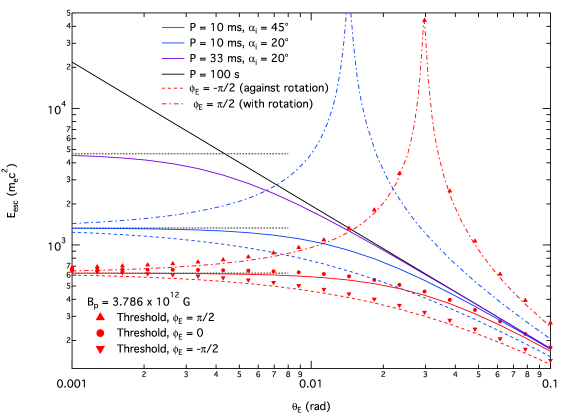
Figure 10.— Escape energies from the neutron star surface for colatitudes near the magnetic pole with three different sets of pulsar parameters, period $\,P\,$, magnetic inclination angle $\,\alpha_{i}\,$, and orbital phase $\,\phi_{\hbox{\sixrm E}}\,$. The magnetic field strength is half the surface polar value for the Crab, and the Erber rate in Eq. (2) is used for the curve computations. The black $\,P=100\,$sec example defines a non-aberration case as discussed in Section 3. Solid curves have an azimuthal angle of $\,\phi_{\hbox{\sixrm E}}=0\,$, where the emission point lies in the plane defined by the magnetic axis and the rotation axis. Dot-dash curves represent emission from an azimuthal angle of $\,\phi_{\hbox{\sixrm E}}=\pi/2\,$, where the photon is emitted with the direction of neutron star rotation. Dashed curves correspond to azimuthal angles of $\,\phi_{\hbox{\sixrm E}}=-\pi/2\,$, against the direction of neutron star rotation. This subdivision into three different azimuthal angle values applies only to $\,P=10\,$ms curves. For the three $\,P=10\,$ms, $\,\alpha_{i}=45^{\circ}\,$ cases, the circles and triangles represent escape energies calculated with the threshold-corrected attenuation rate approximation given in Baier & Katkov (2007). The gray dotted lines represent the small colatitude analytic approximation in Eq. (70) for the 10 ms and 33 ms cases.

At very small colatitudes, the escape energies for the same period and magnetic inclination all approach the same finite value regardless of the initial azimuthal angle about the polar cap. This saturation is a core characteristic of aberration corrections. When the colatitudes are somewhat larger but still fairly small, however, the asymmetry between the leading edge and the trailing edge of the polar cap becomes evident. The trailing edge sees a slight decrease in escape energies caused by the general increase in $\,\sin\theta_{\hbox{\sevenrm kB}}\,$ as the photons’ transit across field lines is aided by the field’s rotation. The leading edge sees an increase of well over an order of magnitude in escape energy, a caustic-like effect that is manifested when the field line sweepback creates a narrow range in colatitudes where the photon’s trajectory is nearly parallel to the magnetic field lines over a substantial section of the photon path. This azimuthal bifurcation of the escape energies is maximized when $\,\theta_{\hbox{\sixrm E}}\sim R_{\hbox{\sixrm NS}}\sin\alpha_{i}/R_{\hbox{\sixrm LC}}\,$, and declines rapidly at larger emission colatitudes. The large value of $\,\varepsilon_{\rm esc}\,$ implies that this constrained portion of the surface polar locale is actually visible in the GeV band that is detected in most Fermi-LAT pulsars. These “leading edge” peaks arise at $\,\theta_{\hbox{\sixrm E}}\approx 2\beta_{p}\,$, where $\,\beta_{p}=R_{\hbox{\sixrm NS}}\sin\alpha_{i}/R_{\hbox{\sixrm LC}}\,$ is the corotational dimensionless speed at the surface magnetic pole, and therefore are proximate to the polar cap of size $\,\theta_{c}\approx\sqrt{R_{\hbox{\sixrm NS}}/R_{\hbox{\sixrm LC}}}\,$. One can therefore infer that a small portion of the polar cap corresponding to a particular phase (i.e., $\,\phi_{\hbox{\sixrm E}}\,$) of pulsation may actually be transparent to pair attenuation up to a few GeV in photon energy.

Also depicted in Fig. 10 are circles, upward-pointing triangles, and downward-pointing triangles, which represent the escape energies calculated with the threshold-corrected rate from Eq. (3) for $\,\phi_{\hbox{\sixrm E}}=0,+\pi/2,-\pi/2\,$ respectively. For this subcritical surface magnetic field, the threshold effects raise the escape energies slightly across the board, but clearly do not alter the general character of the results.

The saturation limiting case of $\,\theta_{\hbox{\sixrm E}}\to 0\,$ is particularly amenable to analytic approximation and should serve as a good indicator of how strongly rotational aberration affects maximum energies and minimum altitudes of emission (addressed below) for magnetic pair creation transparency. For a non-rotating neutron star, a photon emitted from the magnetic pole could never attain a non-zero $\,\sin\theta_{\hbox{\sevenrm kB}}\,$, and so the attenuation rate approaches zero as $\,\theta_{\hbox{\sixrm E}}\rightarrow 0\,$. For a rotating neutron star, the angle between the photon trajectory and the magnetic field at the point of emission is nonzero in the inertial observer frame, even for photons emitted from the magnetic poles. Thus, the attenuation rate is nonzero and minimum emission altitudes and escape energies saturate at meaningful values. Such an asymptotic result can be determined by following a procedure much like the one discussed at some length in Section 3.1. One obtains the following approximation for the optical depth at $\,\theta_{\hbox{\sixrm E}}=0\,$ (with $\,B_{p}\,$ scaled by $\,B_{\rm cr}\,$):

$$\tau_{A}\;\approx\;\hbox{${{\displaystyle 3^{6}\sqrt{3}\vphantom{(}}\over{\displaystyle 2^{18}\vphantom{(}}}$}\hbox{${{\displaystyle\alpha_{f}R_{\hbox{\sixrm NS}}\vphantom{(}}\over{\displaystyle\lambda\hbox to0.0pt{\hss--}\,h^{2}\vphantom{(}}}$}\sqrt{\pi\varepsilon}\,\left(\hbox{${{\displaystyle B_{p}R_{\hbox{\sixrm NS}}\sin\alpha_{i}\vphantom{(}}\over{\displaystyle R_{\hbox{\sixrm LC}}\vphantom{(}}}$}\right)^{3/2}\;\exp\left\{-\hbox{${{\displaystyle 2^{12}h^{2}R_{\hbox{\sixrm LC}}\vphantom{(}}\over{\displaystyle 3^{5}\varepsilon B_{p}\,R_{\hbox{\sixrm NS}}\sin\alpha_{i}\vphantom{\bigl{(}}\vphantom{(}}}$}\right\}\quad,$$ (70)

where $\,h=r_{\hbox{\sixrm E}}/R_{\hbox{\sixrm NS}}\,$, and $\,R_{\hbox{\sixrm LC}}=Pc/2\pi\,$ expresses the pulsar period. The details of this development can be found in Appendix B. Setting this equal to unity, we can solve for $\,\varepsilon_{esc}\,$:

$$\varepsilon_{\rm esc}\;=\;\hbox{${{\displaystyle 2^{12}\,h^{2}\vphantom{(}}\over{\displaystyle 3^{5}\,B_{p}\beta_{p}\vphantom{(}}}$}\left[\log_{e}\hbox{${{\displaystyle\alpha_{f}R_{\hbox{\sixrm NS}}\vphantom{(}}\over{\displaystyle\lambda\hbox to0.0pt{\hss--}\vphantom{(}}}$}+\hbox{${{\displaystyle 1\vphantom{(}}\over{\displaystyle 2\vphantom{(}}}$}\log_{e}\hbox{${{\displaystyle\varepsilon_{\rm esc}\vphantom{(}}\over{\displaystyle h^{4}\vphantom{(}}}$}+\hbox{${{\displaystyle 3\vphantom{(}}\over{\displaystyle 2\vphantom{(}}}$}\log_{e}B_{p}\beta_{p}-5.34\right]^{-1}\quad.$$ (71)

In this expression, $\,\beta_{p}=R_{\hbox{\sixrm NS}}\sin\alpha_{i}/R_{\hbox{\sixrm LC}}\,$ is again the dimensionless rotation speed at the surface polar location in its circular path, and is the key parameter defining the scale of rotational influences. Comparison with the corresponding non-rotating result in Eq. (20) indicates that here $\,\beta_{p}\,$ plays a role equivalent to the footpoint colatitude $\,\theta_{f}\,$ there, because both $\,\beta_{p}\,$ and $\,\theta_{f}\,$ are proportional to the angle between the photon momentum vector and the radial direction at the neutron star surface. Accordingly, aberration modifications should diminish for these low altitude emission considerations when $\,\theta_{\hbox{\sixrm E}}\,$ substantially exceeds $\,\beta_{p}\,$, and all cases should coalesce to the static ($\,P\to\infty\,$), flat spacetime curve: this circumstance is clearly evident in Fig. 10. Observe that the choice of azimuthal angle $\,\phi_{\hbox{\sixrm E}}\,$ provides a second-order correction $\,O(\theta_{\hbox{\sixrm E}}^{2})\,$ when at extremely small colatitudes above the magnetic pole, and so does not appear in these leading-order asymptotic formulae.

The transcendental Eq. (71) must be solved numerically, in general, though the weak dependence on $\,\varepsilon_{\rm esc}\,$ in the logarithmic term, when neglected, permits approximate analytic solution for the escape energy. Numerical results are diplayed as the gray dashed line saturation asymptotes in Fig. 10, for the case of surface emission ($\,h=1\,$) and periods 10 ms and 33 ms. One can immediately see that to leading order, as $\,\theta_{\hbox{\sixrm E}}\to 0\,$, since $\,\varepsilon_{\rm esc}\propto\beta_{p}^{-1}\,$, one should expect to see $\,\varepsilon_{\rm esc}\propto P\,$ and $\,\varepsilon_{\rm esc}\propto 1/\sin\alpha_{i}\,$: these dependences are clearly exhibited in the Figure. Moreover, the computed numerical $\,\varepsilon_{\rm esc}\,$ curves asymptotically approach the solutions of Eq. (71) as $\,\theta_{\hbox{\sixrm E}}\to 0\,$.

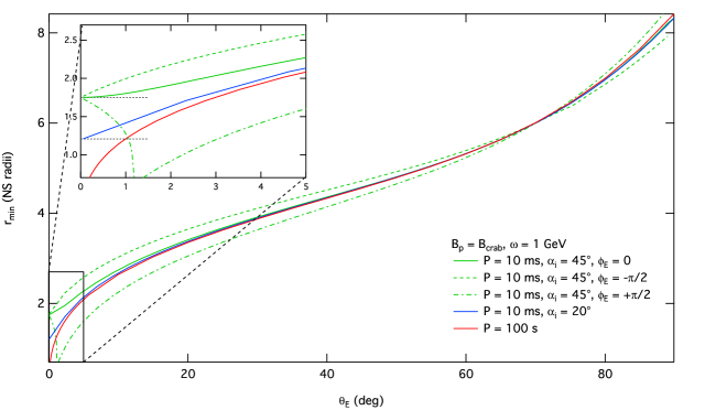
Figure 11.— Minimum altitudes of emission from the magnetic pole to the magnetic equator, for different sets of pulsar parameters. The Crab field value was adopted. As in Fig. 10, the dot-dash curves represent photons emitted on the leading side of the magnetic pole (evincing non-monotonic behavior of $\,r_{\rm min}\,$ with $\,\theta_{\hbox{\sixrm E}}\,$ – see inset), and dashed curves represent photons emitted on the trailing side of the pole. The gray dotted lines in the inset represent the zero-colatitude analytic approximation in Eq. (70).

Fig. 11 shows the effect of rotational aberration on the minimum altitudes of emission of 1 GeV photons; similar behavior is exhibited for other test photon energies. The surface polar magnetic field is again chosen to be the Crab value. Such altitude bounds are plotted as functions of emission colatitude, and except for very close to the pole, are generally well below the altitude of the last open field line. The red curve is a pulsar with a period of 100 sec, where aberration effects are minimal. The blue and green curves represent photons emitted from an azimuthal angle of zero for pulsars with periods of 10 seconds and inclination angles of 20 and 45 degrees, respectively. Green dotted and dashed lines represent photons emitted from the leading side of the magnetic pole (with the direction of rotation) and the trailing side (against the direction of rotation). Gray dashed lines again represent the $\,\theta_{\hbox{\sixrm E}}=0\,$ limit calculated from Eq. (70), so that $\,r_{\rm min}/R_{\hbox{\sixrm NS}}\,$ would represent the $\,h\,$ value that precisely generates an escape energy of 1 GeV in Eq. (71). It should be noted that like Lee et al. (2010), these calculations do not take pair threshold effects into account; by inspection of Fig. 10, it is apparent that corrections produced by accurately treating the threshold are small overall for the Crab field. In addition, we have not considered the full Kerr metric calculation, which would correctly account for aberration and general relativity together. Given the small nature of aberration influences overall on $\,\gamma\to e^{+}e^{-}\,$ pair opacity considerations at low to moderate altitudes, addressing this complication is not strongly motivated.

Very near the magnetic pole, i.e. $\,\theta_{\hbox{\sixrm E}}\lesssim 0.3^{\circ}\,$, aberration modifications increase the minimum emission altitude substantially for all azimuthal angles. The finite value of $\,\beta_{p}\,$ causes a photon emitted parallel to the magnetic field in the star frame to reach the minimum angle for pair production much earlier than for the non-rotating case, thus sharply decreasing the photon mean free path at low altitudes. Consequently, the minimum altitude is generally higher than for the $\,\beta_{p}=0\,$ situation. Moving away from the pole, the asymmetry between the leading and trailing sides of the magnetic pole becomes apparent. The trailing side sees a small increase in minimum altitudes, as field line crossing becomes easier. The leading side sees a sharp valley in minimum altitude (see inset), paralleling the peak in escape energies in Fig. 10. Note that $\,r_{\rm min}\,$ values below the surface are indeed possible, and indicate transparency to $\,\gamma\to e^{+}e^{-}\,$ for emission near the pole. For colatitudes larger than around $\,5^{\circ}\,$, the small absolute changes to $\,\sin\theta_{\hbox{\sevenrm kB}}\,$ are swamped by the rapidly decreasing magnetic field. Finally, near the magnetic equator when altitudes are highest and thus aberration effects are at their strongest ($\,\beta_{\hbox{\sixrm E}}\gg\beta_{p}\,$), the asymmetry between the leading and trailing sides reappears, while $\,\phi_{\hbox{\sixrm E}}=0\,$ curves are barely altered from the $\,\beta_{p}\approx 0\,$ (i.e. 100 ms) case. In summation, aberration corrections alter the minimum altitudes relative to the non-rotating calculations most significantly at small colatitudes.

Figure 3 of Lee et al. (2010) presents calculations of the minimum altitude of emission as a function of emission colatitude for different photon energies and pulsar inclination angles. Our results differ from theirs in a number of important respects. For the smallest pulsar inclination angles $\,\alpha_{i}\,$, the minimum altitudes of emission should approach the limit for a non-rotating neutron star, regardless of the other properties of the pulsar; our computations clearly display this characteristic. Fig. 11 indicates that the minimum altitude of emission is a monotonically increasing function of emission colatitude all the way up to equatorial emission at $\,\theta_{\hbox{\sixrm E}}=90^{\circ}\,$. It is not clear why the minimum altitudes obtained by Lee et al. (2010) decrease sharply at large colatitudes and especially why this effect is not noticeably weaker for $\,\alpha_{i}=15^{\circ}\,$ than for $\,\alpha_{i}=86^{\circ}\,$. In contrast, our computations realize intuitively sensible behavior: at equatorial colatitudes, photons more readily cross field lines after emission, and so one expects the minimum altitude for pair transparency to increase, sampling lower fields at and above the emission locale.

6. SOURCE CONNECTIONS: GAMMA-RAY PULSARS AND MAGNETARS

In this Section, we explore the implications of the pair transparency considerations for both gamma-ray pulsars and magnetars. The Fermi pulsar catalogues (Abdo et al., 2010a, 2013) provide us with a wealth of data for constraining the source regions for high energy emission from $\,\sim 140\,$ pulsars. The phase lag of the gamma-ray emission with respect to the radio emission can be used to estimate the altitude of the gamma-ray emitting region (Seyffert et al.  2012). Using relativistic descriptions of polarization position angle evolution, it can be determined (Blaskiewicz, Cordes, & Wasserman  1991) that the radio emission originates at typically $\,10-30R_{\hbox{\sixrm NS}}\,$ above the magnetic pole. Since the gamma-ray emission in outer magnetospheric models is usually significantly offset from the magnetic polar axis, the phase lag $\delta$ is a key parameter for narrowing the solution space in combined radio and gamma-ray light curve modeling. The gamma-ray peak separation, available for pulsars with 2 or more gamma-ray peaks, can also be compared to light curve modeling results to estimate the altitude of the emitting region (Watters et al.  2009; Venter, Johnson & Harding  2012). These generally conclude that the active zone is at altitudes $\,0.03R_{\hbox{\sixrm LC}}-R_{\hbox{\sixrm LC}}\,$, with determinations sensitively depending on the obliquity of the rotator and the observer’s viewing perspective.

Such geometric limits on the emission altitudes generally place the source of $\,\sim\,$GeV gamma rays in the outer magnetosphere (Pierbattista et al., 2010; Watters & Romani, 2011; Pierbattista et al., 2014). The complementary emission radii lower bounds calculated in this paper from magnetic pair creation are mostly at much smaller altitudes than this, yet provide interesting constraints in some cases. In particular, in the absence of aberration they do not depend on the magnetic inclination of the pulsar and the observer viewing angle. Moreover, the pair transparency bounds can be used even if the pulsar is radio quiet (33 LAT pulsars as of October 2013) or has only a single gamma-ray peak (31 LAT pulsars; Abdo et al.  2013).

In acceleration gap models of gamma-ray emission from pulsars, the gaps are generally assumed to be located in a narrow band along the last open magnetic field line (e.g., Romani, 1996; Muslimov & Harding, 2004; Hirotani, 2007). This follows the precedent established in earlier polar cap models (Daugherty & Harding  1982) of gamma-ray pulsars. If we assume that emission takes place on and parallel to the last open field line, we can then calculate an approximate minimum radius of emission using the procedure in Section 3.2 with the general relativistic corrections of Section 4. We therefore use pair transparency to provide a physical lower bound to $\,r_{\rm min}\,$. These minimum radii depend on assumptions about the neutron star mass and radius to only a small extent. For example, doubling the assumed mass of the neutron star increases the minimum radii by approximately 5% at most near the surface, with the change being due to general relativistic influences. In addition, they are independent of the inclination of the neutron star when aberration is unimportant (mostly the case). Using the Erber approximation result in Eq. (20), it is simply determined that for fixed $\,\varepsilon_{\rm esc}\,$, one should expect a correlation of $\,r_{\rm min}^{5/2}\propto\varepsilon_{\rm esc}B_{p}\theta_{f}\propto B_{p}/\sqrt{P}\,$, using the approximate polar cap footpoint colatitude dependence $\,\theta_{f}\equiv\theta_{p}\approx\sqrt{2\pi R_{\hbox{\sixrm NS}}/(Pc)}\propto P^{-1/2}\,$. If one neglects the second logarithmic ($\,B_{p}\,$-dependent) term inside the parentheses in Eq. (20), this flat space-time correlation is approximately

$$\hbox{${{\displaystyle r_{\rm min}\vphantom{(}}\over{\displaystyle R_{\hbox{\sixrm NS}}\vphantom{(}}}$}\;\approx\;0.037\varepsilon_{\rm esc}^{2/5}\,10^{2\sigma_{\rm IG}/5}\quad,\quad\sigma_{\rm IG}\;=\;\log_{10}\left(\hbox{${{\displaystyle B_{12}\vphantom{(}}\over{\displaystyle\sqrt{P}\vphantom{(}}}$}\right)\quad,$$ (72)

where the unscaled polar field is $\,B_{p}=B_{12}10^{12}\,$Gauss, and we set $\,R_{\hbox{\sixrm NS}}=10^{6}\,$cm. For the purposes of this discussion, here we adopt the relation $\,B_{p}\approx 6.4\times 10^{19}\sqrt{P\,{\dot{P}}}\,$ for the unscaled field, which corresponds to the vacuum magnetic dipole moment $\,\mu=B_{p}R_{\hbox{\sixrm NS}}^{3}/2\,$ (Shapiro & Teukolsky, 1983; Usov & Melrose, 1995), and is twice the conventional choice of Manchester & Taylor (1977) that is applicable to the equatorial surface field. Note that non-dipolar contributions and plasma loading of the magnetosphere modify such inferences of pulsar surface fields from $\,P\,$ and $\,\dot{P}\,$.

Fig. 12 shows the minimum radii of emission for the pulsars listed in the second Fermi catalog, plotted against $\,\sigma_{\rm IG}\,$, a proxy for the logarithm of $\,B_{p}/\sqrt{P}\,$. These minimum radii are calculated using a test photon energy that is twice the cutoff energy $E_{c}$ published in the catalog paper (Abdo et al.  2013). The choice of $\,2E_{c}\,$ does not exactly represent the highest energy photons detected from the source, but is slightly above the energy where the $\,\nu F_{\nu}\,$ is at a maximum, modulo a factor that depends on the power-law spectral index below the cutoff. The cutoff energies from the fits range from 0.4 to 5.9 GeV for the sources where spectral fitting produces significant determinations of $\,E_{c}\,$; the Crab pulsar is an exceptional case that will be isolated below. The handful of pulsars with poor spectral fits in Table 9 of Abdo et al.  (2013) are not included in this analysis.

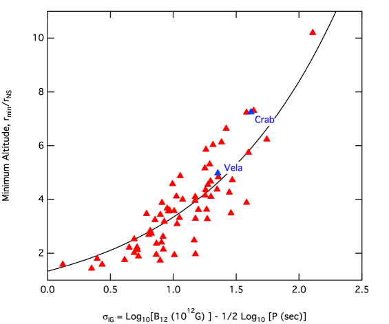
Figure 12.— Minimum emission radii for a selection (see text) of young pulsars among the 117 pulsars in the second Fermi pulsar catalog (Abdo et al., 2013). The minimum radius in neutron star radii is plotted against a scaling of the logarithm of $\,B_{12}/\sqrt{P}\,$. This couples directly to the dependence suggested in Eq. (72) for flat space-time, an indication of which is provided by the black curve, which represents $\,r_{\rm min}/R_{\hbox{\sixrm NS}}=4/3\times 10^{2\sigma_{\rm IG}/5}\,$. These minimum radii are found by solving $\,\tau(r_{\hbox{\sixrm E}},\varepsilon_{c})=1\,$ for $\,r_{\hbox{\sixrm E}}\,$, using twice the exponential cutoff energies $\,E_{c}\,$ measured by Fermi-LAT (Abdo et al.  2013), and assuming that emission takes place on the last open field line. If the same calculation is done for the VERITAS detection of the Crab pulsar at 120 GeV, we get a minimum radius of $\,20R_{\hbox{\sixrm NS}}\,$, while the MAGIC claim of pulsed emission up to $\,350-400\,$GeV would raise the bound to $\,r_{\rm min}\sim 31R_{\hbox{\sixrm NS}}\,$; both far exceed the minimum radius of $\,7.25R_{\hbox{\sixrm NS}}\,$ obtained from the Fermi cutoff energy.

Pulsars with magnetic fields too low for magnetic pair creation to play a significant role in propagation of GeV-band photons in their magnetospheres, including nearly all millisecond pulsars, are not constrained at all by this technique; their pair attenuation “minimum radii” are not only inside the neutron star, but inside the Schwarzschild radius, and therefore not meaningful. As an example, PSR B1821-24 in the globular cluster M28, with its period $\,P=3.05\,$ms and period derivative $\,{\dot{P}}=1.62\times 10^{-18}\,$sec sec^-1, possesses the highest known spin-down luminosity of any MSP (Johnson, et al., 2013). Its surface polar field is $\,B_{p}\approx 4.5\times 10^{9}\,$Gauss, i.e. approximately $\,10^{-4}B_{\rm cr}\,$. One can infer from Fig. 3 that its polar cap angle of $\,\approx 15^{\circ}\,$ would then yield an escape energy of around 30 GeV, a factor of 100 higher than for the $\,B_{p}=0.01\,$ case illustrated therein. This $\,\varepsilon_{\rm esc}\,$ is above the turnover energy $\,E_{c}\sim 6\,$GeV determined in the pulsed Fermi-LAT data in Johnson, et al. (2013), so that pair transparency for all photons detected by the LAT can be presumed at altitudes above the surface.

The $\,r_{\rm min}\,$ values in Fig. 12 display a general increase with $\,\sigma_{\rm IG}\,$, but considerable scatter. The relation in Eq. (72) is schematically represented in the Figure via the black curve $\,r_{\rm min}/R_{\hbox{\sixrm NS}}=4/3\times 10^{2\sigma_{\rm IG}/5}\,$, corresponding to a value of $\,\varepsilon_{\rm esc}\approx 4\times 10^{3}\,$ (i.e., 2.0 GeV) in Eq. (72). This defines the general character of the minimum altitude calculations, so that the scatter expresses the distribution of $\,E_{c}\,$ values in the Fermi pulsar spectral database. The point in the top right corner, with an $\,r_{\rm min}\,$ value over $\,10R_{\hbox{\sixrm NS}}\,$, is for PSR J1119-6127, a high-field pulsar with a surface polar field well above the quantum critical value. For the Crab and Vela pulsars, the minimum radii calculated using the Fermi-LAT cutoff energies are indicated on the plot. If one performs the same calculation for the VERITAS detection of pulsed emission from the Crab pulsar at 120 GeV (Aliu et al.  2011), the minimum emission radius for those 120 GeV photons is approximately $\,20R_{\hbox{\sixrm NS}}\,$. Even more interestingly, the MAGIC experiment has displayed evidence of pulsed emission from the Crab up to 350–400 GeV (see Fig. 4 of Aleksić et al., 2012), for which the $\,r_{\rm min}\,$ determination increases to around $\,31R_{\hbox{\sixrm NS}}\,$, or approximately $\,0.2R_{\hbox{\sixrm LC}}\,$. This is a profound constraint that impacts the discussion of slot gap versus outer gap models of the Crab, and is completely independent of altitude inferences from pulse profile geometric analyses. Observe that if the lower spin-down field estimate of Manchester & Taylor (1977) is adopted, this bound drops only to $\,r_{\rm min}\approx 23R_{\hbox{\sixrm NS}}\approx 0.15R_{\hbox{\sixrm LC}}\,$, still offering an important constraint. Note also that at these altitudes, one might expect rotational aberration to be influential, perhaps more so in the trailing edge of emission. By inspection of the altitude bound in Fig. 11 for lower energy (GeV) photons, we anticipate that aberration will provide at most a modest modification to this $\,r_{\rm min}\sim 0.2R_{\hbox{\sixrm LC}}\,$ determination.

To provide a striking contrast to this case, the same analysis can be performed for the softest Fermi-LAT gamma-ray pulsar, PSR J1513-5908 (B1509-58), whose signal extends only out to around 230 MeV. This high-field pulsar has a period of $\,151\,$ms, is fairly faint in the LAT band (Abdo et al., 2010d) and is detected by AGILE (Pilia et al., 2010), also out to around 200-300 MeV. It was not detected by EGRET on the Compton Gamma-Ray Observatory, but was seen by COMPTEL at energies below 30 MeV (Kuiper et al., 1999). Using 230 MeV to set $\,\varepsilon_{\rm esc}\,$, we infer a minimum emission radius of approximately $\,2.3R_{\hbox{\sixrm NS}}\,$. While this is not constraining for slot gap and outer gap models, it is of significant interest that it is somewhat above the surface. The broad pulse profile (Abdo et al., 2010d) implies that a more substantial range of emission altitudes can be accommodated than is typical for gamma-ray pulsars. Moreover, the fact that one of the gamma-ray peaks very slightly leads the radio pulse peak (Abdo et al., 2010d) may be an indicator of a polar cap type component to the pulsar’s signal. Early interpretation of the EGRET upper limits argued for the action of photon splitting in the strong fields near the surface of PSR J1513-5908 (Harding, Baring & Gonthier, 1997), which has $\,B_{p}=3.1\times 10^{13}\,$Gauss. This suggestion was predicated on the contention that polar cap models could account for the emission in this pulsar, and required the gamma-ray attenuation by the splitting process to arise proximate to the polar cap. The pair transparency altitude bound computed here indicates that the magnetic field local to the emission of $\,\sim 230\,$MeV photons is less than $\,\sim 2.4\times 10^{12}\,$Gauss, a lower field domain that strongly inhibits photon splitting opacity (e.g., Baring & Harding, 2001) in a neutron star magnetosphere.

It should be noted that if the magnetic field includes higher-order multipole components, as in Arons & Scharlemann (1979), the minimum emission radii calculated using this technique will change. The addition of a toroidal component to the magnetic field will increase the magnetic field magnitude and decrease the field line radius of curvature in most of the inner magnetosphere, which will make it easier for photons to transit across field lines and thereby enhance the attenuation of photons by magnetic pair creation. This must then be compensated by moving the emission regions to higher altitudes where the field is lower. For this case, therefore, our $\,r_{\rm min}\,$ estimates serve as conservative lower limits. An off-center dipole magnetic field (e.g., Harding & Muslimov, 2011) will introduce an asymmetry in field magnitude and radius of curvature, which will bring $\,r_{\rm min}\,$ down on the “stretched” side and raise it up on the “compressed” side. This provides a modest range of minimum altitudes so that our computations serve as approximate guides. We anticipate that the modifications introduced by offset dipolar morphology are tantamount to selecting a field line of slightly different footpoint colatitude from that for the last open field line in a true dipole field; interpretation of the numerical results presented here can then be adjusted accordingly.

The second observational context considered here concerns magnetars, namely soft gamma repeaters (SGRs) and anomalous X-ray pulsars (AXPs). With their supercritical fields, these energetic cousins of pulsars possess steady pulsed emission that is very different from that of gamma-ray pulsars. They have prominent thermal X-ray emission below 10 keV, and virtually equally luminous hard X-ray emission (e.g., Kuiper, Hermsen & Mendez, 2004; Goetz, et al., 2006; den Hartog, Kuiper, Hermsen, et al., 2008; den Hartog, Kuiper & Hermsen, 2008) that is well-described by power-law tails. These flat tails cannot extend beyond energies of a few hundred keV due to constraining upper limits obtained by the COMPTEL instrument on the Compton Gamma-Ray Observatory. A prominent model for the tail emission is that it is due to inverse Compton scattering of surface thermal X-rays by relativistic electrons in the strong fields of the inner magnetosphere (Baring & Harding, 2007; Nobili, Turolla & Zane, 2008; Baring, Wadiasingh & Gonthier, 2011; Beloborodov, 2013). Such emission should then be subject to the magnetic pair attenuation that is the focus of this paper. Here we determine the energy ranges for which pair opacity should strongly attenuate the tail spectra. Magnetars also exhibit flaring episodes, ranging in luminosity up to the giant flares seen in three soft gamma repeaters. This emission also does not extend beyond about 1 MeV. A comprehensive observational and theoretical summary of magnetars can be found in Mereghetti (2008).

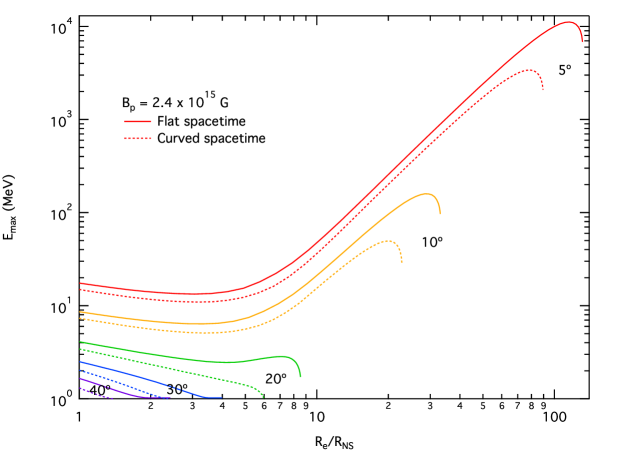
Figure 13.— Pair creation escape energies $\,\varepsilon_{\rm esc}\,$ for photons emitted along four different field lines of a magnetar with a surface polar magnetic field of $\,2.4\times 10^{15}\,$Gauss. These are plotted as functions of the radius of emission in neutron star radii. Curves are labeled with the “footpoint colatitude” of the field line, and the selected values ($\,\theta_{f}=5^{\circ},10^{\circ},20^{\circ},30^{\circ},40^{\circ}\,$) correspond to the closed field line region. Solid curves represent flat spacetime and dashed curves fully include general relativistic effects. For emission below 10 stellar radii, one would not expect photons to emerge from the magnetosphere above around 10 MeV.

For magnetar applications, the asymptotic approximations to the attenuation rate given in Eqs. (2) and (3) are not applicable at low altitudes, and the full form of the rate given in Daugherty & Harding (1983) must be used, i.e. that embodied in Eqs. (5) and (6). This is because for magnetic fields above $\,B_{\rm cr}\,$, the pair conversion optical depth is sensitive to the individual thresholds for each Landau level transition. We use here a hybrid protocol that calculates the attenuation rate for the lowest two Landau levels exactly, and at higher energies uses the BK07 asymptotic form. The magnetic pair creation escape energies for photons emitted along dipole magnetic field lines are plotted as a function of altitude of emission in Fig. 13. Each set of curves is labeled with the footpoint colatitude of the field line when it intersects the magnetar surface. Aberration influences are omitted in these calculations, although GR modifications are included for the curves indicated. The differences in $\,\varepsilon_{\rm esc}\,$ values between the general relativistic and flat spacetime results are manifested for all altitudes because for a fixed footpoint colatitude, GR distorts the field line at all altitudes, increasing the curvature so that it crosses the magnetic equator at a smaller radius. Accordingly, the escape energies are lowered slightly. If one were to plot results for the last open field line, the footpoint colatitudes would differ between flat spacetime and GR cases according to Eq. (47), but the $\,\varepsilon_{\rm esc}\,$ curves would merge at moderate to high altitudes.

The surface polar magnetic field used for this plot is $\,2.4\times 10^{15}\,$Gauss, half the estimated surface magnetic field strength for SGR 1806-20 and somewhat above the corresponding value for SGR 1900+14. At typical magnetar periods, the polar cap size (angle $\,\theta_{p}\,$) is less than 1 degree, so all of these curves represent emission taking place in the closed field line region. All photons with energies above these $\,\tau(\varepsilon_{\rm esc})=1\,$ curves will be absorbed via magnetic pair creation before they can escape to infinity. Since these curves are computed for cases where emission is presumed to be beamed along field lines, for non-zero initial $\,\theta_{\hbox{\sevenrm kB}}\,$ angles, the opacity will increase dramatically and reduce $\,\varepsilon_{\rm esc}\,$ so that these bounds will become more stringent.

The curves in Fig. 13 decline at first with increasing emission altitude, and then exhibit pronounced rises. The weak decline is associated with the regime of pair creation near threshold when the field at $\,r_{\hbox{\sixrm E}}\,$ is near-critical or supercritical, up to around $\,r_{\hbox{\sixrm E}}/R_{\hbox{\sixrm NS}}\sim 3-6\,$. In this portion of parameter space, $\,\varepsilon_{\rm esc}\,$ is relatively insensitive to the field strength, and drops slightly with rising $\,r_{\hbox{\sixrm E}}\,$ since increasing field line curvature allows photons to more readily propagate across field lines. The curves then transition into emission altitudes where the field is subcritical, and the familiar $\,\varepsilon_{\rm esc}\propto r_{\hbox{\sixrm E}}^{5/2}\,$ in Eq. (20) is approximately realized — this is clearly evident in the $\,5^{\circ}\,$ footpoint colatitude case. The turndowns at the extreme highest altitudes correspond to quasi-equatorial emission cases where the photons again readily transit across field lines that exhibit greater flaring. Smaller radii of field line curvature are also responsible for the trend of declining escape energy with increasing footpoint colatitude $\,\theta_{f}\,$, with an approximate dependence $\,\varepsilon_{\rm esc}\propto 1/\theta_{f}\,$ when $\,\theta_{f}\ll 1\,$. For somewhat lower surface polar field cases that are not shown, for near-surface emission the escape energy rises, but not dramatically, since pair creation still occurs near the $\,2m_{e}c^{2}\,$ threshold. This situation is applicable to the lower field magnetars such as AXP 4U 0142+61 and AXP 2259+586 which possess $\,B_{p}=2.7\times 10^{14}\,$Gauss and $\,B_{p}=1.2\times 10^{14}\,$Gauss, respectively. In particular, the $\,\varepsilon_{\rm esc}\propto r_{\hbox{\sixrm E}}^{5/2}\,$ domain for $\,\theta_{f}=5^{\circ},10^{\circ}\,$ then penetrates to lower emission altitudes in such cases, and $\,\varepsilon_{\rm esc}\,$ rises at higher $\,r_{\hbox{\sixrm E}}\,$, as the magnetar environment starts to transition towards the sub-critical $\,B_{p}\,$ regime that is treated in Fig. 7.

This opacity phase space plot clearly indicates that magnetars should not be visible to the Fermi-LAT telescope if their activation takes place in the inner magnetosphere, which is the preferred paradigm for twisted magnetosphere models (e.g., Beloborodov, 2009; Parfrey, Beloborodov & Hui, 2013) of magnetars. We can see, for example, that 100 MeV photons cannot escape at all from the region bounded by the closed field line that crosses the neutron star surface at a colatitude of $\,\theta_{f}=10^{\circ}\,$, and can only escape from the region bounded by the field line with a footpoint colatitude of $\,5^{\circ}\,$ if they originate more than 10 neutron star radii from the center of the star. This may explain the non-detection of 13 magnetars at Fermi-LAT energies (Abdo et al. 2010c; see also Şaşmaz Muş & Göğüş 2010) — any emission above 100 MeV must emanate from high altitude zones in the outer magnetosphere. This would have to be the case if the claim of a $\,5\sigma\,$ detection of pulsed emission above 200 MeV in a 4 year collection of Fermi-LAT public archive data for AXP 1E 2259+586 (Wu et al., 2013) is confirmed. Such evidence of pulsation in this source is not found in the analysis of Abdo et al. (2010c), and no public confirmation of the Wu et al. (2013) claim has been offered by the Fermi-LAT Collaboration to date. If emission from select magnetars at energies above 100 MeV is eventually verified, the pair attenuation studies presented here have important implications for the paradigms surrounding magnetar quiescent emission. If it is not confirmed, then pair opacity provides a natural explanation why magnetars are not seen in hard gamma-rays.

7. CONCLUSIONS

In this paper, single-photon (magnetic) pair creation transparency conditions for neutron star magnetospheres have been calculated, beginning with the simplest case of a non-rotating star in the absence of general relativistic effects, and progressing to sequentially consider curved spacetime and then the influences of rotational aberration. Optical depths are calculated for arbitrary photon emission points in neutron star magnetospheres in the special case where photons are initially parallel to the magnetic field. Such initial propagation conditions are expected in pulsars because electrons that emit curvature radiation gamma rays have such high Lorentz factors that all the photons will be subject to very strong relativistic beaming along B. A similar situation exists for magnetars, if their hard X-ray signals are generated by inverse Compton scattering using extremely relativistic electrons. The optical depth determinations enable the presentation of attenuation lengths, minimum altitudes of emission for a given energy, and escape energies for a given emission altitude, at various stages of the paper. In developing these results, we have presented a set of analytic and semi-analytic forms that greatly simplify the computation of magnetic pair creation opacities. These approximations can be applied to any emission altitude and most colatitudes, and were discussed in the contexts of gamma-ray pulsars and magnetars.

The principal findings of our analysis are as follows. Flat spacetime computations reproduce extant results in the literature nicely, and indicate that pair attenuation escape energies anti-correlate with the colatitude of emission and the surface polar field strength, as expected due to the mathematical character of the pair attenuation coefficient. The introduction of general relativistic modifications modestly reduces both attenuation lengths and escape energies for pair creation at low altitudes near the stellar surface, but provides almost negligible alteration from flat spacetime results above $\,\sim 5\,$ stellar radii. For the inner magnetospheric considerations germane to $\,\gamma\to e^{+}e^{-}\,$ opacity, rotational corrections to the static pair attenuation analyses are generally found to be quite limited, except for a small domain where photons are emitted approximately directly above the magnetic pole. In such cases, rotational aberration forces photons to propagate across field lines almost immediately after emission, as viewed by the distant, static observer. For emission colatitudes below around 3 degrees, depending on the directional phase of photon emission, aberration can either increase or decrease the instantaneous pair conversion rates relative to those for the non-rotating case, and accordingly the escape energy can either rise or decline.

For young pulsars, the paper generates estimates of the minimum altitude $\,r_{\rm min}\,$ that permits pair transparency out to the maximum gamma-ray energies detected by Fermi-LAT. These $\,r_{\rm min}\,$ values are one of the few constraints available on the emission location in gamma-ray pulsars with a single peak, and they have the advantage of being a physics-based constraint that is not solely dependent on the geometry of the emitting region. The minimum emission altitudes that we calculate from magnetic pair creation are normally far below those obtained from pulse profile fitting with slot gap or outer gap models, which are typically $\,r_{\rm min}>0.05R_{\hbox{\sixrm LC}}\,$ for two-peaked pulsars. They become much more useful constraints on curvature-radiation-based models for the significant number of single-peaked young pulsars, for which pulse profile modeling is not effective in the absence of a pulsed radio counterpart. Interestingly, for the Crab pulsar, the altitude bound rises to around $\,r_{\rm min}\sim 20R_{\hbox{\sixrm NS}}\,$ due to its energetic emission confirmed by both VERITAS and MAGIC out to 120 GeV; this bound is raised further to $\,r_{\rm min}\sim 31R_{\hbox{\sixrm NS}}\,$ when using the report of pulsed emission in MAGIC data out to 350–400 GeV. This most extreme bound is around 20% of the Crab’s light cylinder radius; it was obtained when omitting rotational aberration effects, which will modify the limit somewhat, but not drastically. Our results are clearly not applicable to millisecond pulsars, where the surface magnetic fields are too low for magnetic pair creation opacity to be significant. The pair creation calculations presented are germane to magnetars, and they indicate that soft gamma repeaters and anomalous X-ray pulsars should not be detectable above 100 MeV by Fermi-LAT unless their emission regions are generally at altitudes of around 10 stellar radii or higher.

Appendix A Appendix A: Approximating the Photon Trajectory Curvature Integral

The photon trajectory in curved spacetime is defined by colatitude $\,\theta\,$ expressed as an integral over the propagation altitude parameter $\,\Psi=r_{s}/r\,$, where $\,r_{s}\,$ is the neutron star’s Schwarzschild radius. The angle in Eq. (11) of GH94 is the difference between the angle (in the local inertial frame) of the photon momentum vector to the radial vector at the point of emission, and the angle of the photon trajectory to the local radial vector at a point defined by $\,\Psi\,$; it relates to $\,\theta\,$ as follows:

$$\theta(\Psi)\;\equiv\;\theta_{\hbox{\sixrm E}}+\Delta\theta\;=\;\theta_{\hbox{\sixrm E}}+\int_{\Psi}^{\Psi_{\hbox{\sixrm E}}}\frac{d\Psi_{r}}{\sqrt{\Psi_{b}^{2}-\Psi_{r}^{2}(1-\Psi_{r})}}\quad.$$ (A1)

Since $\,\Psi\leq\Psi_{\hbox{\sixrm E}}\,$ in this construction, as the photon propagates out from the star, then the change in colatitude $\,\Delta\theta\,$ is necessarily positive as the altitude $\,r\,$ increases. Also, $\,\Psi_{b}=r_{s}/b\,$ expresses the general relativistic impact parameter $\,b\,$ for the unbound photon path.

Computation of the trajectory using numerical integration is expensive in terms of time, particular for repeated applications in Monte Carlo simulations of magnetospheric cascades, so it is expedient to derive an analytic approximation to the integral in Eq. (39). Using manipulations outlined in Chapter 17 of Abramowitz & Stegun (1965), this integral can be expressed in terms of elliptic functions. Such a step does not facilitate its evaluation, since the parameter $\,\Psi_{\hbox{\sixrm E}}/\Psi_{b}\,$ is not necessarily small, a condition that would render series expansion of elliptic functions more amenable. In our neutron star cases, $\,\Psi_{\hbox{\sixrm E}}\lesssim 0.4\,$ is generally realized, and this suggests a series expansion in this parameter. To effect such, we have designed an expansion algorithm (not unique) that is motivated by the flat spacetime limit $\,\Psi_{\hbox{\sixrm E}}\to 0\,$ of the integral. Define

$$\rho_{f}\;=\;\sqrt{\Psi_{b}^{2}-\Psi_{r}^{2}}\quad,\quad\rho_{c}\;=\;\sqrt{\Psi_{b}^{2}-\Psi_{r}^{2}(1-\Psi_{r})}$$ (A2)

as flat and curved spacetime forms, respectively, of the denominator of the integrand of the trajectory integral. A Taylor series expansion for $\,\rho_{c}/\rho_{f}=\sqrt{1+\Psi_{r}^{3}/\rho_{f}^{2}}\,$ can be developed in the generally small parameter $\,\Psi_{r}^{3}/\rho_{f}^{2}\,$. Note that this parameter is not much less than unity for near-surface, equatorial cases. This protocol results in a series expansion in $\,\Psi_{b}\,$ for the integral:

$$\Delta\theta\;=\;\int^{\Psi_{\hbox{\sixrm E}}}_{\Psi}\hbox{${{\displaystyle d\Psi_{r}\vphantom{(}}\over{\displaystyle\rho_{f}\vphantom{(}}}$}\left\{1-\hbox{${{\displaystyle\Psi_{r}^{3}\vphantom{(}}\over{\displaystyle 2\rho_{f}^{2}\vphantom{(}}}$}+\hbox{${{\displaystyle 3\Psi_{r}^{6}\vphantom{(}}\over{\displaystyle 8\rho_{f}^{4}\vphantom{(}}}$}-\hbox{${{\displaystyle 5\Psi_{r}^{9}\vphantom{(}}\over{\displaystyle 16\rho_{f}^{6}\vphantom{(}}}$}+\hbox{${{\displaystyle 35\Psi_{r}^{12}\vphantom{(}}\over{\displaystyle 128\rho_{f}^{8}\vphantom{(}}}$}\right\}+O\left(\Psi_{\hbox{\sixrm E}}^{5}\right)\quad.$$ (A3)

Now define the scaled parameters

$$\Upsilon\;=\;\hbox{${{\displaystyle\Psi\vphantom{(}}\over{\displaystyle\Psi_{b}\vphantom{(}}}$}\quad,\quad\Upsilon_{\hbox{\sixrm E}}\;=\;\hbox{${{\displaystyle\Psi_{\hbox{\sixrm E}}\vphantom{(}}\over{\displaystyle\Psi_{b}\vphantom{(}}}$}\quad.$$ (A4)

The integrals in Eq. (A3) are all analytically tractable, and yield a useful analytic approximation for the photon trajectory:

$$\Delta\theta\;\approx\;\Delta\theta_{\hbox{\sevenrm app}}\;\equiv\;\biggl{[}\arcsin\upsilon-\Psi_{b}\,f_{1}(\upsilon)+\Psi_{b}^{2}\,f_{2}(\upsilon)-\Psi_{b}^{3}\,f_{3}(\upsilon)\biggr{]}^{\Upsilon_{\rm E}}_{\Upsilon}\quad,$$ (A5)

when retaining only the first four terms in the integrand of Eq. (A3). Here

$$f_{1}(\upsilon) = \hbox{${{\displaystyle 2-\upsilon^{2}\vphantom{(}}\over{\displaystyle 2\sqrt{1-\upsilon^{2}}\vphantom{(}}}$}-1$$

$$f_{2}(\upsilon) = \hbox{${{\displaystyle 15\vphantom{(}}\over{\displaystyle 16\vphantom{(}}}$}\,\arcsin\upsilon-\hbox{${{\displaystyle\upsilon\,(15-20\upsilon^{2}+3\upsilon^{4})\vphantom{(}}\over{\displaystyle 16\,(1-\upsilon^{2})^{3/2}\vphantom{(}}}$}$$ (A6)

$$f_{3}(\upsilon) = \hbox{${{\displaystyle 128-320\upsilon^{2}+240\upsilon^{4}-40\upsilon^{6}-5\upsilon^{8}\vphantom{(}}\over{\displaystyle 48(1-\upsilon^{2})^{5/2}\vphantom{(}}}$}-\hbox{${{\displaystyle 8\vphantom{(}}\over{\displaystyle 3\vphantom{(}}}$}\quad.$$

This provides an alternative to the Beloborodov (2002) approximation. As constructed, for small arguments $\,\upsilon\,$, the functions employed in the approximation scale as $\,f_{n}(\upsilon)\propto\upsilon^{1+3n}\,$. This regime is sampled for $\,\Psi_{b}\gg 1\,$, the low impact parameter cases appropriate for circumpolar colatitudes. Accordingly, the series implied by extension of Eq. (A5) to higher order terms is nicely convergent even when $\,\Psi_{b}\,$ is large.

For photon emission from the neutron star surface, with $\,\Psi_{\hbox{\sixrm E}}\approx 0.4\,$, this approximation for the transit in colatitude is accurate to better than 0.1% at all subsequent altitudes for emission colatitudes $\,\theta_{\hbox{\sixrm E}}\lesssim\pi/4\,$. Raising the altitude of emission, i.e. reducing $\,\Psi_{\hbox{\sixrm E}}\,$ below $\,0.1\,$ substantially improves this. This level of precision is entirely suitable for the pertinent pulsar parameter space, where footpoint colatitudes are usually inferior to $\,\theta_{f}\lesssim 30^{\circ}\,$. To illustrate this, in Fig. 14 we plot the fractional precision $\,|\Delta\theta_{\hbox{\sevenrm app}}/\Delta\theta-1|\,$ of the approximation in Eq. (A5) relative to the exact integral in Eq. (39) or Eq. (A1), as a function of $\,\Psi\,$ for different colatitudes $\,\theta_{\hbox{\sixrm E}}\,$ and altitudes $\,\Psi_{\hbox{\sixrm E}}\,$ representative of the locales sampled in the pair attenuation calculations. Given an emission altitude parameter $\,\Psi_{\hbox{\sixrm E}}\,$, the emission colatitude $\,\theta_{\hbox{\sixrm E}}\,$ can then be used to define the impact parameter $\,\Psi_{b}\,$ in Eq. (37). The precision clearly is degraded at high colatitudes, though is always better than 1% for the colatitudes illustrated. Yet, because the general relativistic curvature is diminished at higher emission altitudes, the range of colatitudes $\,\theta_{\hbox{\sixrm E}}\,$ yielding a given level of precision increases as $\,\Psi_{\hbox{\sixrm E}}\,$ declines. To retain 0.1% precision, it is best to restrict use of the approximation to field line footpoint colatitudes $\,\theta_{f}\lesssim 45^{\circ}\,$.

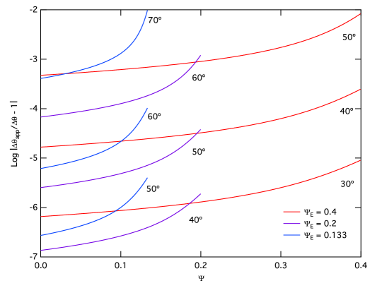
Figure 14.— The fractional precision $\,|\Delta\theta_{\hbox{\sevenrm app}}/\Delta\theta-1|\,$ of the approximation in Eq. (A5) to the full trajectory integral in Eq. (39) for photon propagation in curved spacetime. Three groups of curves, color-coded, are illustrated for altitude parameters $\,\Psi_{\hbox{\sixrm E}}=0.4,0.2,0.133\,$, as marked, corresponding to emission at the neutron star surface and at two and three stellar radii. The range of altitudes $\,0\leq\Psi\leq\Psi_{\hbox{\sixrm E}}\,$ spans from the emission locale all the way out to infinity. Within each group are three curves for emission colatitudes $\,\theta_{\hbox{\sixrm E}}\,$, as labelled, illustrating how the precision of the approximation improves nearer the magnetic axis.

Appendix B Appendix B: Approximating the Optical Depth for Zero-Colatitude Emission in a Rotating Magnetosphere

To facilitate semi-analytic checks on escape energies and minimum altitude numerics, we consider here the special case of aberration-corrected emission from directly above the magnetic pole ($\,\theta_{\hbox{\sixrm E}}=0\,$), for which the initial velocity and magnetic field vectors assume particularly simple forms. Using a combination of Eq. (57) and Eqs. (53) and (56) the direction of photon travel in the inertial observer frame simplifies to

$$\mathbf{\hat{k}_{O}}\;\approx\;\begin{bmatrix}\sin\alpha_{i}\\ -\beta_{\hbox{\sixrm E}}\\ \cos\alpha_{i}\end{bmatrix},$$ (B1)

where $\,\beta_{\hbox{\sixrm E}}=2\pi r_{\hbox{\sixrm E}}\sin\alpha_{i}/cP\equiv h\beta_{p}\,$ is the magnitude of the corotation velocity divided by $\,c\,$. In this result, we have used the fact that $\,\beta_{\hbox{\sixrm E}}\ll 1\,$ at the low to moderate altitudes of interest for this5B development. Remember that $\,\beta_{p}=R_{\hbox{\sixrm NS}}\sin\alpha_{i}/R_{\hbox{\sixrm LC}}\,$ is the corotation speed of the magnetic pole at the stellar surface. Then the angle between the photon trajectory and the radial direction in the observer frame, given by Eq. (68), reduces to the simple form

$$\delta_{E,0}\;\approx\;\arcsin\left(\hbox{${{\displaystyle 2\pi r_{\hbox{\sixrm E}}\sin\alpha_{i}\vphantom{(}}\over{\displaystyle Pc\vphantom{(}}}$}\right)\quad.$$ (B2)

Since $\,\beta_{\hbox{\sixrm E}}\ll 1\,$, this is approximately

$$\delta_{E,0}\;\approx\;\hbox{${{\displaystyle 2\pi r_{\hbox{\sixrm E}}\sin\alpha_{i}\vphantom{(}}\over{\displaystyle Pc\vphantom{(}}}$}\;\equiv\;h\beta_{p}\quad.$$ (B3)

As in Eq. (11) we define $\,\chi\,$ to be the radial distance of the photon from the center of the neutron star divided by the radius of emission. Applying the law of sines, we have

$$\chi\;=\;\hbox{${{\displaystyle\sin\delta_{E,0}\vphantom{(}}\over{\displaystyle\sin(\delta_{E,0}-\eta)\vphantom{(}}}$}\;\approx\;\hbox{${{\displaystyle 1\vphantom{(}}\over{\displaystyle 1-\eta/\delta_{E,0}\vphantom{(}}}$}\quad,$$ (B4)

since both $\,\delta_{E,0}\,$ and $\,\eta\,$ are small. Accordingly, escape to infinity corresponds to $\,\eta\to\delta_{E,0}\,$. Similarly, for $\,s\,$, the law of sines and small-angle approximations give

$$s\approx r_{\hbox{\sixrm E}}\left(\chi-1\right).$$ (B5)

These can be carried through the coordinate transformations to express the approximate coordinates for the photon path in the star frame in terms of $\,\eta\,$:

$$r_{\hbox{\sixrm S}}\;\approx\;\frac{r_{\hbox{\sixrm E}}}{1-\eta/\delta_{E,0}}\quad,\quad\theta_{\hbox{\sixrm S}}\;\approx\;\eta\quad,\quad\phi_{\hbox{\sixrm S}}\;\approx\;-\hbox{${{\displaystyle\pi\vphantom{(}}\over{\displaystyle 2\vphantom{(}}}$}\quad.$$ (B6)

Observe that $\,\phi_{\hbox{\sixrm S}}\approx-\pi/2\,$ is an angular restriction that follows from the rotation velocity $\,\vec{\beta_{\hbox{\sixrm E}}}=\mathbf{\Omega}\times\mathbf{r_{\hbox{\sixrm E}}}\,$ at the point of emission being approximately orthogonal to the plane defined by $\,\vec{\mu}\,$ and $\,\mathbf{\Omega}\,$, since $\,\mathbf{r_{\hbox{\sixrm E}}}\,$ is nearly parallel to $\,\vec{\mu}\,$. With these approximations one can obtain a relatively compact form for the magnetic field and photon trajectory vector in the star frame. For the field we have

$$\mathbf{B_{S}}\;\approx\;\hbox{${{\displaystyle 3B_{p}R_{\hbox{\sixrm NS}}^{3}\vphantom{(}}\over{\displaystyle 2r_{\hbox{\sixrm E}}^{3}\vphantom{(}}}$}\left(1-\hbox{${{\displaystyle\eta\vphantom{(}}\over{\displaystyle\delta_{E,0}\vphantom{(}}}$}\right)^{3}T_{\Omega}(t_{\hbox{\sixrm O}})\cdot\begin{bmatrix}\hbox{${{\displaystyle 2\vphantom{(}}\over{\displaystyle 3\vphantom{(}}}$}\,\sin\alpha_{i}\\ -\eta\\ \hbox{${{\displaystyle 2\vphantom{(}}\over{\displaystyle 3\vphantom{(}}}$}\,\cos\alpha_{i}\end{bmatrix}\quad,$$ (B7)

which, using $\,\Omega t_{\hbox{\sixrm O}}\approx s/R_{\hbox{\sixrm LC}}\approx\delta_{E,0}\eta/[(\delta_{E,0}-\eta)\,\sin\alpha_{i}]\ll 1\,$ and Eqs. (B2), (B3) and (B4), is easily shown to be approximately equivalent to

$$\mathbf{B_{S}}\;\approx\;\hbox{${{\displaystyle B_{p}\vphantom{(}}\over{\displaystyle h^{3}\vphantom{(}}}$}\left(1-\hbox{${{\displaystyle\eta\vphantom{(}}\over{\displaystyle\delta_{E,0}\vphantom{(}}}$}\right)^{3}\begin{bmatrix}\sin\alpha_{i}\\ -\hbox{${{\displaystyle 3\vphantom{(}}\over{\displaystyle 2\vphantom{(}}}$}\,\eta+\hbox{${{\displaystyle\delta_{E,0}\eta\vphantom{(}}\over{\displaystyle\delta_{E,0}-\eta\vphantom{(}}}$}\\ \cos\alpha_{i}\end{bmatrix}\quad,$$ (B8)

The photon momentum vector is

$$\mathbf{k_{S}}\;\approx\;\omega\begin{bmatrix}\sin\alpha_{i}\\ \hbox{${{\displaystyle\delta_{E,0}\eta\vphantom{(}}\over{\displaystyle\delta_{E,0}-\eta\vphantom{(}}}$}\\ \cos\alpha_{i}\end{bmatrix}\quad,$$ (B9)

where the $\,y\,$ component is far inferior to the other two. The magnitude of the cross product $|\mathbf{k_{S}}\times\mathbf{B_{S}}|$ then has a leading order term given by

$$\Bigl{|}\mathbf{k_{S}}\times\mathbf{B_{S}}\Bigr{|}\;\approx\;\hbox{${{\displaystyle 3\omega B_{p}\vphantom{(}}\over{\displaystyle 2h^{3}\vphantom{(}}}$}\,\hbox{${{\displaystyle\eta\left(\delta_{E,0}-\eta\right)^{3}\vphantom{(}}\over{\displaystyle\delta_{E,0}^{3}\vphantom{(}}}$}\quad.$$ (B10)

Note that in this identity, and also in Eq. (B9), we can replace $\,\omega\,$ by the observer frame photon energy $\,\varepsilon\,$ since the Doppler shift in Eq. (58) simplifies for this $\,\beta_{\hbox{\sixrm E}}\ll 1\,$ case.

With all the quantities in Eq. (51) defined in terms of the small variable $\,\eta\,$, the integral can then be approximated as in Section 3.1 using the method of steepest descents. The peak of the integrand occurs at

$$\eta_{pk}\;=\;\hbox{${{\displaystyle\delta_{E,0}\vphantom{(}}\over{\displaystyle 4\vphantom{(}}}$}\quad,$$ (B11)

as we found for the non-rotating, flat spacetime case. In practice, the attenuation rate drops to almost zero well below $\,\eta_{max}\approx\delta_{E,0}\,$, due to the rapid decline in the field strength at high altitudes, and therefore we set $\,\eta_{\max}\to\infty\,$ in the steepest descents protocol. This then yields

$$\tau\;=\;\int_{0}^{\eta_{max}}\overline{R}\frac{ds}{d\eta}d\eta\;\approx\;\hbox{${{\displaystyle 3^{6}\sqrt{3}\vphantom{(}}\over{\displaystyle 2^{18}\vphantom{(}}}$}\,\hbox{${{\displaystyle\alpha_{f}\vphantom{(}}\over{\displaystyle\lambda\hbox to0.0pt{\hss--}\vphantom{(}}}$}\,\hbox{${{\displaystyle B_{p}R_{\hbox{\sixrm NS}}^{3}\vphantom{(}}\over{\displaystyle r_{\hbox{\sixrm E}}^{2}\vphantom{(}}}$}\sqrt{\frac{8\pi^{4}B_{p}R_{\hbox{\sixrm NS}}^{3}\varepsilon\sin^{3}\alpha_{i}}{c^{3}P^{3}}}\;\exp\left\{-\frac{2^{11}cPr_{\hbox{\sixrm E}}^{2}}{3^{5}\varepsilon B_{p}\pi R^{3}\sin\alpha_{i}}\right\}\quad,$$ (B12)

which can be recast slightly as Eq. (70). This satisfyingly simple result emerging from the complexity of aberration considerations is only applicable in the limit of non-relativistic boosts at low altitudes between the star and observer frames: it can be reliably applied when $\,R_{\hbox{\sixrm LC}}/R_{\hbox{\sixrm NS}}\gtrsim 30\,$, which includes all Fermi young gamma-ray pulsars. To determine the threshold for pair transparency, we set this integral equal to unity, and solve for one of the variables in terms of the others. From this analysis, it is clear that when $\,\theta_{\hbox{\sixrm E}}\rightarrow 0\,$, the minimum altitude for pair transparency for a given photon energy will attain a non-zero value and the escape energy for a photon emitted from a given altitude will remain finite.

References

- Abdo et al. (2009a) Abdo, A. A., Ackermann, M., Ajello, M., et al. 2009a, Science, 325, 840.
- Abdo et al. (2009b) Abdo, A. A., Ackermann, M., Atwood, W. B., et al. 2009b, ApJ, 696, 1084.
- Abdo et al. (2010a) Abdo, A. A., Ackermann, M., Ajello, M., et al. 2010a, ApJS, 187, 460.
- Abdo et al. (2010b) Abdo, A. A., Ackermann, M., Ajello, M., et al. 2010b, ApJ, 713, 154.
- Abdo et al. (2010c) Abdo, A. A., Ackermann, M., Ajello, M., et al. 2010c, ApJ, 725, L73.
- Abdo et al. (2010d) Abdo, A. A., Ackermann, M., Ajello, M., et al. 2010d, ApJ, 714, 927.
- Abdo et al. (2013) Abdo, A. A., Ackermann, M., Allafort, A., et al. 2013, ApJS, 208, 17.
- Aleksić et al. (2012) Aleksić, J., Alvarez, E. A., Antonelli, L. A., et al. 2012, A&A, 540, A69.
- Aliu et al. (2011) Aliu, E., Arlen, T., Aune, T., et al. 2011, Science, 334, 69.
- Arons & Scharlemann (1979) Arons, J. & Scharlemann, E. T. 1979, ApJ, 231, 854.
- Baier & Katkov (2007) Baier, V. N. & Katkov, V. M. 2007, Phys. Rev. D, 75, 073009.
- Baring (1988) Baring, M. G. 1988, MNRAS, 235, 79.
- Baring (1991) Baring, M. G. 1991 A&A, 249, 581.
- Baring (2004) Baring, M. G. 2004, Adv. Space Res., 33, 552.
- Baring & Harding (2001) Baring, M. G. & Harding, A. K. 2001, ApJ, 547, 929.
- Baring & Harding (2007) Baring, M. G. & Harding, A. K. 2007, Ap&SS, 308, 109.
- Baring, Wadiasingh & Gonthier (2011) Baring, M. G., Wadiasingh, Z. & Gonthier, P. L. 2011, ApJ, 733, 61.
- Beloborodov (2009) Beloborodov, A. M. 2009, ApJ, 703, 1044.
- Beloborodov (2013) Beloborodov, A. M. 2013, ApJ, 762, 13.
- Blaskiewicz, Cordes, & Wasserman (1991) Blaskiewicz, M., Cordes, J. M., & Wasserman, I. 1991, ApJ, 370, 643.
- Bucciantini, Arons & Amato (2011) Bucciantini, N., Arons, J. & Amato, E. 2011, MNRAS, 410, 381.
- Chang, Chen, & Ho (1996) Chang, H.-K., Chen, K. & Ho., C. 1996, A&AS, 120, 81.
- Cheng, Ho, & Ruderman (1986) Cheng, K. S., Ho, C. & Ruderman, M. A. 1986, ApJ, 300, 500.
- Chiang & Romani (1994) Chiang, J. & Romani, R. W. 1994, ApJ 436, 754.
- Daugherty & Harding (1982) Daugherty, J. K. & Harding A. K., 1982, ApJ, 252, 337.