Three-dimensional nonparaxial accelerating beams from the transverse Whittaker integral

Abstract

We investigate three-dimensional nonparaxial linear accelerating beams arising from the transverse Whittaker integral. They include different Mathieu, Weber, and Fresnel beams, among other. These beams accelerate along a semicircular trajectory, with almost invariant nondiffracting shapes. The transverse patterns of accelerating beams are determined by their angular spectra, which are constructed from the Mathieu functions, Weber functions, and Fresnel integrals. Our results not only enrich the understanding of multidimensional nonparaxial accelerating beams, but also display their real applicative potential – owing to the usefulness of Mathieu and Weber functions, and Fresnel integrals in describing a wealth of wave phenomena in nature.

1 Introduction

Accelerating beams have attracted a lot of attention in photonics research community in the last decade [1, 2, 3, 4, 5, 6, 7, 8, 9, 10]. Being solutions of the linear Schrödinger equation – which is equivalent to the paraxial wave equation in linear dielectric materials – Airy wave packets from quantum mechanics have made a debut in optics [11]. Paraxial accelerating beams propagating in free space or in linear dielectric media are related to the Airy or Bessel functions [12, 13]. Very recently, it was demonstrated that Fresnel diffraction patterns can also exhibit accelerating properties [9]. Interest in these beams stems from the fact that they exhibit self-acceleration, self-healing, and non-diffraction over many Rayleigh lengths [1, 2, 14, 4]. Following initial reports, accelerating beams by now have been discovered in Kerr media [15, 16, 8], Bose-Einstein condensates [17], on the surface of a gold metal film [18], on the surface of silver [19, 20], in atomic vapors with electromagnetically induced transparency [21], in chiral media [22], photonic crystals [23], and elsewhere. However, the transverse acceleration of paraxial accelerating beams is restricted to small angles. An urge has been created for extending the theory and experiment of accelerating beams beyond paraxial range.

In response, other kinds of linear accelerating beams, called the nonparaxial accelerating beams, have been created quickly and have attracted a lot of attention recently. These beams, for example Mathieu and Weber beams, are found by solving the Helmholtz wave equation, and can be quite involved – especially in the multidimensional cases [24, 25, 26, 27]. Since the solutions of the three-dimensional (3D) Helmholtz equation can be represented by a reduced form of the Whittaker integral [28], the 3D accelerating beams with different angular spectra can be investigated using this representation. If the angular spectrum can be written in terms of the spherical harmonics $Y_{l,m}$, a 3D accelerating spherical field with a semicircular trajectory can be obtained from such a spectrum [29]. Very recently, 3D accelerating beams coming from rotationally symmetric waves [30], such as parabolic, oblate and prolate spheroidal fields, have been reported in [31]. In light of nonparaxial accelerating beams ability to bend sharply ($\sim 90^{\circ}$) or even make U-turns, they are likely to find applications in micro-particle manipulations. Thus, nonparaxial accelerating beams deserve further scrutiny.

In this Letter, we study the 3D nonparaxial accelerating beams by considering different angular spectra introduced into the transverse Whittaker integral. Because Mathieu and Weber functions figure among the exact solutions of the Helmholtz equation, it is meaningful to construct the corresponding angular spectra by using the Mathieu and Weber functions directly. In addition, as the Fresnel integrals are used to describe diffracted waves, it makes sense to employ them to produce nondiffracting nonparaxial Fresnel accelerating beams. Thus, in the following we also use the Fresnel integrals to compose an appropriate angular spectrum in the Whittaker integral. Even though Mathieu, Weber, and Fresnel waves are not fully rotationally symmetric, they still propagate along part-circular trajectories and represent interesting linear wave systems in physics. Therefore, here we will investigate novel 3D Mathieu, Weber, and Fresnel nonparaxial accelerating beams together, from the same standpoint. We should stress that although we use Mathieu and Weber functions to construct angular spectra, the Mathieu and Weber beams reported here are different from the Mathieu and Weber beams reported elsewhere. This is obvious from the fact that these beams accelerate along elliptic and parabolic trajectories, whereas our beams accelerate along circular trajectories.

2 Theoretical Model

In Cartesian or spherical coordinates as shown in Fig. 1, the transverse Whittaker integral [28, 31] can be written as

$$\psi({\bf r}) =\iint\sin\theta d\theta d\phi A(\theta,\phi)$$

$$\times\exp\left[ik(x\sin\theta\sin\phi+y\cos\theta+z\sin\theta\cos\phi)\right],$$ (1)

where $A(\theta,\phi)$ is the angular spectrum function of the wave $\psi$, with $\theta\in[0,\pi]$ and $\phi\in[-\pi/2,\pi/2]$. Whittaker integral originates from diffraction theory of electromagnetic waves and passes under different names in different fields, for example as the Debye-Wolf diffraction formula in the imaging theory [32]. Arbitrary spectra are allowed, but we will consider the spectrum functions that can be separated in the variables, $A(\theta,\phi)=g(\theta)\exp(im\phi)$, where $g(\theta)$ is a complex function and $m$ is an integer. Such a form implies rotational symmetry in the problem. In this case, Eq. (2) can be rewritten as

$$\psi({\bf r}) =\iint\sin\theta d\theta d\phi[g(\theta)\exp(im\phi)]$$

$$\times\exp\left[ik(x\sin\theta\sin\phi+y\cos\theta+z\sin\theta\cos\phi)\right],$$ (2)

which is still quite general. If we restrict ourselves to the value of the colatitude angle $\theta=\pi/2$, Eq. (2) will reduce to the two-dimensional case [29]. Utilizing Eq. (2), we can display the transverse intensity distributions of shape-invariant beams in an arbitrary plane $z=\rm const$ and the accelerating trajectory in an arbitrary plane $y=\rm const$.

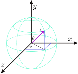
Figure 1: (Color online) Cartesian coordinate ($x,y,z$) and spherical coordinate ($r,\theta,\phi$) with $r$ the radial distance, $\theta$ the polar angle, and $\phi$ the azimuthal angle.

Although at this point $g(\theta)$ is an arbitrary function, it is natural to assume that it is associated with the solutions of the 2D Hemholtz equation. The procedure is that we first specify solutions of the 2D Helmholtz equation in different coordinates, and then construct an appropriate angular spectrum function $g(\theta)$. The corresponding Hemholtz wave eqution is of the form:

$$\left(\frac{\partial^{2}}{\partial z^{2}}+\frac{\partial^{2}}{\partial x^{2}}+k^{2}\right)f(z,x)=0,$$ (3)

the solutions of which include many functions – the exponential plane wave functions, Bessel functions, Mathieu functions, and Weber functions that can be expressed in the Cartesian, circular cylindrical, elliptic cylindrical, and parabolic cylindrical coordinates [33, 34, 35], respectively. Here $k^{2}$ is the eignevalue of the corresponding Laplace operator’s boundary value problem (connected with the wavenumber of the corresponding solutions). In the following sections, we will investigate the three cases for which the angular spectra are given in forms of the Mathieu and Weber functions, and the Fresnel integrals, respectively.

3 Mathieu beams

In the elliptic cylindrical coordinates $z=h\cosh\xi\cos\eta$ and $x=h\sinh\xi\sin\eta$, with $\xi\in[0,+\infty)$ and $\eta\in[0,2\pi)$, the solutions of the Helmholtz equation are the Mathieu functions. By utilizing variable separation, that is, by writing the solution of Eq. (3) as $f(\xi,\eta)=R(\xi)\Phi(\eta)$, Hemholtz equation separates into two ordinary differential equations [33, 35]

$$\frac{\partial^{2}R(\xi)}{\partial\xi^{2}}-(a-2q\cosh 2\xi)R(\xi)= 0,$$ (4a)

$$\frac{\partial^{2}\Phi(\eta)}{\partial\eta^{2}}+(a-2q\cos 2\eta)\Phi(\eta)= 0.$$ (4b)

where $a$ is the separation constant, $q=k^{2}h^{2}/4$ is a parameter related to the ellipticity of the coordinate system, $h$ is the interfocal separation, and $k=2\pi/\lambda$ is the wave number ($\lambda$ being the wavelength in the medium). The solutions of Eqs. (4a) and (4b) are the radial and angular Mathieu functions, respectively. A number of such solutions is known [35].

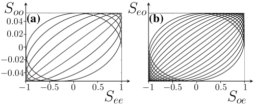
Figure 2: (a) Angular spectrum function $g_{1}(\theta)$. (b) Angular spectrum function $g_{2}(\theta)$. The order of the Mathieu functions is 10, and $q=4$.

We utilize the angular Mathieu functions to construct the corresponding spectral function $g$. Generally, there are four categories of the angular Mathieu solutions of Eq. (4b), denoted as $S_{ee},~{}S_{eo},~{}S_{oe}$, and $S_{oo}$ for the even-even, even-odd, odd-even, and odd-odd cases, respectively; they have been discussed in detail in [35]. They also carry an order $m$, which can be quite high in the cases considered here; the solutions then look quite similar and for convenience we suppress the order index $m$. Thus, the term $g(\theta)$ in the angular spectrum of Eq. (2) may be written in the following way:

$$g_{1}(\theta) =S_{ee}(\theta)+iS_{oo}(\theta),$$ (5)

$$g_{2}(\theta) =S_{oe}(\theta)+iS_{eo}(\theta),$$ (6)

and in this manner one may introduce the novel Mathieu accelerating beams, by utilizing the transverse Whittaker integral. This is in difference to the Mathieu nonparaxial beams introduced elsewhere [25], where combinations of the radial and angular Mathieu functions have been utilized. Before going to details, we show the angular spectrum functions $g_{1}$ and $g_{2}$ in Figs. 2(a) and 2(b). The order of the involved Mathieu functions is 10, with $q=4$.

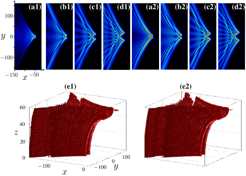
Figure 3: (Color online) Cross-section in the $z=0$ plane of the amplitude $|\psi(\bf r)|$ of the shape-invariant Mathieu beams with $q=4$ and $m=50$. The 1st, 4th, 7th, and 10th order Mathieu functions are displayed from left to right. (a1)-(d1) The case of $g_{1}$. (a2)-(d2) The case of $g_{2}$. (e1) and (e2) 3D plots of the propagating 10th Mathieu beam, corresponding to $g_{1}$ and $g_{2}$, respectively.

Based on the spectral functions $g_{1}$ and $g_{2}$, we display the transverse $|\psi(\bf r)|$ distributions of the shape-invariant Mathieu beams at $z=0$ in Figs. 3(a1)-3(d1) and Figs. 3(a2)-3(d2), respectively. It is seen that the amplitude distributions $|\psi(\bf r)|$ of the beams in the $z=0$ plane are symmetric about $y=0$, and that they become quite complex as the order is increased. Different from the $g_{1}$ case, the amplitude $|\psi(\bf r)|$ at the $y=0$ plane is always the smallest for the $g_{2}$ case. To observe the accelerating properties as the beams propagate, we choose the 10th order Mathieu functions as an example; numerical simulations are shown in Figs. 3(e1) and 3(e2), which correspond to the cases presented in Figs. 3(d1) and 3(d2), respectively. It is seen that the beams are almost invariant along the $z$ direction, slowly expanding and accelerating along a quarter-circular trajectory. Note that the beams mirror-extend below the $z=0$ plane, so that the beams in the $y=const$ plane accelerate along a semicircular trajectory. This comes from the following argument.

As indicated in Sec. 2, we set the polar angle $\phi$ in the interval $[-\pi/2,~{}\pi/2]$; that means the beam propagates in the positive $z$ direction. If $\phi\in[\pi/2,~{}3\pi/2]$, the beam will propagate in the negative $z$ direction, and it will also accelerate along a quarter-circular trajectory, which is symmetric about the plane $z=0$ to the positive quarter-circular trajectory. When both the positively and negatively propagating beams are considered together, one observes a beam accelerating along a semicircular trajectory. For convenience, we only consider the case of $\phi\in[-\pi/2,~{}\pi/2]$ throughout the Letter. From the 3D plot of the acceleration process, we see that the beams exhibit a nonparaxial accelerating property during propagation – as they should.

4 Weber beams

The solutions of the Helmholtz equations in the parabolic cylindrical coordinates are the Weber functions. The relation between the Cartesian and parabolic cylindrical coordinates is $z+ix=(\xi+i\eta)^{2}/2$, with $\xi\in[0,+\infty)$ and $\eta\in(-\infty,+\infty)$. When Eq. (3) is expressed in the parabolic cylindrical coordinates, and the method of separation of variables applied, the Hemholtz equation is transformed into a system of equations [25, 34, 35]

$$\frac{\partial^{2}R(\xi)}{\partial\xi^{2}}+\left(k^{2}\xi^{2}-2ka\right)R(\xi)= 0,$$ (7a)

$$\frac{\partial^{2}\Phi(\eta)}{\partial\eta^{2}}+\left(k^{2}\eta^{2}+2ka\right)\Phi(\eta)= 0,$$ (7b)

in which $2ka$ is the separation constant. If one sets $\sqrt{2k}\xi=u$ and $\sqrt{2k}\eta=v$, Eqs. (7a) and (7b) transform into the two standard Weber’s differential equations

$$\frac{\partial^{2}R(u)}{\partial u^{2}}+\left(\frac{u^{2}}{4}-a\right)R(u)= 0,$$ (8a)

$$\frac{\partial^{2}\Phi(v)}{\partial v^{2}}+\left(\frac{v^{2}}{4}+a\right)\Phi(v)= 0.$$ (8b)

Therefore, the solutions of Eqs. (7a) and (7b) are the Weber functions with different eigenvalues. If we denote the even and odd solutions of Eq. (7b) as $P_{e}$ and $P_{o}$, we can define the angular spectrum function $g(\theta)$ as

$$g(\theta)=P_{e}(\theta,a)+iP_{o}(\theta,a),$$ (9)

in which

$$P_{e,o}(\theta,a)= \sum^{\infty}_{n=0}c_{n}\frac{\theta^{n}}{n!},$$ (10a)

and the coefficients $$c_{n}$$ satisfy the following recurrence relation:

$$c_{n+2}= ac_{n}-\frac{n(n-1)c_{n-2}}{4}.$$ (10b)

To obtain $P_{e}$ or $P_{o}$, one sets the first two $c_{n}$ coefficients to $c_{0}=1,c_{1}=0$ or to $c_{0}=0,c_{1}=1$, respectfully [34]. This choice for the angular spectrum functions is again different from the choice made in [25], in which the combinations of solutions of both Eqs. (7a) and (7b) are used to construct the full angular spectrum of Weber accelerating beams. These Weber beams accelerate along parabolic trajectories and are different from the ones introduced here.

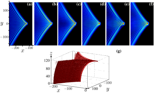
Figure 4: (Color online) (a)-(f) Wave amplitude $|\psi(\bf r)|$ distribution at $z=0$ of the shape-invariant Weber beams, for $m=120$ and $a=1,~{}7,~{}10,~{}13,~{}16$ and $19$, respectively. (g) 3D plot of the Weber beam with $a=1$.

To display our Weber beams, we repeat the same procedure as for the Mathieu beams; the only difference is that now there are not two $g$ functions but one, expressed in terms of the even and odd Weber eigenfunctions. The amplitude $|\psi(\bf r)|$ distribution of Weber beams at $z=0$ for $m=120$ and different $a$, according to Eqs. (9) and (10), is shown in Figs. 4(a)-4(f). It is seen that the $|\psi(\bf r)|$ distribution changes slightly with $a$ increasing, especially around the point $(x=-m,~{}y=0)$. Regardless of what the $|\psi(\bf r)|$ distribution at the $z=0$ plane is, the beam still accelerates along a quarter-circular trajectory. As an example, Fig. 4(g) depicts the accelerating process of the beam with $a=1$, which corresponds to Fig. 4(a). It is clear that the shape of the beam is nearly invariant as it propagates, and the accelerating trajectory is a quarter of the full circle in the plane $y=0$ (the bending angle is approximately $90^{\circ}$). So, the acceleration is nonparaxial.

5 Fresnel integrals

In optics, Fresnel integrals are commonly used to describe Fresnel diffraction from a straight edge or a rectangular aperture. The Fresnel cosine and sine integrals are defined as [36]

$$\mathcal{C}(t)= \int^{t}_{0}\cos\left(\frac{\pi}{2}\tau^{2}\right)d\tau,$$ (11a)

$$\mathcal{S}(t)= \int^{t}_{0}\sin\left(\frac{\pi}{2}\tau^{2}\right)d\tau,$$ (11b)

or in the complex form:

$$\mathcal{F}(t)=\mathcal{C}(t)+i\mathcal{S}(t).$$ (12)

Thus, we define the new Fresnel nonparaxial accelerating wave by introducing the spectrum function $g(\theta)$ as

$$g(\theta)=\left(\mathcal{C}(\theta)+\frac{1}{2}\right)+i\left(\mathcal{S}(\theta)+\frac{1}{2}\right).$$ (13)

These Fresnel waves are different from the ones introduced in [9], which propagate paraxially along parabolic trajectories. The spectral function $g(\theta)$ is shown in Fig. 5(a), which is the Cornu spiral [36]; the two branches of the spiral approach the points $P_{1}$ and $P_{2}$, with the coordinates $(1/\sqrt{2},1/\sqrt{2})$ and $(0,0)$.

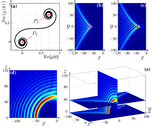
Figure 5: (Color online) (a) Spectrum function $g(\theta)$ of Fresnel integrals. (b) Transverse intensity distribution of the beam with $m=50$ at $z=0$. (c) Same as (b) but at $z=40$. (d) Acceleration along the circular trajectory of the beam at the cross-section at the plane $y=0$. (e) The panels (c), (d) and (e) put together.

According to Eq. (13) and the Whittaker integral, we can now present the Fresnel nonparaxial accelerating beams. We display the intensity distributions of the accelerating beam at $z=0$ plane, $z=40$ plane, and $y=0$ plane in Figs. 5(b), 5(c), and 5(d), respectively. Concerning the intensity at $z=0$ plane, it is similar to the ones shown in Figs. 3(a1) and 4(a), even though the angular spectra are quite different. In comparison with Figs. 5(b) and 5(c), we find the beam accelerating – all the lobes move rightward along the positive $x$ direction. In Fig. 5(d) we can follow the acceleration of the main lobe and other higher-order lobes in the $y=0$ plane. It is evident that the lobes accelerate along a quarter-circular trajectory, with a bending angle $\sim 90^{\circ}$, which demonstrates that the acceleration is nonparaxial. As before, the beams in Fig. 5(d) extend to the region $z\leq 0$, so that the acceleration actually proceeds along semicircular trajectories. In order to see the accelerating process more clearly, we put Figs. 5(b), 5(c) and 5(d) together in Fig. 5(e).

6 Conclusion

Based on the transverse Whittaker integral, we have investigated the novel 3D nonparaxial accelerating beams, by constructing the angular spectra using Mathieu functions, Weber functions, and Fresnel integrals, respectively. In the transverse plane, the intensity distributions of the accelerating beams are related to the angular spectra. In the longitudinal direction, the beams accelerate along a quarter-circular trajectory, with the bending angle approximately $90^{\circ}$. Even though the angular Mathieu functions, Weber functions, and Fresnel integrals used here are not strictly rotationally symmetric, investigation on such 3D nonparaxial accelerating beams is still meaningful and deserves appropriate attention. Since Mathieu and Weber functions are the solutions of the Helmholtz equation, and the Fresnel integrals are used to describe optical diffraction, which are all related to common phenomena in real world, we hope to have revealed the importance of such beams for potential applications.

References

- [1] Georgios A. Siviloglou and Demetrios N. Christodoulides. Accelerating finite energy Airy beams. Opt. Lett., 32(8):979–981, Apr 2007.
- [2] G. A. Siviloglou, J. Broky, A. Dogariu, and D. N. Christodoulides. Observation of accelerating Airy beams. Phys. Rev. Lett., 99:213901, Nov 2007.
- [3] Miguel A. Bandres and Julio C. Gutiérrez-Vega. Airy-Gauss beams and their transformation by paraxial optical systems. Opt. Express, 15(25):16719–16728, Dec 2007.
- [4] Tal Ellenbogen, Noa Voloch-Bloch, Ayelet Ganany-Padowicz, and Ady Arie. Nonlinear generation and manipulation of Airy beams. Nat. Photon., 3(7):395–398, 2009.
- [5] Andy Chong, William H Renninger, Demetrios N Christodoulides, and Frank W Wise. Airy-Bessel wave packets as versatile linear light bullets. Nat. Photon., 4(2):103–106, 2010.
- [6] Nikolaos K. Efremidis and Demetrios N. Christodoulides. Abruptly autofocusing waves. Opt. Lett., 35(23):4045–4047, Dec 2010.
- [7] T. J. Eichelkraut, G. A. Siviloglou, I. M. Besieris, and D. N. Christodoulides. Oblique Airy wave packets in bidispersive optical media. Opt. Lett., 35(21):3655–3657, Nov 2010.
- [8] Yiqi Zhang, Milivoj Belić, Zhenkun Wu, Huaibin Zheng, Keqing Lu, Yuanyuan Li, and Yanpeng Zhang. Soliton pair generation in the interactions of Airy and nonlinear accelerating beams. Opt. Lett., 38(22):4585–4588, Nov 2013.
- [9] Yiqi Zhang, Milivoj R. Belić, Huaibin Zheng, Zhenkun Wu, Yuanyuan Li, Keqing Lu, and Yanpeng Zhang. Fresnel diffraction patterns as accelerating beams. Europhys. Lett., 104(3):34007, 2013.
- [10] Yiqi Zhang, Milivoj R. Belić, Huaibin Zheng, Haixia Chen, Changbiao Li, Yuanyuan Li, and Yanpeng Zhang. Interactions of Airy beams, nonlinear accelerating beams, and induced solitons in Kerr and saturable nonlinear media. Opt. Express, 22(6):7160–7171, Mar 2014.
- [11] M. V. Berry and N. L. Balazs. Nonspreading wave packets. Am. J. Phys., 47:264–267, 1979.
- [12] J. Durnin. Exact solutions for nondiffracting beams. I. the scalar theory. J. Opt. Soc. Am. A, 4(4):651–654, Apr 1987.
- [13] J. Durnin, J. J. Miceli, and J. H. Eberly. Diffraction-free beams. Phys. Rev. Lett., 58:1499–1501, Apr 1987.
- [14] John Broky, Georgios A. Siviloglou, Aristide Dogariu, and Demetrios N. Christodoulides. Self-healing properties of optical Airy beams. Opt. Express, 16(17):12880–12891, Aug 2008.
- [15] Yi Hu, Simon Huang, Peng Zhang, Cibo Lou, Jingjun Xu, and Zhigang Chen. Persistence and breakdown of Airy beams driven by an initial nonlinearity. Opt. Lett., 35(23):3952–3954, Dec 2010.
- [16] Ido Kaminer, Mordechai Segev, and Demetrios N. Christodoulides. Self-accelerating self-trapped optical beams. Phys. Rev. Lett., 106:213903, May 2011.
- [17] Nikolaos K. Efremidis, Vassilis Paltoglou, and Wolf von Klitzing. Accelerating and abruptly autofocusing matter waves. Phys. Rev. A, 87:043637, Apr 2013.
- [18] Alexander Minovich, Angela E. Klein, Norik Janunts, Thomas Pertsch, Dragomir N. Neshev, and Yuri S. Kivshar. Generation and near-field imaging of Airy surface plasmons. Phys. Rev. Lett., 107:116802, Sep 2011.
- [19] L. Li, T. Li, S. M. Wang, C. Zhang, and S. N. Zhu. Plasmonic Airy beam generated by in-plane diffraction. Phys. Rev. Lett., 107:126804, Sep 2011.
- [20] Lin Li, Tao Li, Shuming Wang, Shining Zhu, and Xiang Zhang. Broad band focusing and demultiplexing of in-plane propagating surface plasmons. Nano Lett., 11(10):4357–4361, 2011.
- [21] Fei Zhuang, Jianqi Shen, Xinyue Du, and Daomu Zhao. Propagation and modulation of Airy beams through a four-level electromagnetic induced transparency atomic vapor. Opt. Lett., 37(15):3054–3056, Aug 2012.
- [22] Fei Zhuang, Xinyue Du, Yuqian Ye, and Daomu Zhao. Evolution of Airy beams in a chiral medium. Opt. Lett., 37(11):1871–1873, Jun 2012.
- [23] Ido Kaminer, Jonathan Nemirovsky, Konstantinos G. Makris, and Mordechai Segev. Self-accelerating beams in photonic crystals. Opt. Express, 21(7):8886–8896, Apr 2013.
- [24] Parinaz Aleahmad, Mohammad-Ali Miri, Matthew S. Mills, Ido Kaminer, Mordechai Segev, and Demetrios N. Christodoulides. Fully vectorial accelerating diffraction-free Helmholtz beams. Phys. Rev. Lett., 109:203902, Nov 2012.
- [25] Peng Zhang, Yi Hu, Tongcang Li, Drake Cannan, Xiaobo Yin, Roberto Morandotti, Zhigang Chen, and Xiang Zhang. Nonparaxial Mathieu and Weber accelerating beams. Phys. Rev. Lett., 109:193901, Nov 2012.
- [26] Ido Kaminer, Rivka Bekenstein, Jonathan Nemirovsky, and Mordechai Segev. Nondiffracting accelerating wave packets of Maxwell’s equations. Phys. Rev. Lett., 108:163901, Apr 2012.
- [27] Miguel A Bandres and B M Rodríguez-Lara. Nondiffracting accelerating waves: Weber waves and parabolic momentum. New J. Phys., 15(1):013054, 2013.
- [28] Edmund Taylor Whittaker and George Neville Watson. A course of modern analysis. Cambridge University Press, Cambridge, 4 edition, 1996.
- [29] Miguel A. Alonso and Miguel A. Bandres. Spherical fields as nonparaxial accelerating waves. Opt. Lett., 37(24):5175–5177, Dec 2012.
- [30] Le-Wei Li, Mook-Seng Leong, Tat-Soon Yeo, Pang-Shyan Kooi, and Kian-Yong Tan. Computations of spheroidal harmonics with complex arguments: A review with an algorithm. Phys. Rev. E, 58:6792–6806, Nov 1998.
- [31] Miguel A. Bandres, Miguel A. Alonso, Ido Kaminer, and Mordechai Segev. Three-dimensional accelerating electromagnetic waves. Opt. Express, 21(12):13917–13929, Jun 2013.
- [32] E Wolf. Electromagnetic diffraction in optical systems. I. an integral representation of the image field. Proc. Roy. Soc. A., 253(1274):349–357, 1959.
- [33] J. C. Gutiérrez-Vega, M. D. Iturbe-Castillo, and S. Chávez-Cerda. Alternative formulation for invariant optical fields: Mathieu beams. Opt. Lett., 25(20):1493–1495, Oct 2000.
- [34] Miguel A. Bandres, Julio C. Gutiérrez-Vega, and Sabino Chávez-Cerda. Parabolic nondiffracting optical wave fields. Opt. Lett., 29(1):44–46, Jan 2004.
- [35] Milton Abramowitz and Irene A Stegun. Handbook of Mathematical Functions. Dover Publications Inc., New York, 1970.
- [36] Max Born and Emil Wolf. Principles of Optics. Cambridge University Press, Cambridge, 7 edition, 1999.