Temperature Dependence of the Spin Susceptibility in
Noncentrosymmetric Superconductors with Line Nodes

Abstract

The spin susceptibility of noncentrosymmetric superconductors is studied when the gap function has line nodes. As examples, d-wave states, where the gap function has an additional odd-parity phase factor, are examined. The curve of the spin susceptibility $\chi(T)$ is upward convex when all line nodes are parallel to the magnetic field, while it is downward convex in the other d-wave states and an s-wave state. For polycrystalline powder samples, the temperature dependences of $\chi(T)$ are predicted by assuming three explicit conditions of the powder particles. The results are compared with the experimental data of the Knight shift observed in ${\rm Li_{2}Pt_{3}B}$ and ${\rm Li_{2}Pd_{3}B}$.

1 Introduction

Noncentrosymmetric superconductors ${\rm Li_{2}Pt_{3}B}$ and ${\rm Li_{2}Pd_{3}B}$ exhibit quite different superconductivity behavior despite the similarity of their chemical and crystal structures. The superconducting transition temperature ${T_{\rm c}}$ is 7 K for ${\rm Li_{2}Pd_{3}B}$ [1], while it is 2.7 K for ${\rm Li_{2}Pt_{3}B}$ [2]. Regarding the pairing anisotropy, most of the experimental results, such as the temperature dependences of the nuclear magnetic relaxation (NMR) rate $T_{1}^{-1}$ [3, 4], magnetic penetration depth [5], and specific heat [6, 7], indicate that the gap function has no nodes in ${\rm Li_{2}Pd_{3}B}$, while it has line nodes in ${\rm Li_{2}Pt_{3}B}$, although the $H$–$T$ phase diagram for ${\rm Li_{2}(Pd_{1-x}Pt_{x})_{3}B}$ is qualitatively unchanged for $0\leq x\leq 1$ [8]. The temperature dependence of the Knight shift observed by Nishiyama et al. [3, 4] indicates a full-gap state for ${\rm Li_{2}Pd_{3}B}$, which is consistent with the above experiments, while for ${\rm Li_{2}Pt_{3}B}$, the interpretation of the temperature dependence is nontrivial.

In ${\rm Li_{2}Pt_{3}B}$, the Knight shift remains unchanged below ${T_{\rm c}}$ within experimental resolution [3, 4], which indicates that the spin susceptibility is not reduced by the growth of the superconducting gap. Therefore, this implies that the superconducting state does not contain Cooper pairs of antiparallel-spin electrons, where the spin quantization axis is parallel to the magnetic field. However, such a superconducting state that consists purely of parallel-spin pairs cannot occur in systems with strong spin-orbit coupling, except in rare situations.

To discuss this issue, let us consider the bilinear terms of the Hamiltonian

$$H_{0}=\sum_{{{\bm{k}}}}\sum_{\sigma_{1}\sigma_{2}}c_{{{\bm{k}}}\sigma_{1}}^{\dagger}\Bigl{[}\xi_{{{\bm{k}}}}^{0}\,\sigma_{0}-\alpha_{{{\bm{k}}}}\,{\hat{{{\bm{g}}}}}({{\bm{k}}})\cdot\bm{\sigma}\Bigr{]}_{\sigma_{1}\sigma_{2}}c_{{{\bm{k}}}\sigma_{2}},$$ (1)

where $\sigma_{0}$, $\bm{\sigma}$, and $c_{{{\bm{k}}}\sigma}$ are the $2\times 2$ identity matrix, the Pauli matrices, and the annihilation operator of the electron with momentum ${{\bm{k}}}$ and spin $\sigma$, respectively. The vector function ${\hat{{\bm{g}}}}({{\bm{k}}})$ is assumed to satisfy ${\hat{{\bm{g}}}}(-{{\bm{k}}})=-{\hat{{\bm{g}}}}({{\bm{k}}})$ and $|{\hat{{\bm{g}}}}({{\bm{k}}})|=1$. We introduce the polar coordinates $({\bar{\theta}}_{{{\bm{k}}}},{\bar{\varphi}}_{{{\bm{k}}}})$ for the direction of ${\hat{{\bm{g}}}}({{\bm{k}}})$ by

$$\begin{split}{\hat{{\bm{g}}}}({{\bm{k}}})&=(g_{x}({{\bm{k}}}),g_{y}({{\bm{k}}}),g_{z}({{\bm{k}}}))\\ &=(\sin{\bar{\theta}}_{{{\bm{k}}}}\cos{\bar{\varphi}}_{{{\bm{k}}}},\sin{\bar{\theta}}_{{{\bm{k}}}}\sin{\bar{\varphi}}_{{{\bm{k}}}},\cos{\bar{\theta}}_{{{\bm{k}}}}),\end{split}$$ (2)

where the $z$-axis lies along the magnetic field direction. $H_{0}$ is diagonalized by a unitary transformation of the electron operators in spin space [9, 10, 11, 12], leading to the spin-orbit split bands having the one-particle energies ${\tilde{\xi}}_{{{\bm{k}}}s}=\xi_{{{\bm{k}}}}^{0}-s\alpha_{{{\bm{k}}}}$, where $s=\pm$. With $c_{{{\bm{k}}}\sigma}$ and the annihilation operator ${\tilde{c}}_{{{\bm{k}}}s}$ of the electron with momentum ${{\bm{k}}}$ in the $s$-band, the superconducting order parameters are written as $\psi_{\sigma\sigma^{\prime}}({{\bm{k}}})=\langle c_{{{\bm{k}}}\sigma}c_{-{{\bm{k}}}\sigma^{\prime}}\rangle$ and ${\tilde{\psi}}_{ss^{\prime}}({{\bm{k}}})=\langle{\tilde{c}}_{{{\bm{k}}}s}{\tilde{c}}_{-{{\bm{k}}}s^{\prime}}\rangle$. The former is expressed as $\psi_{\uparrow\uparrow}=-d_{x}+id_{y}$, $\psi_{\downarrow\downarrow}=d_{x}+id_{y}$, $\psi_{\uparrow\downarrow}=d_{z}+d_{0}$, and $\psi_{\downarrow\uparrow}=d_{z}-d_{0}$, in terms of the d-vector ${{\bm{d}}}({{\bm{k}}})=(d_{x}({{\bm{k}}}),d_{y}({{\bm{k}}}),d_{z}({{\bm{k}}}))$ and the singlet component $d_{0}({{\bm{k}}})$ of the order parameter.

When $\alpha_{{{\bm{k}}}}\gg{k_{\rm B}}{T_{\rm c}}$, the spin-orbit splitting of the Fermi-surfaces is so large that interband pairing does not occur, that is, ${\tilde{\psi}}_{\pm\mp}({{\bm{k}}})=0$. This immediately leads to ${{\bm{d}}}({{\bm{k}}})\parallel{\hat{{{\bm{g}}}}}({{\bm{k}}})$ as Frigeri et al. discovered [13]. In this case, we can define a scalar function $d({{\bm{k}}})$ by

$${{\bm{d}}}({{\bm{k}}})=d({{\bm{k}}}){\hat{{{\bm{g}}}}}({{\bm{k}}}),$$ (3)

leading to

$${\tilde{\psi}}_{ss}({{\bm{k}}})=s_{{{\bm{k}}}}(d({{\bm{k}}})+sd_{0}({{\bm{k}}})),$$ (4)

where $s_{{{\bm{k}}}}$ is an odd-parity phase factor that originates from the unitary transformation [9, 10, 12]. From the Knight shift data in ${\rm Li_{2}Pt_{3}B}$ mentioned above, if we assume that antiparallel-spin pairing is suppressed, $\psi_{\uparrow\downarrow}({{\bm{k}}})=\psi_{\downarrow\uparrow}({{\bm{k}}})=0$, i.e., $d_{0}({{\bm{k}}})=d_{z}({{\bm{k}}})=0$, it follows that $d({{\bm{k}}})=0$ from Eq. (3) unless ${\hat{g}}_{z}({{\bm{k}}})=0$. Hence, all components of the superconducting order parameter vanish, that is, $d_{0}({{\bm{k}}})=0$ and ${{\bm{d}}}({{\bm{k}}})=0$. Therefore, pure parallel-spin pairing can occur over regions of ${{\bm{k}}}$’s that satisfy the conditions ${\bar{\theta}}_{{{\bm{k}}}}\approx\pi/2$ or $\alpha_{{{\bm{k}}}}\approx 0$.

It seems unusual that such a limited region has a sufficiently large density of states to yield the observed transition temperature. Even if this was possible in single crystal samples for an appropriate magnetic field direction, such a condition of the magnetic field direction is not satisfied in polycrystalline powder samples in which the orientation of each powder particle is random. Therefore, the interpretation of the Knight shift data for ${\rm Li_{2}Pt_{3}B}$ appears problematic. However, this difficulty can be resolved as we shall examine below, if we assume that the system is affected by the applied magnetic field.

In Eq. (4), $d({{\bm{k}}})$ and $d_{0}({{\bm{k}}})$ are of even parity from their definitions. Therefore, if parity-mixing terms are ignored in pairing interactions, the gap function is expanded as

$$\Delta_{{{\bm{k}}}s}=s_{{{\bm{k}}}}\sum_{\alpha({\rm even})}\Delta_{\alpha}^{(s)}\gamma_{\alpha}^{(s)}({{\bm{k}}}),$$ (5)

with basis functions $\gamma_{\alpha}^{(s)}({{\bm{k}}})$, where $\alpha$ denotes the symmetry index and the summation is taken over $\alpha$’s of even parity. For example, $\alpha=(l,m)$ is convenient in spherically symmetric systems, where $l$ and $m$ are the quantum numbers of angular momentum. Since the phase factor $s_{{{\bm{k}}}}$ has nothing to do with the quasi-particle energy $E_{{{\bm{k}}}s}=\sqrt{{\tilde{\xi}}_{{{\bm{k}}}s}^{2}+|\Delta_{{{\bm{k}}}s}|^{2}}$, it is appropriate to index the gap function by the value of $\alpha$ that is dominant in the summation in Eq. (5). Therefore, the lowest-order line-node state is a d-wave [12].

An interesting problem to consider is how the difference in the superconductivity between ${\rm Li_{2}Pd_{3}B}$ and ${\rm Li_{2}Pt_{3}B}$ arises in spite of their similarity. This difference can be attributed to differences in the pairing interactions and the one-particle dispersion energy [12]. In the case that those differences originate from differences in the strength of the spin-orbit interactions, a transition between a full-gap state and a line-node state would occur if we could continuously increase the spin-orbit coupling constant between the two compounds.

Shishidou and Oguchi have obtained spin-orbit split Fermi-surfaces for these compounds by first-principles calculations [14]. Their results suggest that every Fermi surface has a spin-orbit split partner in ${\rm Li_{2}Pd_{3}B}$, while in ${\rm Li_{2}Pt_{3}B}$, many of the Fermi surfaces do not have partners because of stronger spin-orbit coupling.

In our previous work [12], we proposed a scenario in which the disappearance of one of the spin-orbit split Fermi surfaces in ${\rm Li_{2}Pt_{3}B}$ is mainly responsible for the difference observed in the superconductivity. Examining several types of pairing interactions, it was found that, when a charge–charge interaction is dominant, the transition from a full-gap state to a line-node state occurs over a wide and realistic region of the parameter space of the coupling constants for the interaction with increasing the spin-orbit coupling constant. If this scenario holds for the present compounds, presumably an s-wave nearly-spin-triplet state and a d-wave mixed-singlet-triplet state are realized in ${\rm Li_{2}Pd_{3}B}$ and ${\rm Li_{2}Pt_{3}B}$, respectively. These states are consistent with most of the available experimental data. For the Knight shifts in the superconducting states, the temperature dependence observed in ${\rm Li_{2}Pd_{3}B}$ can be understood by assuming an s-wave state, independently of the weights of the spin-singlet and triplet components, as shown below, while in ${\rm Li_{2}Pt_{3}B}$ it is nontrivial, as explained above.

In the present work, we examine the temperature dependence of the spin susceptibility for noncentrosymmetric superconductors, when the gap function has line nodes. We discuss a scenario in which the temperature dependences of the Knight shifts are consistently reproduced for ${\rm Li_{2}Pd_{3}B}$ and ${\rm Li_{2}Pt_{3}B}$, assuming s-wave and d-wave states, respectively, without specifying the microscopic origin of the pairing interactions. This assumption is phenomenologically plausible from the experimental results mentioned above, and consistent with the scenario proposed in our previous paper. [12]

The spin susceptibility of noncentrosymmetric superconductors has been studied by many authors [15, 16, 9, 17, 18, 19, 20, 21, 22, 23]. In particular, it has been found that the spin susceptibility has a large Van Vleck component $\chi_{\rm V}$ that is almost temperature independent in the superconducting phase [9, 17, 18, 19, 20, 21, 22, 23].

The behavior of the Knight shift in ${\rm Li_{2}Pt_{3}B}$ implies that the difference in the spin susceptibilities $\Delta\chi\equiv\chi_{\rm N}-\chi_{\rm S}$ is small, where the subscripts N and S denote the normal and superconducting phases, respectively. Maruyama and Yanase obtained $\Delta\chi/\chi_{\rm N}=1-\chi_{\rm S}/\chi_{\rm N}<0.1$, which is consistent with the experimental results for ${\rm Li_{2}Pt_{3}B}$, considering the reduction of the density of states for ${\rm Li_{2}Pt_{3}B}$ because of stronger spin-orbit coupling [23].

This small value of $\Delta\chi/\chi_{\rm N}$ is obtained by considering the large Van Vleck component $\chi_{\rm V}$, which significantly reduces the ratio $\Delta\chi/\chi_{\rm N}$. However, concerning the comparison of two compounds, the relevant quantity is the ratio $\Delta\chi^{\rm Pt}/\Delta\chi^{\rm Pd}$ rather than the ratio $\Delta\chi^{\rm Pt}/\chi_{\rm N}^{\rm Pt}$, where the superscripts Pt and Pd represent ${\rm Li_{2}Pt_{3}B}$ and ${\rm Li_{2}Pd_{3}B}$ systems, respectively. The Van Vleck component $\chi_{\rm V}$ would not significantly change the ratio $\Delta\chi^{\rm Pt}/\Delta\chi^{\rm Pd}$ because it would reduce both $\Delta\chi^{\rm Pt}$ and $\Delta\chi^{\rm Pd}$ to a similar extent. Therefore, it seems that the smallness of $\Delta\chi^{\rm Pt}/\Delta\chi^{\rm Pd}$ observed by the Knight shift measurement is not completely explained only by the reduction of the density of states. Moreover, if $\Delta\chi^{\rm Pt}/\Delta\chi^{\rm Pd}$ is small merely because of the small density of states, ${T_{\rm c}}$ should be negligibly small in ${\rm Li_{2}Pt_{3}B}$ in comparison to that in ${\rm Li_{2}Pd_{3}B}$, unless the pairing interaction is extremely strong in ${\rm Li_{2}Pt_{3}B}$.

In Sect. 2, an expression for the spin susceptibility is presented. In Sect. 3, the spin susceptibilities are numerically calculated for various d-wave states using a simplified model. The results are compared with Knight shift data [4] for ${\rm Li_{2}Pd_{3}B}$ and ${\rm Li_{2}Pt_{3}B}$. The final section summarizes the results.

2 Formulation

We briefly review the expression for the spin susceptibility to clarify the notation. The total magnetization is expressed as ${M=\mu_{\rm e}\langle{\hat{m}}\rangle}$ with

$${\hat{m}}=\sum_{i}\sum_{\sigma,\sigma^{\prime}}c_{i\sigma}^{\dagger}\sigma_{\sigma\sigma^{\prime}}^{z}c_{i\sigma^{\prime}},$$ (6)

where the index $i$ denotes the lattice site, and $\mu_{\rm e}$ is the electron magnetic moment. The Zeeman energy term of the Hamiltonian is $H_{m}=-\mu_{\rm e}H{\hat{m}}$, for a magnetic field ${{\bm{H}}}=(0,0,H)$. The spin susceptibility per site is calculated by the formula:

$$\chi=i\int_{0}^{\infty}dt\,\,\frac{1}{N}\langle[{\hat{m}}(t),{\hat{m}}(0)]\rangle.$$ (7)

In the superconducting state, the spin susceptibility is obtained as $\chi=\chi_{1}+\chi_{2}+\chi_{3}$, where

$$\chi_{1}=\frac{1}{N}\sum_{{{\bm{k}}},s}\cos^{2}{\bar{\theta}}_{{{\bm{k}}}}\,\Bigl{[}-\frac{d}{dE}f(E)\Bigr{]}_{E=E_{{{\bm{k}}}s}},$$ (8)

$$\chi_{2}=-\frac{2}{N}\sum_{{{\bm{k}}}}\sin^{2}{\bar{\theta}}_{{{\bm{k}}}}\,\Bigl{[}n_{+-}({{\bm{k}}})\Bigr{]}^{2}\,\frac{f(E_{{{\bm{k}}}+})-f(E_{{{\bm{k}}}-})}{E_{{{\bm{k}}}+}-E_{{{\bm{k}}}-}},$$ (9)

$$\chi_{3}=-\frac{2}{N}\sum_{{{\bm{k}}}}\sin^{2}{\bar{\theta}}_{{{\bm{k}}}}\,\Bigl{[}m_{+-}({{\bm{k}}})\Bigr{]}^{2}\,\frac{f(E_{{{\bm{k}}}+})-f(-E_{{{\bm{k}}}-})}{E_{{{\bm{k}}}+}+E_{{{\bm{k}}}-}},$$ (10)

and $n_{+-}({{\bm{k}}})=u_{{{\bm{k}}}+}u_{{{\bm{k}}}-}-v_{{{\bm{k}}}+}v_{{{\bm{k}}}-}$, $m_{+-}({{\bm{k}}})=u_{{{\bm{k}}}+}v_{{{\bm{k}}}-}+v_{{{\bm{k}}}+}u_{{{\bm{k}}}-}$, $u_{{{\bm{k}}}s}=\bigl{[}\bigl{(}1+{\tilde{\xi}}_{{{\bm{k}}}s}/E_{{{\bm{k}}}s}\bigr{)}/2\bigr{]}^{1/2}$, and $v_{{{\bm{k}}}s}=s\bigl{[}\bigl{(}1-{\tilde{\xi}}_{{{\bm{k}}}s}/E_{{{\bm{k}}}s}\bigr{)}/2\bigr{]}^{1/2}$.

When $\alpha_{{{\bm{k}}}}\gg|\Delta_{{{\bm{k}}}s}|$, the temperature dependence of the spin susceptibility mainly occurs from $\chi_{1}$, and the interband component $\chi_{2}+\chi_{3}=\chi_{\rm V}$ barely depends on the temperature [9, 17]. Therefore, the reduction of the spin susceptibility in the superconducting phase is $\Delta\chi\equiv\chi_{\rm N}-\chi_{\rm S}\approx\chi_{\rm 1N}-\chi_{\rm 1S}$. The difference in the Knight shifts between the superconducting and normal phases is expressed as $\Delta K=|A_{\rm hf}|\Delta\chi$ in terms of $\Delta\chi$ with the hyperfine coupling constant $A_{\rm hf}<0$ between the nuclear and electron spins. Since $\chi_{\rm N}$ and $\chi_{\rm 1N}$ are almost constant for the metals, and $\chi_{\rm 1S}(0)=0$, we obtain $\Delta\chi(0)=\chi_{1{\rm N}}=\langle\cos^{2}{\bar{\theta}}_{{{\bm{k}}}}\rangle_{\rm F}\chi_{\rm N}$, where $\langle\cdots\rangle_{\rm F}$ denotes the average over the Fermi surface. For example, in spherically symmetric systems, $\langle\cos^{2}{\bar{\theta}}_{{{\bm{k}}}}\rangle_{\rm F}=1/3$ and $\Delta\chi(0)=\chi_{\rm N}/3$ [9, 17]. In planar systems in which ${\hat{{\bm{g}}}}({{\bm{k}}})\perp{\hat{{\bm{z}}}}$ for all ${{\bm{k}}}$, $\langle\cos^{2}{\bar{\theta}}_{{{\bm{k}}}}\rangle_{\rm F}=0$ and $\Delta\chi(0)=0$, when ${{\bm{H}}}\parallel{\hat{{\bm{z}}}}$. In general, the ratio $\Delta\chi(0)/\chi_{\rm N}=\langle\cos^{2}{\bar{\theta}}_{{{\bm{k}}}}\rangle_{\rm F}$ is much smaller than the value 1 for centrosymmetric singlet superconductors. However, considering the similarity of the ${\rm Li_{2}Pd_{3}B}$ and ${\rm Li_{2}Pt_{3}B}$ crystal structures, the averages $\langle\cos^{2}{\bar{\theta}}_{{{\bm{k}}}}\rangle_{\rm F}$ for the two compounds would be roughly canceled out in $\Delta\chi^{\rm Pt}(0)/\Delta\chi^{\rm Pd}(0)$ at $T=0$.

At finite temperatures below ${T_{\rm c}}$, the temperature dependence of $\Delta\chi(T)$ differs qualitatively depending on the pairing anisotropy. As is well known, $\Delta\chi(T)$ is proportional to the Yosida function in the s-wave state, while it is proportional to $T$ at low temperatures in the line-node states. In addition to this difference, the factor $\cos^{2}{\bar{\theta}}_{{{\bm{k}}}}$ in $\chi_{1}$ gives rise to qualitatively different temperature dependences in the d-wave states for noncentrosymmetric superconductors. When the gap function has a peak near ${\bar{\theta}}_{{{\bm{k}}}}=\pi/2$, the growth of the superconducting gap is less effective at reducing the susceptibility $\chi_{1}$. As a result, the difference $\Delta\chi=\chi_{\rm N}-\chi_{\rm S}$ becomes smaller. Similarly, when the gap function has a peak near ${\bar{\theta}}_{{{\bm{k}}}}=0$ or $\pi$, the growth of the superconducting gap is more effective at reducing the susceptibility $\chi_{1}$, and the difference $\Delta\chi$ becomes larger.

To illustrate this phenomenon, we suppose a spherically symmetric system in which ${\hat{{\bm{g}}}}({{\bm{k}}})={{\bm{k}}}/|{{\bm{k}}}|\equiv{\hat{{\bm{k}}}}$. The basis functions are written as

$${\gamma_{lm}^{(s)}({{\bm{k}}})=C_{lm}^{(s)}\,\theta(\omega_{\rm c}^{(s)}-|{\tilde{\xi}}_{{{\bm{k}}}s}|)\,Y_{lm}({\hat{{\bm{k}}}}),}$$

in the weak coupling theory, where $C_{lm}^{(s)}$ and $\omega_{\rm c}^{(s)}$ are the normalization factor and the cutoff energy of the pairing interactions, respectively. Here, we have defined the spherical harmonic function by $Y_{lm}({\hat{{\bm{k}}}})=P_{l}^{m}(\cos\theta_{\hat{{\bm{k}}}})e^{im\varphi_{\hat{{\bm{k}}}}}$, where $\theta_{\hat{{\bm{k}}}}$ and $\varphi_{\hat{{\bm{k}}}}$ are the polar and azimuthal angles of the direction of ${\hat{{\bm{k}}}}$, respectively. We examine ${\rm d}_{xy}$, ${\rm d}_{yz}$, ${\rm d}_{zx}$, ${\rm d}_{x^{2}-y^{2}}$, and ${\rm d}_{3z^{2}-r^{2}}$ wave states as examples of the line-node state, and the s-wave state as the full-gap state. The gap functions for these d-wave states are

$$\begin{split}\Delta_{{{\bm{k}}}+}^{(xy)}&=(15/4)^{\frac{1}{2}}s_{{{\bm{k}}}}\Delta_{xy}\sin^{2}{\theta}_{\hat{{\bm{k}}}}\sin 2{\varphi}_{\hat{{\bm{k}}}},\\ \Delta_{{{\bm{k}}}+}^{(x^{2}-y^{2})}&=(15/4)^{\frac{1}{2}}s_{{{\bm{k}}}}\Delta_{x^{2}-y^{2}}\sin^{2}{\theta}_{\hat{{\bm{k}}}}\cos 2{\varphi}_{\hat{{\bm{k}}}},\\ \Delta_{{{\bm{k}}}+}^{(yz)}&=15^{\frac{1}{2}}s_{{{\bm{k}}}}\Delta_{yz}\sin{\theta}_{\hat{{\bm{k}}}}\cos{\theta}_{\hat{{\bm{k}}}}\sin{\varphi}_{\hat{{\bm{k}}}},\\ \Delta_{{{\bm{k}}}+}^{(zx)}&=15^{\frac{1}{2}}s_{{{\bm{k}}}}\Delta_{zx}\sin{\theta}_{\hat{{\bm{k}}}}\cos{\theta}_{\hat{{\bm{k}}}}\cos{\varphi}_{\hat{{\bm{k}}}},\\ \Delta_{{{\bm{k}}}+}^{(3z^{2}-r^{2})}&=(5/4)^{\frac{1}{2}}s_{{{\bm{k}}}}\Delta_{3z^{2}-r^{2}}(3\cos^{2}{\theta}_{\hat{{\bm{k}}}}-1),\end{split}$$ (11)

on the Fermi surface. For ${\rm Li_{2}Pt_{3}B}$, we assume that the Fermi surface vanishes in the band with $s=-$.

Figure 1 plots the angular dependences of the factor $\cos^{2}{\bar{\theta}}_{{{\bm{k}}}}=\cos^{2}\theta_{\hat{{\bm{k}}}}$ and the function $-(\Delta_{{{\bm{k}}}+}/T)f^{\prime}(\Delta_{{{\bm{k}}}+})$ on the Fermi surface that appear in the integral of $\chi_{1}$ in Eq. (8). For the ${\rm d}_{xy}$- and ${\rm d}_{x^{2}-y^{2}}$-wave states, the function $-(\Delta_{{{\bm{k}}}+}/T)f^{\prime}(\Delta_{{{\bm{k}}}+})$ is large where the factor $\cos^{2}\theta_{{{\bm{k}}}}$ is large. Hence, in these states, $\chi_{1{\rm S}}/\chi_{1{\rm N}}=1-\Delta\chi_{1}/\chi_{1{\rm N}}$ turns out to be large and the difference $\Delta K=|A_{\rm hf}|\Delta\chi$ thus becomes small. In the ${\rm d}_{yz}$-wave state, however, the situation is contrary to this.

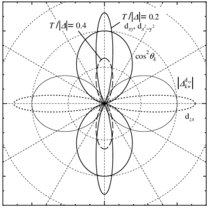
Figure 1: Angular dependence of $-(\Delta_{{{\bm{k}}}+}/T)f^{\prime}(\Delta_{{{\bm{k}}}+})$ on the Fermi surface, where $\varphi_{{{\bm{k}}}}=\pi/4$ for the ${\rm d}_{xy}$ and ${\rm d}_{yz}$ wave states and $\varphi_{{{\bm{k}}}}=0$ for the ${\rm d}_{x^{2}-y^{2}}$ wave state.

3 Numerical Results

In this section, we calculate $\chi_{1}$ that contributes to the temperature-dependent component of the Knight shift. We solve the gap equation numerically [12]. For simplicity, we do not consider mixing different d-wave order parameters.

Figure 2 plots the numerical results. The curves for the ${\rm d}_{xy}$- and ${\rm d}_{x^{2}-y^{2}}$-wave states, which coincide, are upward convex, while those for the ${\rm d}_{yz}$-, ${\rm d}_{zx}$-, ${\rm d}_{3z^{2}-r^{2}}$-, and s-wave states are downward convex. Therefore, the former states are more stable against a magnetic field along the $z$-axis than the latter states are.

Figure 2: Temperature dependences of the intraband components $\chi_{1}$ of the spin susceptibilities for the five d-wave states and the s-wave state. The solid curve is for both ${\rm d}_{xy}$ and ${\rm d}_{x^{2}-y^{2}}$ wave pairing, which coincide. The dot-dashed curve is for the ${\rm d}_{yz}$ and ${\rm d}_{zx}$ wave pairing and the 2 dot-dashed curve is for ${\rm d}_{3z^{2}-y^{2}}$ pairing. The dashed curve plots the results for s-wave pairing. The dotted and thin solid curves present the results for Cases (a) and (c), respectively.

Because of this result, we consider the following conditions [Cases (a) – (c)] for polycrystalline powder samples: (a) the orientations of the powder particles are random, (b) for all powder particles, the ${\rm d}_{xy}$ or ${\rm d}_{x^{2}-y^{2}}$ wave state is realized, and (c) for a portion of the sample, the ${\rm d}_{xy}$ or ${\rm d}_{x^{2}-y^{2}}$ wave state is realized while, for the rest, the superconductivity is destroyed.

For Case (a), the gap function is oriented randomly in each powder particle. This can be mathematically expressed by changing the polar axis randomly for polar coordinates in $\Delta_{{{\bm{k}}}+}^{(\alpha)}$, i.e., by replacing $\Delta_{{{\bm{k}}}+}^{(\alpha)}(\theta_{\hat{{\bm{k}}}},\varphi_{\hat{{\bm{k}}}})$ with $\Delta_{{{\bm{k}}}+}^{(\alpha)}(\theta^{\prime}_{\hat{{\bm{k}}}},\varphi^{\prime}_{\hat{{\bm{k}}}})$, where $(\theta^{\prime}_{\hat{{\bm{k}}}},\varphi^{\prime}_{\hat{{\bm{k}}}})$ are the polar coordinates for the new random polar axis, and the factor $\cos^{2}\theta_{\hat{{\bm{k}}}}$ in $\chi_{1}$ remains unaffected. Since the original polar axis for $(\theta_{\hat{{\bm{k}}}},\varphi_{\hat{{\bm{k}}}})$ is parallel to the uniform magnetic field, the angle between the two polar axes is random. Therefore, the spin susceptibility of the bulk sample is obtained by replacing the factor $\cos^{2}\theta_{\hat{{\bm{k}}}}$ with the angle average on the Fermi surface, which is equal to $1/3$ in the present spherically symmetric system.

Case (b) can occur when the system is affected by the magnetic field so that the spin polarization energy is lowered. This situation can be realized by the following mechanisms: (b-1) when some of the d-wave states are approximately degenerate, the degeneracy is lifted by the magnetic field in each powder particle, and (b-2) the powder particles are freely rotated by the magnetic field. For Case (b), the factor $\cos^{2}{\bar{\theta}}_{{{\bm{k}}}}$ in $\chi_{1}$ is not averaged.

Case (c) can arise in the presence of the impurity pair-breaking effect [24] in addition to the same conditions as Case (b). The anisotropic superconductivity is fragile against nonmagnetic impurities. As an example, we assume that the superconductivity is destroyed for 50% of the powder particles.

The results for Cases (a) to (c) are shown in Fig. 2. The reduction of the spin susceptibility because of the growth of the superconducting gap in the ${\rm d}_{xy}$ and ${\rm d}_{x^{2}-y^{2}}$ wave states is smaller than that in the s-wave state and the other d-wave states. The graph for Case (a) shown in Fig. 2 is the result of $\chi_{1}(T)$ for ${\rm d}_{xy}$, ${\rm d}_{yz}$, ${\rm d}_{zx}$, and ${\rm d}_{x^{2}-y^{2}}$ wave pairing, which coincide. The result for ${\rm d}_{3z^{2}-y^{2}}$ wave pairing is rather different from these.

Next, we compare the theoretical results in Cases (a) – (c) with the experimental data given in Ref. Nis07 by the following procedure: (i) determine $\Delta K^{\rm Pd}(0)=|A_{\rm hf}|\chi_{\rm 1N}^{\rm Pd}$ by comparing the theoretical curve for the s-wave state and the experimental data of ${\rm Li_{2}Pd_{3}B}$, (ii) estimate $\Delta K^{\rm Pt}(0)=|A_{\rm hf}|\chi_{\rm 1N}^{\rm Pt}$ from the value of $\Delta K^{\rm Pd}(0)$, (iii) determine $K^{\rm Pt}(T_{\rm c}^{\rm Pt})$ from the Knight shift data above $T_{\rm c}^{\rm Pt}$ in ${\rm Li_{2}Pt_{3}B}$, and (iv) plot theoretical curves of

$$K^{\rm Pt}(T)=K^{\rm Pt}(T_{\rm c}^{\rm Pt})+\Delta K^{\rm Pt}(0)\frac{\Delta\chi_{1}^{\rm Pt}(T)}{\Delta\chi_{1}^{\rm Pt}(0)}$$

in Cases (a) – (c).

In Step (i), we obtain $K^{\rm Pd}(T_{\rm c}^{\rm Pd})\approx 0.075$% and $K^{\rm Pd}(0)\approx 0.0835$%, which leads to $|\Delta K^{\rm Pd}(0)|\approx 0.0085$%. The values of $K^{\rm Pd}(0)$ and $K^{\rm Pt}(0)$ include the contribution from $\chi_{\rm V}=\chi_{2}+\chi_{3}$. In Step (ii), considering the reduction of the density of states examined by Maruyama and Yanase [23], we assume that $\displaystyle{\chi_{\rm 1N}^{\rm Pt}\sim\chi_{\rm 1N}^{\rm Pd}/2}$, because one of the spin-orbit split Fermi-surfaces disappears. Assuming that $A_{\rm hf}$’s are on the same order in the two compounds, we obtain $\Delta K^{\rm Pt}(0)=0.00425$%. In Step (iii), we obtain $K^{\rm Pt}(T_{\rm c}^{\rm Pt})\approx 0.0725$%, from the Knight shift data above $T_{\rm c}^{\rm Pt}=2.1$ K in ${\rm Li_{2}Pt_{3}B}$.

Figure 3: Comparison between the experimental data and the theoretical curves for Cases (a) – (c). The closed circles, open circles, and open diamonds are the experimental data for ${\rm Li_{2}Pd_{3}B}$ and $H=1.46$ T, ${\rm Li_{2}Pt_{3}B}$ and $H=0.26$ T, and ${\rm Li_{2}Pt_{3}B}$ and $H=0.35$ T, respectively, from Ref. Nis07. The dashed and short dashed curves plot the results of s-wave pairing in ${\rm Li_{2}Pd_{3}B}$ and ${\rm Li_{2}Pt_{3}B}$, respectively. The dotted, solid, and thin sold curves present the results of Cases (a) – (c) for ${\rm Li_{2}Pt_{3}B}$, respectively.

The results of Step (iv) are depicted in Fig. 3. For ${\rm Li_{2}Pt_{3}B}$, it is difficult to reproduce the experimental data if s-wave pairing is assumed, in contrast to ${\rm Li_{2}Pd_{3}B}$, as Nishiyama et al. have pointed out. [3, 4] The theoretical result for Case (b) is in better agreement with the experimental data than that of Case (a). Since the length of the error bar shown in Ref. Nis07 is approximately $\pm 0.003$%, the result for Case (b) sufficiently reproduces the experimental data, within the experimental resolution. The result for Case (c) agrees very well with the experimental data, where it is assumed that the superconductivity is destroyed in half of the powder particles. The Knight shift slightly increases near $T=0$ in the experimental data for ${\rm Li_{2}Pt_{3}B}$, although the increase is smaller than the error bar. For Cases (a) and (c), there are spatial distributions of spin susceptibility, which broaden the NMR spectra. However, the additional peak width would be much smaller than the original peak width because of dipole-dipole interaction, which is discussed in Ref. Nis07.

4 Summary and Conclusions

In noncentrosymmetric superconductors, the temperature-dependent component of the spin susceptibility $\chi_{1}(T)$ is found to exhibit an upward convex curve below ${T_{\rm c}}$ for ${\rm d}_{xy}$- and ${\rm d}_{x^{2}-y^{2}}$-wave pairing, and a downward convex curve for ${\rm d}_{yz}$, ${\rm d}_{zx}$, and ${\rm d}_{3z^{2}-r^{2}}$ wave pairing, when ${{\bm{H}}}\parallel{\hat{{\bm{z}}}}$. Therefore, the ${\rm d}_{xy}$ and ${\rm d}_{x^{2}-y^{2}}$ wave states are most stable in a magnetic field among the d-wave states. To explain the qualitative difference in the temperature dependence of the Knight shift in ${\rm Li_{2}Pd_{3}B}$ and ${\rm Li_{2}Pt_{3}B}$ polycrystalline powder samples, we have assumed three Cases (a) – (c). For Case (b), the observed behaviors of the Knight shifts in ${\rm Li_{2}Pd_{3}B}$ and ${\rm Li_{2}Pt_{3}B}$ are consistently explained within the experimental resolution. For Case (c), the agreement between theory and experiment is excellent. In conclusion, the Knight shift data can be consistently explained if we assume that a full-gap state and a line-node state are realized in ${\rm Li_{2}Pd_{3}B}$ and ${\rm Li_{2}Pt_{3}B}$, respectively.

The present analysis can be extended to other anisotropic pairings and other forms of $\alpha_{{{\bm{k}}}}{{{\bm{g}}}}({{\bm{k}}})$. If the amplitude of the gap function is large only in the region of ${{\bm{k}}}$ where $g_{z}({{\bm{k}}})=\cos{\bar{\theta}}_{{{\bm{k}}}}$ is small, the temperature dependent component of the spin susceptibility $\chi_{1}$ is enhanced, and its temperature dependence curve can be upward convex. In particular, if $\Delta_{{{\bm{k}}}}\approx 0$ for any ${{\bm{k}}}$ such that $g_{z}({{\bm{k}}})=\cos{\bar{\theta}}_{{{\bm{k}}}}\neq 0$, we obtain $\chi_{1{\rm S}}\approx\chi_{1{\rm N}}$. The planar system in which ${{\bm{g}}}({{\bm{k}}})$ is perpendicular to a single constant vector ${{\bm{c}}}$ for all ${{\bm{k}}}$ is an extreme case. In this case, $\chi_{1{\rm S}}=\chi_{1{\rm N}}$ for any pairing anisotropy, when ${{\bm{H}}}\parallel{{\bm{c}}}$. The Rashba spin-orbit interaction ${\hat{{\bm{g}}}}({{\bm{k}}})={\hat{{\bm{k}}}}\times{{\bm{z}}}$ is a typical example [18]. In such systems, if the orientations of the powder particles or the gap functions are modified by a magnetic field, as in Case (b), so that the spin polarization energy is minimized, the difference in the Knight shifts in the superconducting and normal phases can be small.

Acknowledgments

We are very grateful to H. Tou, T. Shishidou, and Y. Yanase for useful discussions. We would also like to thank G.-Q. Zheng for the experimental data.

References

- [1] K. Togano, P. Badica, Y. Nakamori, S. Orimo, H. Takeya, and K. Hirata, Phys. Rev. Lett. 93, 247004 (2004).
- [2] P. Badica, T. Kondo, and K. Togano, J. Phys. Soc. Jpn. 74, 1014 (2005).
- [3] M. Nishiyama, Y. Inada, and G.-Q. Zheng, Phys. Rev. B 71, 220505(R) (2005).
- [4] M. Nishiyama, Y. Inada, and G.-Q. Zheng, Phys. Rev. Lett. 98, 047002 (2007).
- [5] H. Q. Yuan, D. F. Agterberg, N. Hayashi, P. Badica, D. Vandervelde, K. Togano, M. Sigrist, and M. B. Salamon, Phys. Rev. Lett. 97, 017006 (2006).
- [6] H. Takeya, K. Hirata, K. Yamaura, K. Togano, M. El Massalami, R. Rapp, F. A. Chaves, and B. Ouladdiaf, Phys. Rev. B 72, 104506 (2005).
- [7] H. Takeya, M. El Massalami, S. Kasahara, and K. Hirata, Phys. Rev. B 76, 104506 (2007).
- [8] D. C. Peets, G. Eguchi, M. Kriener, S. Harada, Sk. Md. Shamsuzzamen, Y. Inada, G.-Q. Zheng, and Y. Maeno, Phys. Rev. B. 84, 054521 (2011).
- [9] L. P. Gor’kov and E. I. Rashba, Phys. Rev. Lett. 87, 037004 (2001).
- [10] I. A. Sergienko and S. H. Curnoe, Phys. Rev. B 70, 214510 (2004).
- [11] K. V. Samokhin and V. P. Mineev, Phys. Rev. B 77, 104520 (2008).
- [12] H. Shimahara, J. Phys. Soc. Jpn. 82, 024703 (2013).
- [13] P. A. Frigeri, D. F. Agterberg, A. Koga, and M. Sigrist, Phys. Rev. Lett. 92, 097001 (2004).
- [14] T. Shishidou and T. Oguchi, submitted to Phys. Rev. Lett.
- [15] V. M. Edelstein, Zh. Eksp. Teor. Fiz. 95, 2151 (1989) [Sov. Phys. JETP 68, 1244 (1989)].
- [16] V. M. Edelstein, Phys. Rev. Lett. 75, 2004 (1995).
- [17] S. K. Yip, Phys. Rev. B 65, 144508 (2002).
- [18] P. A. Frigeri, D. F. Agterberg, and M. Sigrist, New J. Phys. 6, 115 (2004).
- [19] S. Fujimoto, Phys. Rev. B 72, 024515 (2005).
- [20] S. Fujimoto, J. Phys. Soc. Jpn. 76, 034712 (2007).
- [21] K. V. Samokhin, Phys. Rev. B 76, 094516 (2007).
- [22] S. P. Mukherjee and T. Takimoto, Phys. Rev. B 86, 134526 (2012).
- [23] D. Maruyama and Y. Yanase, J. Phys. Soc. Jpn. 82, 084704 (2013).
- [24] J. P. Carbotte and C. Jiang, Phys. Rev. B 49, 6126 (1994).