Transit timing variations for planets coorbiting
in the horseshoe regime

Abstract

While not detected yet, pairs of exoplanets in the 1:1 mean motion resonance probably exist. Low eccentricity, near-planar orbits, which in the comoving frame follow the horseshoe trajectories, are one of the possible stable configurations. Here we study transit timing variations produced by mutual gravitational interaction of planets in this orbital architecture, with the goal to develop methods that can be used to recognize this case in observational data. In particular, we use a semi-analytic model to derive parametric constraints that should facilitate data analysis. We show that characteristic traits of the transit timing variations can directly constrain the (i) ratio of planetary masses, and (ii) their total mass (divided by that of the central star) as a function of the minimum angular separation as seen from the star. In an ideal case, when transits of both planets are observed and well characterized, the minimum angular separation can also be inferred from the data. As a result, parameters derived from the observed transit timing series alone can directly provide both planetary masses scaled to the central star mass.

1 Introduction

Stable configurations of planets in the 1:1 mean motion resonance (MMR) comprise three different cases: (i) tadpole orbits, which are similar to the motion of Trojan asteroids near Jupiter’s L4 and L5 stationary points, (ii) horseshoe orbits, which are similar to the motion of Saturn’s satellites Janus and Epimetheus, and (iii) binary-planet orbits, in which case the two planets revolve about a common center-of-mass moving about the star on a Keplerian orbit. Numerous studies explored these configurations with different aims and goals. Some mapped stability zones in orbital and parametric spaces. Other studies dealt with formation and/or capture of planets in the 1:1 MMR and their survivability during planetary migration. Still other works explored observational traits such as the radial velocity (RV) signal in stellar spectrum or transit timing variations (TTVs) in the case that one or both planets transit the stellar disk. While we still do not know details of dominant formation and evolutionary processes of planetary systems, as well their variety, a general consensus is that planets in 1:1 MMR should exist. Here we briefly recall several important studies directly related to our work.

Laughlin & Chambers (2002), while studying methods that would reveal a pair of planets in 1:1 MMR from the RV analysis (see also Giuppone et al. 2012), pointed out two possible formation scenarios: (i) planet-planet scattering that would launch one of the planets into a coorbital zone of another planet (including possibly one of the high-eccentricity stable orbital configurations), and (ii) in-situ formation of a smaller planet near the L4 or L5 points of a Jupiter-class planet. These authors also noted that the 1:1 MMR would persist during subsequent migration, since the balance between angular momentum and energy loses prevents an eccentricity increase. This behavior stands in contrast with planets captured in other (higher-order) resonances. Moreover, if significant gas drag is present, the libration amplitude may be damped, thus stabilizing the coorbital configuration.

The suggested scenario of in-situ formation by Laughlin & Chambers (2002) has been modeled by several groups. Beaugé et al. (2007) started with a population of sub-lunar mass planetesimals already assumed to be present in the tadpole region of a giant planet, and studied conditions of coorbiting planet growth. They took into account mutual gravitation interaction of the planetesimals as well as several gas-density models. With this set-up, Beaugé et al. (2007) noted that only $\simeq 0.6$ Earth mass planets grow in their simulations. Beaugé et al. also conducted simulations of planet growth during the migration phase and found essentially the same results. Notably, the Trojan planet orbit has not been destabilized and safely survived migration with a low final eccentricity.

A more detailed study has been presented by Lyra et al. (2009). Using a sophisticated model of gas and solid dynamics in a self-gravitating thin disk, these authors modeled planet formation starting with centimeter-size pebbles. They showed that pressure maxima associated with macroscopic vortexes may collect enough particles to generate instability followed by gravitational collapse. Up to $5-20$ Earth mass planets may form this way in the tadpole region of a Jupiter-mass primary, depending on size distribution of the pebble population.

Another pathway toward the formation of low-eccentricity planets in the 1:1 MMR has been studied by Cresswell & Nelson (2006). These authors analysed the orbital evolution of a compact system of numerous Earth- to super-Earth-mass planets during the dynamical instability phase. If the planetary orbits were initially several Hill radii apart in their simulations, the coorbital configuration emerged as a fairly typical case for some of the surviving planets. A similar set-up, though with different assumptions about the gas-disk density profile, has also been studied by Giuppone et al. (2012), who showed that even similar-mass planets may form in the 1:1 MMR configuration. Additionally, these authors also simulated the coorbital-planet formation and stability during the gas-driven migration. Common to these works was that the 1:1 MMR configuration formed in a sufficiently low-eccentricity state, assisted by efficient gas friction, prior or during the migration stage. If, on the other hand, most of close-in planets formed as a result of tidal evolution from a high-eccentricity state, acquired during the planet-planet scattering (e.g., Beaugé & Nesvorný 2012), and the gas drag was of no help to keep the eccentricities low at any stage of evolution, the fraction of surviving 1:1 MMR configurations may be very small.

Orbital evolution and survival of planets in the 1:1 MMR during migration has also been studied in some detail. For instance, Cresswell & Nelson (2009) considered dynamics of coorbiting planets during and after the gas-disk dispersal and generally found the system to be stable. In some cases, the late migration stage with low-gas friction, or after nebula dispersal, has resulted in an increase of the libration amplitude of the tadpole regime and transition into a horseshoe regime, or even destabilization (see also analysis in Fleming & Hamilton 2000). Rodríguez et al. (2013) included also tidal interaction with the star and found that equal-mass planets may suffer destabilization during their inward migration. Unequal-mass configurations on the other hand that naturally form in the in-situ scenario, may thus be more common.

As far as the detection methods are concerned, the easiest idea would be to seek photometric dips about 1/6 for the hot-Jupiter orbital period away from its transit (as expected for a planet located in the Lagrangian stationary points L4 or L5). However, this approach did not yield so far a positive result (e.g., Rowe et al. 2006, Moldovan et al. 2010). For that reason researchers sought other detection strategies. For instance, Ford & Gaudi (2006) found that a Trojan companion to hot Jupiter might be revealed by detecting an offset between the mid-time of its transit and the zero point of the radial velocity of the star (assuming that barycenter motion is subtracted). This effect would be detectable with available technology for planet companions with at least several Earth masses. While interesting, this method requires a combination of high-quality TTV and RV observations. So far, only upper limits of putative Trojan companions were obtained with this method.

A method based uniquely on analysis of the TTVs of hot Jupiter, if accompanied by a Trojan planet, was discussed by Ford & Holman (2007). While finding the TTV amplitude large enough for even low-mass Trojan companions, Ford & Holman (2007) also pointed out difficulties in interpretation of the data. For instance a Trojan planet on a small-amplitude tadpole orbit would produce nearly sinusoidal TTVs in the orbit of giant planet. Such signal may be produced by a distant moon and/or resonant perturbations due to additional planets in the system. It would take further tests and considerations to prove the signal is indeed due to a Trojan companion.

Haghighipour et al. (2013) presented so far the most detailed study of TTVs produced by a Trojan companion of transiting hot Jupiter. Their main goal was to demonstrate that the expected TTV amplitudes were within the detectable range of Kepler (or even ground-based) observations. With that goal, they first numerically determined the stable region in the orbital phase space. Next, they modeled the TTVs in the hot Jupiter orbit, giving several examples of how the amplitude depends on key parameters of interest (mass of the Trojan companion and eccentricity of its orbit, orbital period of hot Jupiter, etc.). While confirming a confidence of detectability of the produced TTVs, this work did not give any specific hints about inversion problem from TTVs to the system’s parameters neither it discussed uniqueness of the TTV-based determination of Trojan-planet properties.

In this work, we approach the problem with different tools. Namely, we develop a semi-analytic perturbative method suitable for low-eccentricity orbits in the 1:1 MMR. While our method can be applied to the tadpole regime, or even the binary planet configuration, we discuss the case of a coorbital planets on horseshoe orbits. This is because in this case the TTV series have a characteristic shape, which would allow us to most easily identify the orbital configuration (see also Ford & Holman 2007). While the final TTV inversion problem needs to be performed numerically, multi-dimensionality of the parameter space is often a problem. Our formulation allows us to set approximate constraints on several key parameters such as the planetary masses and amplitude of the horseshoe orbit. This information can be used to narrow the volume of parameter space that needs to be searched. Analytic understanding of TTVs is also useful to make sure that a numerical solution is physically meaningful.

2 Model

Following Robutel & Pousse (2013), we use the Poincaré relative variables $({\bf r}_{0},{\bf r}_{1},{\bf r}_{2};{\bf p}_{0},{\bf p}_{1},{\bf p}_{2})$ to describe motion of the star with mass $m_{0}$ and two planets with masses $m_{1}$ and $m_{2}$. It is understood that $(m_{1},m_{2})\ll m_{0}$. The stellar coordinate ${\bf r}_{0}$ is given by its position with respect to the barycenter of the whole system, and the conjugated momentum ${\bf p}_{0}$ is the total (conserved) linear momentum of the system. Conveniently, ${\bf p}_{0}$ is set to be zero in the barycentric inertial system. The coordinates $({\bf r}_{1},{\bf r}_{2})$ of planets are given by their relative position with respect to the star, and the conjugated momenta $({\bf p}_{1},{\bf p}_{2})$ are equal to corresponding linear momenta in the barycentric frame. The advantage of the Poincaré variables stems from their canonicity (e.g., Laskar & Robutel 1995, Goździewski et al. 2008). Their slight caveat is that the coordinates and momenta are given in different reference systems, which can produce non-intuitive effects (see, e.g., Robutel & Pousse 2013). These are, however, of no concern in our work.

Heading toward the perturbation description, the total Hamiltonian ${\cal H}$ of the system is divided into the unperturbed Keplerian part

$${\cal H}_{\rm K}=\sum_{i=1}^{2}\left(\frac{p_{i}^{2}}{2\,\mu_{i}}-G\,\frac{\mu_{i}M_{i}}{r_{i}}\right)\;,$$ (1)

and the perturbation

$${\cal H}_{\rm per}=\frac{{\bf p}_{1}\cdot{\bf p}_{2}}{m_{0}}-G\,\frac{m_{1}m_{2}}{\left|{\bf r}_{1}-{\bf r}_{2}\right|}\;.$$ (2)

Here we denoted $M_{i}=m_{0}+m_{i}$ and the reduced masses $\mu_{i}=m_{0}m_{i}/M_{i}$ for the planets $i=1,2$. The gravitational constant is denoted by $G$.

For sake of simplicity, we restrict the analysis to the planar configuration. The reference plane of the coordinate system is then chosen to coincide with the orbital plane of the two planets around the star. As a result, the planetary orbits are described by only four orbital elements: semimajor axis $a$, eccentricity $e$, longitude of pericenter $\varpi$ and mean longitude in orbit $\lambda$. To preserve canonicity of the orbital parameters, and to deal with orbits of small eccentricity, we adopt Poincaré rectangular variables $(\lambda,\Lambda;x,-\imath\bar{x})$, instead of the simple Keplerian set, to describe orbits of both planets ($\imath=\sqrt{-1}$ and over-bar meaning complex conjugate operation). Here the momentum conjugated to the longitude of orbit $\lambda$ is the Delaunay variable $\Lambda=\mu\,\sqrt{GMa}$. The complex coordinate $x=\sqrt{\Lambda}\,\sqrt{1-\sqrt{1-e^{2}}}\,\exp(\imath\varpi)$ has its counterpart in the momentum $-\imath\bar{x}$, both fully describing eccentricity and pericenter longitude. In a very small eccentricity regime we may also use a non-canonical, but simpler, variable $z=e\,\exp(\imath\varpi)=\sqrt{2/\Lambda}\,x+O(x^{3})$.

Since the difference in mean longitudes of the two planets becomes the natural parameter characterizing coorbital motion, it is useful to replace variables $(\lambda_{1},\Lambda_{1};\lambda_{2},\Lambda_{2})$ by

$$\theta_{1} \!\!\!=\!\!\! \lambda_{1}-\lambda_{2}\;,\quad J_{1}=\frac{1}{2}\left(\Lambda_{1}-\Lambda_{2}\right)\;,$$ (3)

$$\theta_{2} \!\!\!=\!\!\! \lambda_{1}+\lambda_{2}\;,\quad J_{2}=\frac{1}{2}\left(\Lambda_{1}+\Lambda_{2}\right)\;.$$ (4)

The advantage is that $(\theta_{1},J_{1};\theta_{2},J_{2})$ remains a set of canonical variables and $\theta_{1}$, with $J_{1}$, are the primary parameters describing the coorbital motion.

The total Hamiltonian ${\cal H}$, expressed in (1) and (2) as a function of Poincaré relative variables, can be transformed with a lot of algebraic labor into a form depending on modified Poincaré rectangular variables $(\theta_{1},J_{1};\theta_{2},J_{2};x_{1},-\imath\bar{x}_{1};x_{2},-\imath\bar{x}_{2})$ (see, e.g., Laskar & Robutel 1995; Robutel & Pousse 2013). In general, ${\cal H}={\cal H}_{\rm K}+{\cal H}_{\rm per}={\cal H}_{0}+\sum_{k\geq 1}{\cal H}_{k}$, where ${\cal H}_{k}\propto x_{1}^{p_{1}}x_{2}^{p_{2}}\bar{x}_{1}^{\bar{p}_{1}}\bar{x}_{2}^{\bar{p}_{2}}$ with positive exponents such that $p_{1}+p_{2}+\bar{p}_{1}+\bar{p}_{2}=k$. Hence, ${\cal H}_{k}$ are of progressively higher orders in the eccentricities of the two planets. We restrict ourselves to the lowest order.

The elegance of the coorbital motion description for small eccentricities is due to a simple, though rich, form of the fundamental Hamiltonian ${\cal H}_{0}$. While we shall return to the role of ${\cal H}_{1}$ and higher-order terms in Sec. 2.2, we first discuss the ${\cal H}_{0}$ term. Note that ${\cal H}_{0}$ contains both the Keplerian term ${\cal H}_{\rm K}$ and the fundamental part of the planetary interaction in ${\cal H}_{\rm per}$.

2.1 Dynamics corresponding to the ${\cal H}_{0}$ term

We find that

$${\cal H}_{0} = -\,G\,\frac{\mu_{1}M_{1}}{2a_{1}}-G\,\frac{\mu_{2}M_{2}}{2a_{2}}$$

$$+\,Gm_{1}m_{2}\left[\frac{\cos\theta_{1}}{\sqrt{a_{1}a_{2}}}-\frac{1}{\Gamma\left(a_{1},a_{2},\theta_{1}\right)}\right]\;,$$

where the dependence on the orbital semimajor axes $a_{1}$ and $a_{2}$ of the planets only serves to keep this expression short; the Hamiltonian is truly a function of the momenta $(J_{1},J_{2})$ via

$$a_{1} = \frac{\left(J_{1}+J_{2}\right)^{2}}{G\mu_{1}^{2}M_{1}}\;,$$ (6)

$$a_{2} = \frac{\left(J_{1}-J_{2}\right)^{2}}{G\mu_{2}^{2}M_{2}}\;.$$ (7)

Additionally, we have

$$\Gamma\left(a_{1},a_{2},\theta_{1}\right)=\sqrt{a_{1}^{2}+a_{2}^{2}-2a_{1}a_{2}\cos\theta_{1}}\;,$$ (8)

which is not to be developed in Taylor series for description of the coorbital motion at this stage. We also note that a factor $m_{0}/\sqrt{M_{1}M_{2}}$ has been omitted in the first term of the bracket in Eq. (2.1). This is a fairly good approximation for planetary masses much smaller than the stellar mass. We observe that the coordinate $\theta_{2}$ is absent in ${\cal H}_{0}$, implying that the conjugated momentum $J_{2}$ is constant. The $J_{2}$ conservation is just a simpler form of a general angular momentum integral $2J_{2}-|x_{1}|^{2}-|x_{2}|^{2}=C_{1}$ at this level of approximation (eccentricities neglected). The motion is thus reduced to a single degree of freedom problem ${\cal H}_{0}(\theta_{1},J_{1};J_{2})=C_{2}$, where $C_{2}$ is constant. The $C_{2}$ isolines in the $(\theta_{1},J_{1})$ space provide a qualitative information of system’s dynamics.

Further development is driven by observation that in the coorbital regime $a_{1}$ and $a_{2}$ are both very close to some average value $a_{0}$. As discussed by Robutel & Pousse (2013), $a_{0}$ may conveniently replace the constant $J_{2}$ momentum using

$$J_{2}=\frac{1}{2}\left(\mu_{1}\sqrt{GM_{1}}+\mu_{2}\sqrt{GM_{2}}\right)\sqrt{a_{0}}\;,$$ (9)

In the same time, it is advantageous to introduce a small quantity, which will characterize small deviation of $a_{1}$ and $a_{2}$ from $a_{0}$. This is accomplished by replacing $(\theta_{1},J_{1})$ with $(\theta,J)$ using a simple shift in momentum:

$$J_{1}=\frac{1}{2}\left(\mu_{1}\sqrt{GM_{1}}-\mu_{2}\sqrt{GM_{2}}\right)\sqrt{a_{0}}+J\;,$$ (10)

and $\theta_{1}=\theta$. So now ${\cal H}_{0}={\cal H}_{0}(\theta,J;a_{0})$. Finally, it is useful to define a dimensionless and small parameter $u$ instead of $J$ by $J=(\mu_{1}+\mu_{2})\sqrt{Gm_{0}a_{0}}\,u$ even at expense, that $u$ is not canonically conjugated to $\theta$. The dynamical evolution of the system is then described by quasi-Hamiltonian equations

$$\frac{du}{dt}=-\frac{1}{c}\frac{\partial{\cal H}_{0}}{\partial\theta}\;,\quad\frac{d\theta}{dt}=\frac{1}{c}\frac{\partial{\cal H}_{0}}{\partial u}\;,$$ (11)

with $c=(\mu_{1}+\mu_{2})\sqrt{Gm_{0}a_{0}}$. At this moment it is also useful to relate $(\theta,u)$ to the semimajor axes of the two planets via

$$a_{1} = a_{0}\left(1+\frac{\mu_{1}+\mu_{2}}{\mu_{1}}\sqrt{\frac{m_{0}}{M_{1}}}\,u\right)^{2}\;,$$ (12)

$$a_{2} = a_{0}\left(1-\frac{\mu_{1}+\mu_{2}}{\mu_{2}}\sqrt{\frac{m_{0}}{M_{2}}}\,u\right)^{2}\;,$$ (13)

and ${\cal H}_{0}$ still given by Eq. (2.1). These relations permit to compute differentiation with respect to $u$ using the chain rule, such as

$$\frac{\partial}{\partial u}=\frac{\partial a_{1}}{\partial u}\frac{\partial}{\partial a_{1}}+\frac{\partial a_{2}}{\partial u}\frac{\partial}{\partial a_{2}}\;.$$ (14)

Once the solution the planet motion in new variables $u(t)$ and $\theta(t)$ is obtained, we shall also need to know mean longitudes, $\lambda_{1}$ and $\lambda_{2}$, to determine TTVs. To that end we invert Eqs. (3) and (4), obtaining

$$\lambda_{1} = \frac{1}{2}\,\left(\theta_{2}+\theta\right)\;,$$ (15)

$$\lambda_{2} = \frac{1}{2}\,\left(\theta_{2}-\theta\right)\;,$$ (16)

and find $\theta_{2}(t)$ from the integration of

$$\frac{d\theta_{2}}{dt}=\frac{\partial{\cal H}_{0}}{\partial J_{2}}\;.$$ (17)

Differentiation with respect to $J_{2}$ is obtained by the chain rule with Eqs. (6) and (7).

It is also useful to recall that $\theta$ evolves more slowly than $\theta_{2}$, since to the lowest order in $u$: $d\theta_{2}/dt\propto u^{0}$, while $d\theta/dt\propto u^{1}$. In fact, the unperturbed solution reads $\theta_{2}\simeq 2\,n_{0}(t-t_{0})$, with

$$n_{0}=\sqrt{\frac{Gm_{0}}{a_{0}^{3}}}\;,$$ (18)

implying $\lambda_{1}=\lambda_{2}\simeq n_{0}\left(t-t_{0}\right)$ to the lowest order.

Note that so far we considered the exact solution of ${\cal H}_{0}$, without referring to approximations given by its expansion in small quantities: $u$, and $m_{1}/m_{0}$ and $m_{2}/m_{0}$. The reason for this was twofold. First, we found such series may converge slowly and truncations could degrade accuracy of the solution. Second, although we find it useful to discuss some aspects of such development in the small parameters below, we note that the system is not integrable analytically at any meaningful approximation. This implies that semi-numerical approach is anyway inevitable. Considering the complete system, as opposed to approximations given by truncation of series in the above mentioned small parameters, does not extent the CPU requirements importantly. In fact, Eqs. (11) and (17) are easily integrated by numerical methods (in our examples below we used simple Burlish-Stoer integrator leaving implementation of more efficient symplectic methods for future work).

Figure 1: Example of two trajectories in the $(u,\theta)$ phase space of Hamiltonian ${\cal H}_{0}$; for sake of illustration we used $m_{0}=1$ M_⊙, $m_{1}/m_{0}=10^{-3}$ and $m_{2}/m_{0}=2\times 10^{-5}$. The trajectory in a horseshoe regime, labeled H, is characterized by: (i) minimum and maximum value of $|u|$ parameter (denoted here $u_{1}$ and $u_{2}$), and (ii) minimum angular separation $\theta_{\rm min}$ of the coorbiting planets. The trajectory labeled T shows an example of a tadpole orbit, librating about the Lagrangian stationary point L4 for comparison.

While numerical approach provides an exact solution, it is still useful to discuss some qualitative aspects by using the approximated forms of ${\cal H}_{0}$. The smallness of $u$ permits denominator factors such as $1/\Gamma$ in Eq. (2.1) be developed in power series of which we preserve terms up to the second order (see also Robutel & Pousse 2013):

$${\cal H}_{0}\left(\theta,u;a_{0}\right)=\frac{G}{a_{0}}\left(A_{0}+A_{1}\,u+A_{2}\,u^{2}\right)\;.$$ (19)

The $A$-coefficients read

$$A_{0} \!\!\!=\!\!\! \frac{\sigma}{2}\left(2-\gamma^{2}-\frac{2}{\gamma}\right)\;,$$ (20)

$$A_{1} \!\!\!=\!\!\! -\frac{\sigma_{+}\sigma_{-}}{2}\left(1-\gamma\right)^{2}\left(1+\frac{2}{\gamma}\right)\;,$$ (21)

$$A_{2} \!\!\!=\!\!\! -\frac{3}{2}\frac{m_{0}\sigma_{+}^{3}}{\sigma}+$$

$$\frac{\sigma_{+}^{2}}{\sigma}\left[\left(\sigma_{+}^{2}-3\sigma\right)\left(4-\frac{\gamma^{2}}{2}-\frac{1}{\gamma}\right)+\frac{2\sigma_{+}^{2}}{\gamma^{3}}\right]\;,$$

with the mass-dependent parameters $\sigma_{\pm}=m_{1}\pm m_{2}$ and $\sigma=m_{1}m_{2}$, and $\gamma=\sqrt{2-2\cos\theta}$. Terms to the second power of planetary masses have been retained in Eq. (19). In fact, the simplest form is obtained by dropping the linear term in $u$, and approximating $A_{2}$ by the first factor only. This results in

$${\cal H}_{0}=-\frac{3}{2}\frac{G}{a_{0}}\frac{m_{0}\sigma_{+}^{3}}{\sigma}u^{2}+\frac{G\sigma}{a_{0}}\left(\cos\theta-\frac{1}{\gamma}\right)\;,$$ (23)

introduced already by Yoder et al. (1983) (see also Sicardy & Dubois 2003). Hamiltonian (23) corresponds to a motion of a particle in the potential well

$$U\left(\theta\right)=\cos\theta-\frac{1}{\gamma(\theta)}\;.$$ (24)

As discussed by Robutel & Pousse (2013), in both approximations (19) and (23) the exact character of motion is not represented near $\Gamma\simeq 0$, corresponding to a collision configuration, but this is not of great importance for us.

Unfortunately, the Hamiltonian (23) is not integrable analytically. Still, the energy conservation ${\cal H}_{0}=C_{2}$ provides a qualitative insight into trajectories in $(u,\theta)$ space and also allows us to quantitatively estimate some important parameters. Figure 1 shows examples of two trajectories in phase space of $(u,\theta)$, one corresponding to a horseshoe solution (H) and one corresponding to a tadpole solution (T) librating about the L4 Lagrangian stationary solution. Here, we set $m_{0}$ equal to solar mass, $m_{1}/m_{0}=10^{-3}$ and $m_{2}/m_{0}=2\times 10^{-5}$. Since we are primarily focusing on the horseshoe coorbital regime, we determine relations between parameters characterizing the H-trajectory in Fig. 1. These are the: (i) minimum $u_{1}$ and maximum $u_{2}$ amplitudes of $|u|$ along the trajectory, (ii) minimum separation angle $\theta_{\rm min}$, and (iii) half-period $T$ of motion along the trajectory in the $(u,\theta)$ space. One easily finds that $u_{1}$ corresponds to planetary opposition $\theta=\pm\pi$, and $u_{2}$ corresponds to longitude of the Lagrangian stationary solutions $\theta=\pm\pi/3$. As a result

$$u_{2}^{2}-u_{1}^{2}=\frac{2}{3}\frac{\sigma^{2}}{m_{0}\sigma_{+}^{3}}\;.$$ (25)

The symmetry of ${\cal H}_{0}$ in $u$ implies that $\theta_{\rm min}$ corresponds to $u=0$, and thus

$$u_{1}^{2}=\frac{1}{3}\frac{\sigma^{2}}{m_{0}\sigma_{+}^{3}}\left(2\,\Sigma_{\rm min}+\sqrt{\frac{2}{\Sigma_{\rm min}}}-5\right)\;,$$ (26)

where we denoted $\Sigma_{\rm min}=1-\cos\theta_{\rm min}$. The inverse relation requires solution of a cubic equation, conveniently given in the standard form. By using the trigonometric formulas one has

$$\Sigma_{\rm min}=\frac{4\,K}{3}\cos^{2}\left[\frac{1}{3}\,{\rm acos}\left(\sqrt{\frac{27}{8\,K^{3}}}\right)-\frac{2\pi}{3}\right]\;,$$ (27)

with

$$K=\frac{3}{2}\frac{m_{0}\sigma_{+}^{3}}{\sigma^{2}}\,u_{1}^{2}+\frac{5}{2}\;.$$ (28)

The critical trajectory, representing transition between the horseshoe and tadpole orbits, has $u_{1}=0$, thus $K=5/2$. Equation (27) then provides a formula for a maximum value of $\theta_{\rm min}$ separation in the horseshoe regime, roughly $23.9^{\circ}$. The minimum value of $\theta_{\rm min}$ is approximately set by Lagrangian $L_{1}$ and $L_{2}$ stationary points of the ${\cal H}_{0}$ Hamiltonian. Robutel & Pousse (2013) show that this minimum separation value is $\simeq\text@frac{4}{5}(\sigma_{+}/6m_{0})^{1/3}$. Depending on planetary masses defining $\sigma_{+}/m_{0}$ this may be few degrees.

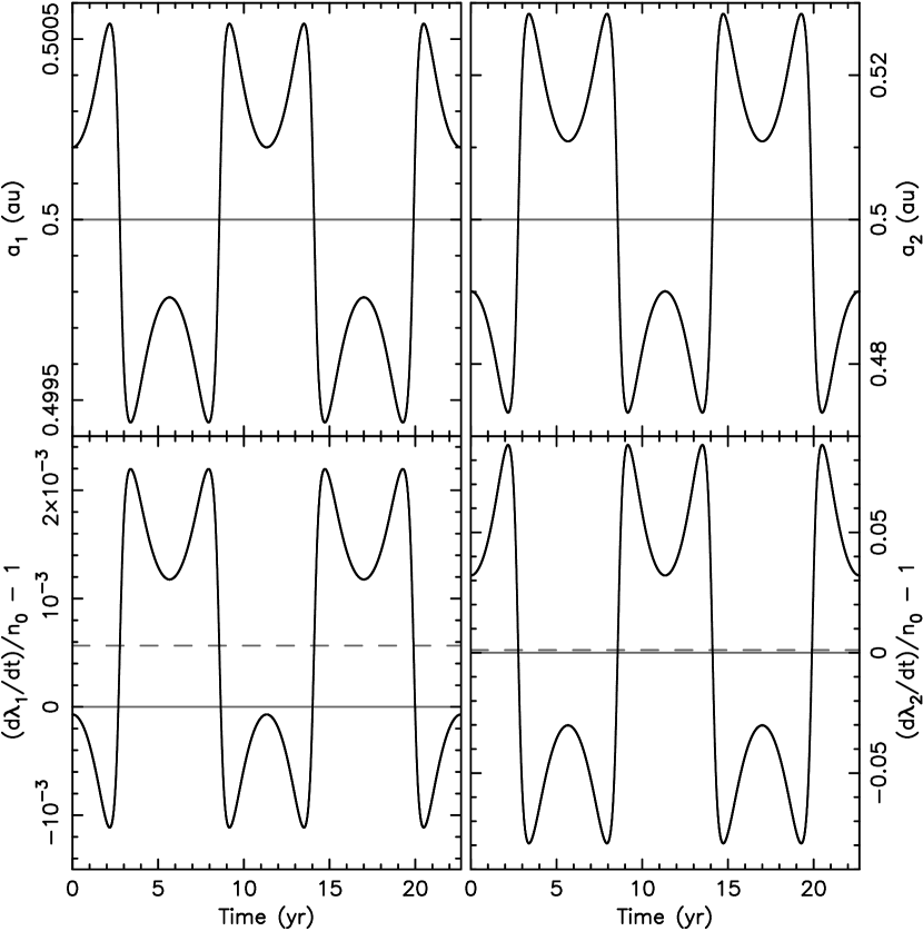
Figure 2: Top: Semimajor axis $a_{1}$ of the heavier planet (left) and the lighter planet $a_{2}$ (right) as a function of time for the horseshoe trajectory in Fig. 1. Their mean value $a_{0}=0.5$ au, for definiteness. The timespan covers two cycles of the circulation along the trajectory. The lighter planet experiences larger perturbations and thus larger-amplitude variations of the semimajor axis. Bottom: Normalized rates of change of the longitude in orbit $(d\lambda_{1}/dt)/n_{0}-1$ of the heavier planet (left) and the lighter planet $(d\lambda_{2}/dt)/n_{0}-1$ (right). The dashed horizontal lines are numerically computed mean values. They are offset from zero for reasons discussed in the main text.

Finally, the relation between $T$ and $\theta_{\rm min}$ is obtained from the energy conservation:

$$\sqrt{\frac{3}{2}\frac{\sigma_{+}}{m_{0}}}\,n_{0}T=\int_{\theta_{\rm min}}^{\pi}\frac{d\theta}{\sqrt{U(\theta)-c_{2}}}\;,$$ (29)

where $c_{2}=C_{2}(a_{0}/G\sigma)=U(\theta_{\rm min})=1-K$, with $K$ given above. Obviously, $a_{0}$ is now needed to gauge $n_{0}$, while $c_{2}$ may be obtained as a function of either of the parameters $u_{1}$, $u_{2}$ or $\theta_{\rm min}$( see Eq. (28)). If one wants the right hand side in (29) be solely a function of $\theta_{\rm min}$, we have

$$c_{2}=1-\left(\Sigma_{\rm min}+\frac{1}{\sqrt{2\,\Sigma_{\rm min}}}\right)\;.$$ (30)

Figure 2 shows time evolution of the semimajor axes $a_{1}$ and $a_{2}$, and mean orbital longitude rates for the exemplary system shown in Fig. 1 ($m_{0}=1$ M_⊙, $m_{1}/m_{0}=10^{-3}$, $m_{2}/m_{0}=2\times 10^{-5}$, and $a_{0}=0.5$ au). In this case we focus on the horseshoe orbit denoted H on Fig. 1. The longitude rates, computed from their definition (15) and (16) and using Eqs. (11) and (17), are represented in a normalized way by $(d\lambda_{1}/dt)/n_{0}-1$ and $(d\lambda_{2}/dt)/n_{0}-1$. As the trajectory moves along the oval-shaped curve in the phase space, the orbits periodically switch their positions with respect to the star causing their semimajor axis to jump around the $a_{0}$ value. Each orbit stays at higher/lower-$a$ regime for time $T$, which is approximately $\propto\sqrt{m_{0}/\sigma_{+}}/3$ longer than its orbital period. The switch in semimajor axes is reflected in the corresponding variations in longitude rate. Note that the average $\lambda$-rates for both orbits are not equal to $n_{0}$ from (18), producing an offset shown by the difference of the dashed line and zero at the bottom panels of Fig. 2. This is because of the planetary masses also contributing to their mean motion about the star, while the definition of $n_{0}$ as a nominal, reference fast frequency did not take this into account. In fact, we find that the longitude rate normalized by $n_{0}$ and averaged over the coorbital cycle $2\,T$ is approximately $1+(m_{i}/2m_{0})+6\,(\sigma_{+}/m_{i})^{2}u_{\star}^{2}+\ldots$ for each of the orbits $(i=1,2)$, with $u_{\star}$ being a characteristic value of the $u$-parameter over one of the half-cycles (e.g., one could approximate $u_{\star}\simeq(u_{1}+u_{2})/2$). When the planetary masses are unequal, as in our example, the more massive planet has the mean longitude rate primarily modified by its own mass. In our case $(d\lambda_{1}/dt)/n_{0}-1\simeq m_{1}/(2m_{0})$. The lighter planet’s longitude rate is dominated by the second term, i.e., in our case $(d\lambda_{2}/dt)/n_{0}-1\simeq 6\,(\sigma_{+}/m_{2})^{2}u_{\star}^{2}$.

Even more important for the TTV analysis is to consider how much the mean rates in longitude change during the coorbital cycle. We find that the change in longitude rates during the low/high-$a$ states for each of the planets is approximated by $\simeq\pm 6\,n_{0}\,(\sigma_{+}/m_{i})\,u_{\star}$ $(i=1,2)$. If large enough, this value may build over a timescale $T$ to produce large variations in the mean longitude of planets, and thus result in large TTVs. We will discuss this in Sec. 3.

2.2 Eccentricity terms

So far, we approximated the interaction Hamiltonian ${\cal H}$ with the leading part ${\cal H}_{0}$ from Eq. (2.1) that is independent of eccentricities $e_{1}$ and $e_{2}$. In order to extend our analysis to the regime of small-$e$ values, we include the lowest-order interaction contributions. Neglecting the second-order eccentricity terms, we have ($z=e\,\exp(\imath\varpi)$)

$$\frac{dz}{dt}=-\frac{2\imath}{\Lambda}\,\frac{\partial{\cal H}}{\partial\bar{z}}\;,$$ (31)

where we insert ${\cal H}={\cal H}_{1}$ and secular part from ${\cal H}={\cal H}_{2}$, the first- and second-order terms in eccentricity development of ${\cal H}$. When $\delta z(t)=z(t)-z(0)$ is known for both orbits from solution of (31), we can compute their effect on TTVs by defining (e.g., Nesvorný & Vokrouhlický 2014)

$$\delta\lambda^{\rm eff}=\imath\left(\delta z\,e^{-\imath\lambda_{0}}-\delta\bar{z}\,e^{\imath\lambda_{0}}\right)\;.$$ (32)

Here $\lambda_{0}$ is the unperturbed longitude in orbit for which we substitute the zero-order solution $\lambda_{0}=n_{0}(t-t_{0})$ plus a phase, individual to each of the two planets. This is an effective change in orbital longitude given here to the first order in eccentricity (see Nesvorný 2009 for higher order terms), which together with the direct effect in $\lambda$ contributes to TTVs. It is not known a priori which of these contributions should be more important. For instance, in the case of closely packed (but not coorbiting) orbits studied by Nesvorný & Vokrouhlický (2014), the eccentricity term (32) was generally larger than the direct perturbation in $\lambda$ over a short-term timescale.

We should also note that the ${\cal H}_{1}$ and ${\cal H}_{2}$ Hamiltonians would also contribute to variations of the $(u,\theta,\theta_{2})$ variables. Perhaps the most interesting effect should be a slight modification of the planetary mean motion through the change in $\theta_{2}(t)$. However, since it is not our intention to develop a complete perturbation theory for coorbital motion here, we neglect these terms focusing on the lowest-order eccentricity effects. We verified that a slight change in initial conditions, specifically the $u$ parameter value, would equivalently represent the eccentricity modification of the $\theta_{2}(t)$ angle.

2.2.1 First-order terms

We start with the first-order eccentricity terms in ${\cal H}_{1}$. While apparently of a larger magnitude in ${\cal H}$ than ${\cal H}_{2}$, they are short-periodic and this diminishes their importance. An easy algebra shows that the perturbation equations read (recall that the overbar means complex conjugation)

$$\frac{dz_{1}}{dt} \!\!=\!\! -n_{0}\,\frac{m_{2}}{m_{0}}\,\Phi\left(\theta\right)\,e^{\imath\theta_{2}/2}\;,$$ (33)

$$\frac{dz_{2}}{dt} \!\!=\!\! \phantom{-}n_{0}\,\frac{m_{1}}{m_{0}}\,{\bar{\Phi}}\left(\theta\right)\,e^{\imath\theta_{2}/2}\;,$$ (34)

with

$$\Phi\left(\theta\right)=\imath\,e^{3\imath\theta/2}+\frac{\sin\frac{1}{2}\theta}{\gamma^{3}}\left(3+e^{\imath\theta}\right)\;.$$ (35)

We neglected terms of the order $u$ and higher in the right hand sides of (33) and (34), and used $\gamma=\gamma(\theta)=\sqrt{2-2\cos\theta}$. Since $\theta_{2}/2\simeq n_{0}(t-t_{0})$, the power-spectrum of the right hand sides in (33) and (34) is indeed dominated by the high (orbital) frequency $n_{0}$, modulated by slower terms from $\Phi$ dependence on $\theta$.

2.2.2 Second-order terms

The second-order eccentricity terms in ${\cal H}_{2}$ are important, because they are the first in the higher-order ${\cal H}$ expansion part to depend on low-frequencies only. Restricting to this part of ${\cal H}_{2}$, thus dropping the high-frequency component in ${\cal H}_{2}$, we obtain (see Robutel & Pousse 2013)

$$\frac{dz_{1}}{dt} \!\!=\!\! -2\imath\,n_{0}\,\frac{m_{2}}{m_{0}}\left(A\,z_{1}+B\,z_{2}\right)\;,$$ (36)

$$\frac{dz_{2}}{dt} \!\!=\!\! -2\imath\,n_{0}\,\frac{m_{1}}{m_{0}}\left({\bar{B}}\,z_{1}+A\,z_{2}\right)\;,$$ (37)

with

$$A \!\!\!=\!\!\! \frac{1}{8\gamma^{5}}\left(5\cos 2\theta-13\right)-\frac{\cos\theta}{2}\left(1-\frac{1}{\gamma^{5}}\right)\;,$$

$$B \!\!\!=\!\!\! \frac{1}{2}\left(1-\frac{2}{\gamma^{5}}\right)e^{2\imath\theta}+$$

$$\frac{1}{8\gamma^{5}}\left[\imath\sin\theta\left(9-e^{2\imath\theta}\right)+8e^{\imath\theta}\right]\;.$$

We again neglected terms proportional to $u$ and its powers in expressions for $A$ and $B$ for simplicity. While the right hand sides of Eqs. (36) and (37) are of the first order in eccentricities $e_{1}$ and $e_{2}$, they do not contain high-frequency terms and thus the corresponding perturbations may accumulate over time to large values. Indeed, these are the secular perturbations dominating the eccentricity changes.

The equations (33) – (37) do not possess analytical solutions. Therefore, we numerically integrated them together with those for $u$, $\theta$ and $\theta_{2}$, to determine $z_{1}(t)$ and $z_{2}(t)$.

3 An exemplary case

We now give an example of a coorbital system about a solar mass star and compute TTVs by two methods: direct numerical integration of the system in Poincaré relative variables and using the theory presented in Sec. 2.

We used the same planetary configuration whose short-term dynamics was presented in Figs. 1 and 2. In particular, $m_{0}=1$ M_⊙ star with a Jupiter-mass planet $m_{1}=10^{-3}$ M_⊙ coorbiting with a sub-Neptune mass planet $m_{2}=2\times 10^{-5}$ M_⊙. The mean distance from the star was set to be $a_{0}=0.5$ au. The initial orbits were given small eccentricities of $e_{1}=e_{2}=0.01$, and colinear pericenter longitudes $\varpi_{1}=\varpi_{2}=0^{\circ}$. The initial longitude in orbit of both planets were $\lambda_{1}=180^{\circ}$ and $\lambda_{2}=0^{\circ}$, such that at time zero they were at opposition.

Starting with these initial data, we first numerically integrated the motion using Poincaré relative coordinates $({\bf r}_{1},{\bf r}_{2};{\bf p}_{1},{\bf p}_{2})$ introduced in Sec. 1. The equations of motion were obtained from the Hamiltonian ${\cal H}={\cal H}_{\rm K}+{\cal H}_{\rm per}$, with the two parts given by Eqs. (1) and (2). For our simple test we used a general purpose Burlish-Stoer integrator with a tight accuracy control. The integration timespan was $\simeq 22.7$ yr covering two cycles of the coorbital motion (see Fig. 2). For sake of definiteness, we assumed an observer along the x-axis of the coordinate system and we numerically recorded times of transit of the two planets. The transit timing variations were obtained by removing linear ephemeris from transits.

Next, we assumed the system is described by a set of parameters $(u,\theta,\theta_{2};z_{1},z_{2})$ introduced and discussed in Sec. 2, and numerically integrated their dynamical equations (11), (17), and (33-39). For each of the planets we then computed TTVs from (e.g., Nesvorný & Morbidelli 2008, Nesvorný & Vokrouhlický 2014)

$$-n_{\star}\,\delta t=\delta\lambda+\delta\lambda^{\rm eff}\;,$$ (40)

where $n_{\star}$ is the effective mean motion of the unperturbed motion. We use the mean values of the longitude in orbit rate discussed in Sec. 2.1, for instance $n_{\star}=n_{0}\,(1+m_{1}/2m_{0})$ for the Jupiter-mass planet. Having $\theta(t)$ and $\theta_{2}(t)$ integrated, we recover the time-dependence of the longitudes $\lambda_{1}(t)$ and $\lambda_{2}(t)$ from (15) and (16). From these numerically-determined functions we subtracted the average mean motion trend $n_{\star}\,(t-t_{0})$ and obtained variation $\delta\lambda$ of both planets as needed for the computation of TTVs (Eq. 40). The effective eccentricity terms $\delta\lambda^{\rm eff}$ were computed from their definition in Eq. (32).

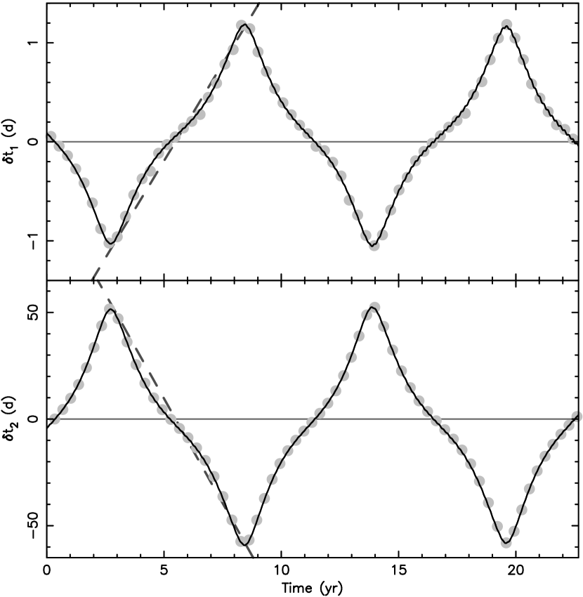
Figure 3: Transit timing variations (TTVs) of the heavier planet $\delta t_{1}$ (top) and the lighter planet $\delta t_{2}$ (bottom). Planetary masses and mean semimajor axis value as in Figs. 1 and 2. The gray symbols are the TTVs obtained from direct numerical integration in Poincaré relative variables (Eqs. 1 and 2). The solid line is from the semi-analytic theory given by Eq. (40). The dashed and sloped lines in both panels are from our expected amplitude of change in longitude rate during the switches between legs in the coorbital cycle; the slope estimate is $\simeq 3\,(\sigma_{+}/m_{i})u_{\star}$, with $u_{\star}\simeq 3.55\times 10^{-4}$ and planets $i=1$ (top) and $i=2$ (bottom). See the main text for more details.

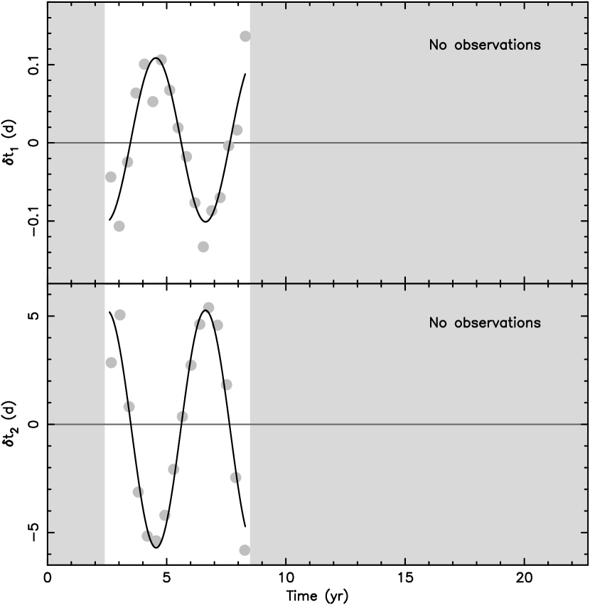
Figure 4: Transit timing variations (TTVs) of the heavier planet $\delta t_{1}$ (top) and the lighter planet $\delta t_{2}$ (bottom) from Fig. 3 if the dataset is limited to observations between 2.6 yr and 8.3 yr. In this case, the analysis would reveal misleading signal with quasi-periodicity of $\simeq 4.2$ yr and much smaller amplitude (solid lines).

Figure 3 shows a comparison between the synthetic TTVs from direct numerical integration (gray symbols) compared to the $\delta t$ function from Eq. (40) (black line). For sake of the example we assumed an ideal situation with both planets transiting. As mentioned in Sec. 2.2, we used a small change in the initial conditions of the secular theory, namely rescaled the $u$ parameter by fractionally $\propto e^{2}$ value, to represent the ${\cal H}_{2}$ effect on the mean motion of planets. With that adjustment, the match between the synthetic TTV series and the modeled function $\delta t$ is excellent. We also note that the contribution of the second term in the right-hand side of (40) is negligible and basically all effect seen on the scale of Fig. 3 is due to the first term (i.e., direct perturbation in orbital longitude). The dashed sloped lines on both panels of Fig. 3 show the effect of a change in mean motion of the planets, as estimated from the simple Hamiltonian (23). In particular their slopes are: (i) $3\,(\sigma_{+}/m_{1})\,u_{\star}$ at the top panel, and (ii) $-3\,(\sigma_{+}/m_{2})\,u_{\star}$ at the bottom panel ($u_{\star}\simeq 3.55\times 10^{-4}$). The match to the mean behavior of the TTVs is good, since in the simplest approximation the planets motion may be understood as a periodic switch between two nearly circular orbits. Since the period $T$ is about 15 times longer than the orbital period of the planets in our case, the effect may accumulate into a large amplitude TTV series.

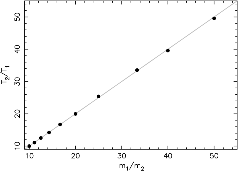
Figure 5: Ratio $T_{2}/T_{1}$ of the maximum amplitude of the TTV series for the less massive planet ($T_{2}$) vs those of the more massive planet ($T_{1}$) placed onto a horseshoe orbit in the 1:1 MMR as determined from the full-fledged numerical integration (ordinate). The abscissa is the planetary mass ratio $m_{1}/m_{2}$. The gray line if the direct proportionality rule obtained from the simplified analytical theory (Sec. 2.1). Details of the set-up are described in the main text.

It is interesting to point out that recognizing the planet’s configuration requires observations covering at least the fundamental period $T$ of the coorbital motion. For instance, if the observations would have covered a shorter interval, say between 2.6 yr and 8.3 yr in Fig. 3, one may not recognize the coorbital signature in the TTVs. Figure 4 shows how the data would have looked in this case. TTV series of both planets would look quasi-periodic with a period $\sim T/2\simeq 4.2$ yr, reflecting behavior of the planets’ mean motion variation over one quarter of the coorbital cycle (i.e., when $\theta$ leaps from $\theta_{\rm min}$ to $360^{\circ}-\theta_{\rm min}$, Fig. 1). Equation (29) indicates that $T\propto a_{0}^{3/2}\,(m_{0}/\sigma_{+})^{1/2}$, making thus the necessary observational timescale (i) shorter for closer-in planets, and (ii) longer for less massive planets. So for instance $\simeq 12$ y periodicity of the TTV series shown in Fig. 3 would also hold for about $8$ Earth mass coorbiting planets at about $0.15$ au distance (i.e., $\simeq 20$ d revolution period) from a solar mass star. These are very typical systems observed by the Kepler satellite.

Consider now an ideal situation when both planets are transiting and a long enough series of TTVs are recorded for both of them (e.g., Fig. 3). Analysis based on approximate Hamiltonian (23) then suggests (Sec. 2.1) that the ratio of maximum amplitudes of the TTV series, to be denoted $T_{1}$ for the more massive planet and $T_{2}$ for the less massive planet, is equal to the ratio of their masses: $T_{2}/T_{1}=m_{1}/m_{2}$. Since $T_{2}/T_{1}$ can be measured from the observations, the mass ratio of the coorbital planets is readily constrained. To verify validity of this conclusion, we numerically integrated a complete Hamiltonian in Poincaré rectangular coordinates with a solar mass star having two coorbital planets with masses $m_{1}=10^{-3}$ M_⊙ and $m_{2}$ ranging values $2\times 10^{-5}$ M_⊙ to $10^{-4}$ M_⊙. We used $a_{0}=0.5$ au and set the planets initially at opposition, i.e. giving them $\lambda_{1}=180^{\circ}$ and $\lambda_{2}=0^{\circ}$. The initial eccentricity values were assumed small, $e_{1}=e_{2}=0.001$, and pericenter longitudes $\varpi_{1}=\varpi_{2}=0^{\circ}$. For each of the mass configurations considered, we followed the system for 1000 yr and derived the synthetic TTV series as shown by symbols in Fig. 3. We then fitted the maximum amplitudes $T_{1}$ and $T_{2}$. Their ratio is shown by black circles in Fig. 5, while the gray line is the expected direct proportionality relation mentioned above. We note the linear trend is a very good approximation.

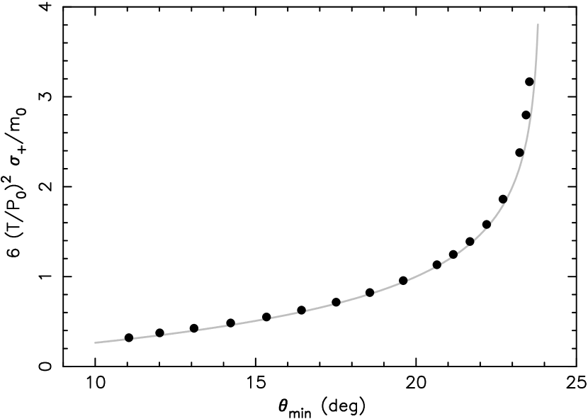
Figure 6: Correlation between the $6\,(T/P_{0})^{2}\,(\sigma_{+}/m_{0})$ parameter (ordinate) and the minimum angular separation $\theta_{\rm min}$ of the coorbiting planets (abscissa). Here $P_{0}$ is the mean orbital period of the planets, $T$ is the half period of the coorbiting cycle, $\sigma_{+}=m_{1}+m_{2}$ is the total mass of the planets and $m_{0}$ is the stellar mass. The black symbols are from direct numerical integration. The gray line is the ${\cal J}(\theta_{\rm min})$ function from Eq. (41), suggested from a simple analytic theory. Beyond $\theta_{\rm min}\simeq 25^{\circ}$ the orbital configuration transits to the tadpole regime.

Another useful parametric constraint is hinted by Eq. (29), again obtained from the simplified Hamiltonian form (23). Denoting for short

$${\cal J}\left(\theta_{\rm min}\right)=\int_{\theta_{\rm min}}^{\pi}\frac{d\theta}{\sqrt{U(\theta)-c_{2}}}\;,$$ (41)

solely a function of the minimum angular separation $\theta_{\rm min}$ of the planets, we have

$$6\,\left(\frac{T}{P_{0}}\right)^{2}\frac{\sigma_{+}}{m_{0}}=\frac{1}{\pi^{2}}\,{\cal J}^{2}\left(\theta_{\rm min}\right)\;.$$ (42)

Here $P_{0}=2\pi/n_{0}$ is a good proxy for the mean orbital period of the planets, $T$ is the half period of the coorbiting cycle (i.e., time between minima and maxima of the TTVs, Fig. 3), and $\sigma_{+}=m_{1}+m_{2}$ as above. Since $T/P_{0}$ can be directly constrained from the observations, Eq. (42) provides a link between the mass factor $\sigma_{+}/m_{0}$ and $\theta_{\rm min}$. We tested the validity of Eq. (42) by directly by integrating the planetary system in Poincaré rectangular coordinates. The model parameters were mostly the same as above, except for: (i) fixing now the planetary masses $m_{1}=10^{-3}$ M_⊙ and $m_{2}=2\times 10^{-5}$ M_⊙, and (ii) starting the two planets at a nominal closest approach, $\lambda_{1}=\theta_{\rm min}$, $\lambda_{2}=0^{\circ}$ and $a_{1}=a_{2}=a_{0}=0.5$ au. Both were given small initial eccentricity $e_{1}=e_{2}=0.001$, and the system was propagated for 1000 yr with the Burlish-Stoer integrator. We recorded series of planetary transits and constructed a synthetic TTVs, similar to ones shown in Fig. 3. The code also provided numerical mean values of the planetary orbital periods, used to compute $P_{0}$, half-period $T$ of the TTV series, and the mean value of the minimum planetary separation. This last parameter was obviously very close to the given initial distance $\theta_{\rm min}$, but typically differed from it by few tenths of a degree because of the effect of planetary eccentricities. With those parameters determined for the direct numerical model, we have all data needed to test the validity of Eq. (42). The results are shown by black circles in Fig. 6. The gray line is the ${\cal J}(\theta_{\rm min})$ integral from Eq. (41), computed by a Romberg’s scheme with controlled accuracy. Note that this integration needs a simple parameter transformation to remove the integrand singularity at $\theta=\theta_{\rm min}$ limit. We note a very good correspondence of the numerical results with the expected trend from the analytic theory.

Figure 7: The observationally available ratio $T/P_{0}$, $T$ is half-period of the TTV series and $P_{0}$ orbital period, on the ordinate vs the minimum separation angle $\theta_{\rm min}$ of the planets during the coorbital cycle. The solid lines, evaluated using Eq. (42), are given for five different values of the mass ratio $m_{0}/\sigma_{+}$ (labels). The gray line at $\theta_{\rm min}=23.9^{\circ}$ indicates the maximum theoretical value, while the true stability limit of $\theta_{\rm min}$ is lower as discussed in the text. The dashed gray lines a and b just set two examples of the $T/P_{0}$ values (see discussion in the text).

Once we verified the validity of Eq. (42), we can use it as shown in Fig. 7. Here the abscissa is the minimum planet separation $\theta_{\rm min}$, while the ordinate is now the ratio $T/P_{0}$ given for a set of different $m_{0}/\sigma_{+}$ values (solid lines). The $T/P_{0}$ factor may be directly constraint from the observations and Fig. 7 hints that this information may be immediately used to roughly delimit the $m_{0}/\sigma_{+}$ factor. This is because $\theta_{\rm min}$ can span only limited range of value for the horseshoe orbits: (i) $\theta_{\rm min}$ cannot approach too closely to the theoretical limit $\simeq 23.9^{\circ}$ derived in Sec. 2.1, especially of $e_{1}$ and $e_{2}$ are non-zero, otherwise instability near the Lagrangian point L3 would onset, and (ii) $\theta_{\rm min}$ cannot be too small, otherwise instability near the Lagrangian points L1 and L2 would onset. While not performing a complete study here, assume for sake of an example that $\theta_{\rm min}$ could be in the interval $\simeq 10^{\circ}$ to $\simeq 22^{\circ}$. Then if $T/P_{0}=10$ is obtained from the observations (as shown by the dashed gray line a in Fig. 7), the $m_{0}/\sigma_{+}$ ratio cannot be much larger than $\sim 2000$. On the other hand, in $T/P_{0}=30$ is obtained from the observations (as shown by the dashed gray line b in Fig. 7), the $m_{0}/\sigma_{+}$ ratio cannot be much smaller than $\sim 3000$. Hence the observations may directly hint the nature of planets in the coorbital motion.

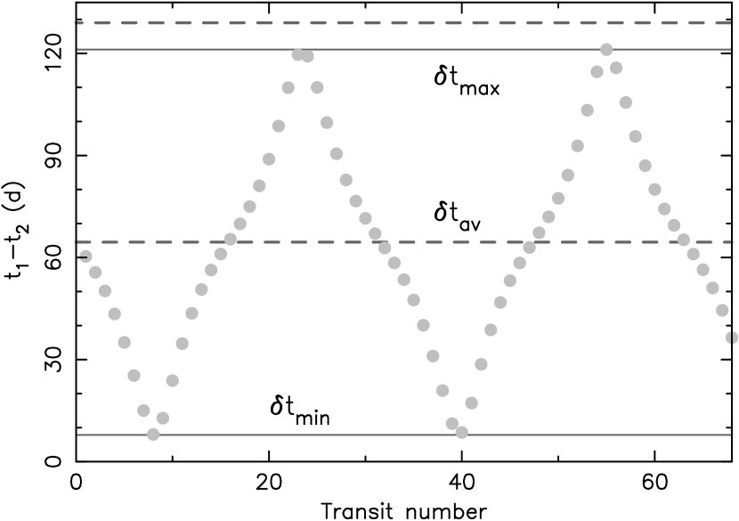
Figure 8: Difference between the transit time $t_{1}$ of the more massive planet and the immediately preceding transit time $t_{2}$ of the less massive planet in the simulation shown in Fig. 3. The abscissa is a transit number of the first planet. The average value of $t_{2}-t_{1}$, shown here as $\delta t_{\rm av}$, is half of the mean orbital period of the planets. The minimum and maximum values of $t_{2}-t_{1}$, shown here as $\delta t_{\rm min}$ and $\delta t_{\rm max}$, correspond to the extreme configurations, when $\theta=\lambda_{1}-\lambda_{2}$ is either minimum or maximum.

So far we discussed properties of TTVs obtained for the two planets. This is because these series rely on transit observations of each of the planets individually. While we have seen that a more complete information could be obtained when we have TTVs for both planets, some constraints were available even if transits of the larger planet are observed only. We now return to the ideal case, when transits of both planets are observed and note that even more complete information may be obtained by combining transit series of both planets. Consider a series of transit instants $t_{2}$ of the second (less massive, say) planet and the consecutive transit instants $t_{1}$ of the first planet. We may then construct a series of their difference $t_{1}-t_{2}$ as a function of the transit number. Using our example system from above, this information is shown in Fig. 8. As expected, $t_{1}-t_{2}$ has the characteristic triangular, sawtooth shape which basically follows from the time dependence of the planets’ angular separation $\theta(t)$ and spans values between zero and mean orbital period of the planets. Consequently, the minimum value of $t_{1}-t_{2}$, which we denote $\delta t_{\rm min}$, is directly related to the minimum angular separation $\theta_{\rm min}$ of the planets. Similarly, the average value of $t_{1}-t_{2}$, say $\delta t_{\rm av}$, is one half the mean orbital period of the planets (and when $t_{1}-t_{2}\simeq\delta t_{\rm av}$, the planets are at opposition). As a result

$$\theta_{\rm min}/\pi=\delta t_{\rm min}/\delta t_{\rm av}\;.$$ (43)

Since $\delta t_{\rm min}$ and $\delta t_{\rm av}$ are in principle discerned from observations, $\theta_{\rm min}$ can be fairly well constrained as well. In the same way, the maximum value of $t_{1}-t_{2}$, say $\delta t_{\rm max}$, provides

$$\theta_{\rm min}/\pi=2-\delta t_{\rm max}/\delta t_{\rm av}\;.$$ (44)

As an example, $\theta_{\rm min}$ estimated from the series in Fig. 8 is $\simeq 21.9^{\circ}$, which is very close to the numerically obtained value of $\simeq 21.4^{\circ}$. With $\theta_{\rm min}$ constrained, we note that the TTVs analysis using Eq. (42) provides an independent, correlated constraint of $\theta_{\rm min}$ and the normalized sum of planetary masses $\sigma_{+}/m_{0}=(m_{1}+m_{2})/m_{0}$. Henceforth, $\sigma_{+}/m_{0}$ can be directly obtained. If combined with the information about their ratio $m_{1}/m_{2}$ discussed above, we finally note that individual planetary masses $m_{1}$ and $m_{2}$ (given in $m_{0}$ units) can be determined from the observations.

4 Conclusions

While still awaiting for the first confirmed exoplanetary coorbital configuration, we derived here simple parametric relations that could be revealed from the TTV series of a such a system. From all possible coorbital architectures we chose here the horseshoe case that provides TTVs having the most singular nature. This is because at the zero order one may consider this situation as two non-interacting planets that periodically switch their orbits around some mean distance $a_{0}$ from the star. Instead of sinusoidal in nature, the TTVs thus resemble a triangular-shaped series with the half-period $T$ of the coorbital motion.

In an ideal case, where TTVs of both planets are observed, we find that the characteristics of a complete-enough dataset of planetary transits may directly provide information about their masses. This is because the ratio of the TTV amplitudes constrains directly the ratio of the planetary masses. Additionally, time separation between the transits of the two planets allows to constrain their minimum angular separation $\theta_{\rm min}$ as seen from the star. This information, if combined with Eq. (42), then provides a constraint on the the sum $\sigma_{+}=m_{1}+m_{2}$ of the planet’s masses in units of the stellar mass $m_{0}$.

Even if TTVs of only larger coorbiting planet are observed, say, one may use Eq. (42) to relate the total mass of planets, $\sigma_{+}$, to their minimum angular separation $\theta_{\rm min}$. This only requires the data constrain $T$ and the mean orbital period $P_{0}$, or rather their ratio $T/P_{0}$. Since the available range of $\theta_{\rm min}$ value is limited for stable orbital configurations, the value $T/P_{0}$ itself roughly sets a possible range of planetary mass, allowing us to distinguish cases with Jupiter-mass planets as opposed to the super-Earth-mass planets participating in the coorbital motion.

References

- (1) Beaugé, C., & Nesvorný, D. 2012, ApJ, 751, 119(14pp)
- (2) Beaugé, C., Sándor, Zs., Érdi, B., & Süli, Á. 2007, AA, 463, 359
- (3) Cresswell, P., & Nelson, R. P. 2006, AA, 450, 833
- (4) Cresswell, P., & Nelson, R. P. 2009, AA, 493, 1141
- (5) Fleming, H.J., & Hamilton, D.P. 2000, Icarus, 148, 479
- (6) Ford, E.C., & Gaudi, B.S. 2006, ApJ, 652, L137
- (7) Ford, E.C., & Holman, M.J. 2007, ApJ, 664, L51
- (8) Funk, B., Dvorak, R., & Schwarz, R. 2013, Cel. Mech. Dyn. Astron., 117, 41
- (9) Giuppone, C.A., Beaugé, C., Michtchenko, T.A., & Ferraz-Mello, S. 2010, MNRAS, 407, 390
- (10) Giuppone, C.A., Benítez-Llambay, P., & Beaugé, C. 2012, MNRAS, 421, 356
- (11) Goździewski, K., Breiter, S., & Borczyk, W. 2008, MNRAS, 383, 989
- (12) Haghighipour, N., Capen, S., & Hinse, T.C. 2013, Cel. Mech. Dyn. Astron., 117, 75
- (13) Hadjidemetriou, J., & Voyatzis, G. 2011, Cel. Mech. Dyn. Astron., 111, 179
- (14) Hadjidemetriou, J., Psychoyos, D, & Voyatzis, G. 2009, Cel. Mech. Dyn. Astron., 104, 23
- (15) Laskar, J., & Robutel, P. 1995, Cel. Mech. Dyn. Astron., 62, 193
- (16) Laughlin, G., & Chambers, J.E. 2002, AJ, 124, 592
- (17) Lyra, W., Johansen, A., Klahr, H., & Piskunov, N. 2009, AA, 493, 1125
- (18) Moldovan, R., Matthews, J. M., Gladman, B., Bottke, W. F., & Vokrouhlický, D. 2010, ApJ, 716, 315
- (19) Nesvorný, D. 2009, ApJ, 701, 1116
- (20) Nesvorný, D., & Morbidelli, A. 2008, ApJ, 688, 636
- (21) Nesvorný, D., & Vokrouhlický, D. 2014, ApJ, submitted
- (22) Robutel, P., & Pousse, A. 2013, Cel. Mech. Dyn. Astron., 117, 17
- (23) Rodríguez, A., Giuppone, C.A., & Beaugé, C. 2013, Cel. Mech. Dyn. Astron., 117, 59
- (24) Rowe, J. F., et al. 2006, ApJ, 646, 1241
- (25) Schwarz, R., Süli, Á., & Dvorak, R. 2009, MNRAS, 398, 2085
- (26) Sicardy, B., & Dubois, V. 2003, Cel. Mech. Dyn. Astron., 86, 321
- (27) Yoder, C.F., Colombo, G., Synnott, S.P., & Yoder, K.A. 1983, Icarus, 53, 431