Finite-temperature orbital-free DFT molecular dynamics:
coupling Profess and Quantum Espresso

Abstract

Implementation of orbital-free free-energy functionals in the Profess code and the coupling of Profess with the Quantum Espresso code are described. The combination enables orbital-free DFT to drive ab initio molecular dynamics simulations on the same footing (algorithms, thermostats, convergence parameters, etc.) as for Kohn-Sham (KS) DFT. All the non-interacting free-energy functionals implemented are single-point: the local density approximation (LDA; also known as finite-T Thomas-Fermi, ftTF), the second-order gradient approximation (SGA or finite-T gradient-corrected TF), and our recently introduced finite-T generalized gradient approximations (ftGGA). Elimination of the KS orbital bottleneck via orbital-free methodology enables high-T simulations on ordinary computers, whereas those simulations would be costly or even prohibitively time-consuming for KS molecular dynamics (MD) on very high-performance computer systems. Example MD simulations on H over a temperature range $2,000$ K $\leq\mathrm{T}\leq 4,000,000$ K are reported, with timings on small clusters (16-128 cores) and even laptops. With respect to KS-driven calculations, the orbital-free calculations are between a few times through a few hundreds of times faster.

I Introduction

Orbital-free density functional theory (OF-DFT) in principle provides an exact quantum-mechanical description of many-electron systems, both in the ground-state and at non-zero temperature T. Computationally, OF-DFT should be drastically less expensive than conventional Kohn-Sham (KS) DFT KohnSham at all T. The reason is well-known. Explicit use of the KS orbitals involves orthogonalization, which causes a computational cost scaling no better than $N_{b}^{3}$, with $N_{b}$ the number of occupied KS energy levels. At T=0 K, $N_{b}$ is proportional to the number of electrons in the system, hence grows with system size and complexity. Non-zero T makes matters worse, as the Fermi-Dirac distribution increases the number of computationally significant (compared to machine precision) occupation numbers relative to the ground state. Thus, the use of KS-DFT to drive ab initio molecular dynamics (AIMD) Barnett93 , MarxHutter2000 , Tse2002 , MarxHutter2009 , Kuhne12 is circumscribed by computer resource limits CollinsCECAM2012 , GerickePNP14 because a KS-DFT calculation must be done at each MD step. This scaling behavior is a notable challenge to detailed computational exploration of warm dense matter (WDM), which has temperatures of hundreds of kK at material densities from near ambient to several-fold compression. In contrast, the OF-DFT computational cost should scale essentially linearly with system size, irrespective of T.

Nevertheless, the KS decomposition is the appropriate framework for formulating OF-DFT as a useful computational tool for several reasons. Both the exchange (X) energy and the kinetic energy (KE) contribution to the DFT correlation (C) energy are defined in terms of the KS decomposition. And nearly 50 years of development of effective approximate XC functionals has taken place in that framework. The main ingredient, therefore, of ground-state OF-DFT is the non-interacting (or KS) KE functional. For non-zero T, the corresponding ingredient is the non-interacting free-energy functional, with contributions from the non-interacting KE and non-interacting entropy. Both ground-state and finite-T also require an orbital-free XC functional, of course.

Though the OF-DFT Euler equation can be cast quite easily into the form of a one-orbital (proportional to the square root of the density) KS equation with an extra potential, use of a standard KS code to solve that equation is not a viable strategy ChanCohenHandy2001 , KarasievTrickeyCPC2012 . Direct minimization techniques are required. Profess Ho..Carter08 , Hung..Carter10 is the only widely distributed OF-DFT computational package of which we are aware AbInitandNWChem which provides such techniques for computation of the ground state energy, electron density, inter-atomic electronic forces, and stress tensor with both periodic and Dirichlet boundary conditions (PBCs and DBCs). Profess may be used at a single ionic geometry (“single-point calculations”), wherein the total energy is minimized with respect to the electron density by one of the direct optimization methods implemented in the code, such as nonlinear conjugate gradient (CG) minimization and the truncated Newton (TN) method (see Ho..Carter08 for details and references) or for geometry optimization to find energetically optimal ion positions and cell vectors.

Profess is designed, however, as a ground-state OF-DFT code for optimization of two-point KE functionals containing a non-local part,

$$T_{\mathrm{NL}}[n]=\int\,d{\mathbf{r}}d{\mathbf{r}}^{\prime}n^{\lambda}({\mathbf{r}})K_{\mathrm{s}}[n({\mathbf{r}}),n({\mathbf{r}}^{\prime}),{\mathbf{r}},{\mathbf{r}}^{\prime}]n^{\gamma}({\mathbf{r}}^{\prime})\,.$$ (1)

Here $n({\mathbf{r}})$ is the electron number density, $\lambda+\gamma=8/3$, and the dimensionless kernel $K_{\mathrm{s}}[n({\mathbf{r}}),n({\mathbf{r}}^{\prime}),{\mathbf{r}},{\mathbf{r}}^{\prime}]$ is a type of response function. Commonly the non-local form Eq. (1) is used in conjunction with the Thomas-Fermi (TF) Thomas , Fermi , and von Weizsäcker Weizsacker functionals to give the approximate KS KE functional, $T_{\mathrm{s}}$:

$$T_{\mathrm{s}} \approx T_{\mathrm{TF}}+T_{\mathrm{W}}+T_{\mathrm{NL}}$$ (2)

$$T_{\mathrm{TF}}[n] = \int d{\mathbf{r}}\tau_{0}^{\mathrm{TF}}(n)$$ (3)

$$\tau_{0}^{\mathrm{TF}}(n) := \frac{3}{10}(3\pi^{2})^{2/3}n^{5/3}\equiv c_{\mathrm{TF}}n^{5/3}$$ (4)

$$T_{\mathrm{W}}[n] := \frac{1}{8}\int d{\mathbf{r}}\frac{|\nabla n({\mathbf{r}})|^{2}}{n({\mathbf{r}})}\equiv\int d{\mathbf{r}}t_{0}^{\mathrm{W}}([n];{\mathbf{r}})$$ (5)

(We use Hartree a.u. unless explicitly noted to the contrary. 1 E_H = 27.2116 eV, 1 bohr = 0.529177 Å.) The literature of such two-point approximations is accessible through Refs. Ho..Carter08, , Hung..Carter10, as well as the earlier review article by Wang and Carter WangCarter2000 .

In the interest of computational speed for AIMD, our work has emphasized one-point functionals. As distributed, the only one-point functionals included in Profess are $T_{\mathrm{TF}}$ and an empirically parametrized linear combination,

$$T_{\mathrm{TFvW}\{\lambda,\mu\}}=\lambda T_{\mathrm{TF}}+\mu T_{\mathrm{W}}\;,\;\\$$ (6)

with either the Thomas-Fermi ($\lambda=1$, $\mu=0$) or the von Weizsäcker ($\lambda=0$, $\mu=1$) term taken as the starting point and the other term assumed to be its correction.

Implementation of more refined one-point functionals in Profess, specifically our earlier T = 0 K generalized gradient approximation (GGA) kinetic energy functionals Perspectives , PRB80 , was reported without detail by two of us KarasievTrickeyCPC2012 . In addition to those earlier T = 0 K modifications, the enhanced version of Profess presented as a major part of this work includes our recently published GGA non-interacting free-energy functionals KarasievSjostromTrickey12A , VT84F and a new explicitly T-dependent XC functional LSDA-PIMC as well as two earlier ones PDW84 , PDW2000 .

All of these enhancements are in the context of coupling the modified Profess code to a fully-featured, freely available KS-AIMD code, Quantum Espresso QEspresso . The package of modifications and interfacing, called Profess@Q-Espresso, provides a new, finite-T OF-DFT-AIMD capability useful from the ground state to far into the WDM regime. Fig. 1 depicts the relationship between the two codes and the flow of calculation enabled by the new interface and associated modifications. Detailed commentary is below.

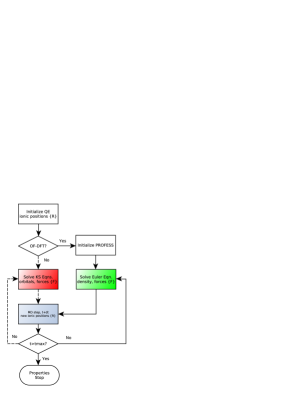
Figure 1: Flow chart for AIMD simulation with Profess$@$Q-Espresso package. Here $dt$ is the MD time step and $t_{\mathrm{max}}$ is the total simulation time.

Motivation for the combination is straight-forward. Whether the AIMD is KS-based or OF-DFT-based, the combination means that the same algorithms are used to execute the MD and to thermostat it in the NVT ensemble. For functional development work, this artifact-free uniformity of treatment is important. For materials simulation research generally, the Profess@Q-Espresso package makes up-to-date OF-DFT functionals and optimization techniques available to those who presently run KS-AIMD calculations, again on a uniform, artifact-free basis OurFrontiersInWDM.2014 . Third, use of packages such as Profess and Quantum Espresso which have published source code avoids wasteful duplication of software development effort.

The remainder of the presentation is organized as follows. Essentials (for this discussion) of finite-T OF-DFT are described in the next Section. Section III gives expressions for the ground state KE and finite-T non-interacting free-energy functionals implemented in the code, along with their functional derivatives and stress tensor components. Sect. IV provides the corresponding information for the XC functionals. Section V describes implementation issues, including the local model potentials required in OF-DFT, the patches needed, and the interface itself. Sect. VI gives example timings for OF-DFT static and AIMD calculations on Hydrogen.

II Finite-T OF-DFT Essentials

For fixed ionic positions $\{{\mathbf{R}}\}$, the grand canonical potential of a system with average electron number $N$ at temperature $\rm T$ and chemical potential $\mu$ may be expressed as the density functional Mermin65 , Stoitsov88

$$\Omega[n]={\mathcal{F}}[n]+\int d{\mathbf{r}}n({\mathbf{r}})\,\{v_{\mathrm{ext}}({\mathbf{r}})-\mu\}+E_{\rm{ion}}(\{{\mathbf{R}}\})\,,$$ (7)

where $v_{\mathrm{ext}}({\mathbf{r}})$ is the external potential and $E_{\rm{ion}}(\{{\mathbf{R}}\})$ is the ion-ion Coulomb repulsion energy. (For notational simplicity, explicit T-dependence is suppressed except where necessary.) The universal free-energy functional ${\mathcal{F}}[n]$

$${\mathcal{F}}[n]={\mathcal{F}}_{\mathrm{s}}[n]+{\mathcal{F}}_{\mathrm{H}}[n]+{\mathcal{F}}_{\mathrm{x}c}[n]\,.$$ (8)

has the conventional KS decomposition into the non-interacting free energy ${\mathcal{F}}_{\mathrm{s}}[n]$, (which has both kinetic and entropic contributions)

$${\mathcal{F}}_{\mathrm{s}}[n]={\mathcal{T}}_{\mathrm{s}}[n]-{\rm T}{\mathcal{S}}_{\mathrm{s}}[n]\,,$$ (9)

the classical Coulomb (or Hartree) interaction energy,

$${\mathcal{F}}_{\mathrm{H}}[n]=\tfrac{1}{2}\int\int d{\mathbf{r}}d{\mathbf{r}}^{\prime}\frac{n({\mathbf{r}})n({\mathbf{r}}^{\prime})}{|{\mathbf{r}}-{\mathbf{r}}^{\prime}|}\;.$$ (10)

The remainder, namely the difference between the interacting and non-interacting free-energy components plus the difference between the full quantum mechanical electron-electron interaction energy, ${\mathcal{U}}_{\rm ee}[n]$, and its classical part, ${\mathcal{F}}_{\rm H}[n]$, is the exchange-correlation (XC) free energy functional

$${\mathcal{F}}_{\mathrm{x}c}[n] \equiv ({\mathcal{T}}[n]-{\mathcal{T}}_{\mathrm{s}}[n])-{\mathrm{T}}({\mathcal{S}}[n]-{\mathcal{S}}_{\mathrm{s}}[n])$$ (11)

$$+({\mathcal{U}}_{\mathrm{e}e}[n]-{\mathcal{F}}_{\mathrm{H}}[n])\,.$$

By stipulation, the non-interacting (KS) system must deliver the same density as the interacting system, whence one has the KS effective potential $v_{\mathrm{K}S}$ and the system of coupled one-electron differential equations for the KS orbitals,

$$\left\{-\tfrac{1}{2}\nabla^{2}+v_{\rm KS}([n];{\mathbf{r}})\right\}\varphi_{j}({\mathbf{r}})=\varepsilon_{j}\phi_{j}({\mathbf{r}})\;$$ (12)

for the variational optimization. The KS potential is the sum of the external, $v_{\mathrm{ext}}$, Hartree, $v_{\rm H}:=\delta{\mathcal{F}}_{\rm H}[n]/\delta n$, and exchange-correlation, $v_{\mathrm{x}c}:=\delta{\mathcal{F}}_{\rm xc}[n]/\delta n$ contributions. In terms of the KS orbitals and Fermi-Dirac occupation numbers, the exact non-interacting KE and entropy are

$${\mathcal{T}}_{\mathrm{s}}[n] = \tfrac{1}{2}\sum_{j=1}^{\infty}f_{j}\int d{\mathbf{r}}\mid\nabla\varphi_{j}({\mathbf{r}})\mid^{2}$$ (13)

$${\mathcal{S}}_{\mathrm{s}}[n] = -k_{\mathrm{B}}\sum_{j=1}^{\infty}\{f_{j}\ln f_{j}+(1-f_{j})\ln(1-f_{j})\}\;.$$ (14)

The Fermi-Dirac occupation numbers are

$$f_{j}\equiv f(\varepsilon_{j}-\mu):=1/[1+\exp(\beta(\varepsilon_{j}-\mu))]\,,$$ (15)

$\beta:=1/k_{B}{\rm T}$, the electron number density is

$$n({\mathbf{r}})=\sum_{j=1}^{\infty}f_{j}|\varphi_{j}({\mathbf{r}})|^{2}\,,$$ (16)

and the average number of electrons is $N_{e}=\int d{\mathbf{r}}n({\mathbf{r}})$.

The orbital-free alternative has non-interacting free-energy and entropy functionals,

$${\mathcal{T}}_{\mathrm{s}}[n] = \int d{\mathbf{r}}\,\tau_{\mathrm{s}}[n]$$ (17)

$${\mathcal{S}}_{\mathrm{s}}[n] = \int d{\mathbf{r}}\,\sigma_{\mathrm{s}}[n]\;,$$ (18)

which depend explicitly upon the electron density (and its gradients, Laplacians, etc.) without explicit reference to the KS orbital manifold $\{\varphi\}$. Just as with the XC free energy functional, the exact form of those two functionals is unknown in general, so approximations must be constructed. Assuming that one has an orbital-free XC approximation as well, minimization of the functional Eq. (7) gives the single Euler equation

$$\frac{\delta{\mathcal{F}}_{\mathrm{s}}}{\delta n({\mathbf{r}})}=\mu-v_{\mathrm{K}S}([n];{\mathbf{r}})\equiv\mu([n];{\bf r})\,.$$ (19)

The XC contribution appears in $v_{\mathrm{K}S}$.

As noted already, solution of the OF-DFT problem is by direct minimization of the total electronic free energy

$$\mathcal{F}_{\mathrm{tot}}[n]=\mathcal{F}[n]+\int n(\mathbf{r})v_{\mathrm{ext}}(\mathbf{r})d\mathbf{r},$$ (20)

with the constraint that the integral of the density is constant. We use the nonlinear conjugate gradient techniques implemented in Profess. In contrast, the KS equation must be diagonalized in some basis, plane waves in the case of Quantum Espresso. Even with iterative diagonalization methods, the consequence is the computational time scaling bottleneck discussed already.

Another difference is that in KS calculations orbital-angular-momentum-dependent (usually called non-local) pseudopotentials commonly are used to great benefit. In OF-DFT one obviously cannot resort to such pseudopotentials; a local pseudopotential is required. Relevant consequences are discussed in Sect. V.

Whether by use of (12) or (19), once the variational minimum is obtained and $n$ is known for a specific ionic configuration, the electronic forces on the ions are calculated. In KS-AIMD this done via the Hellmann-Feynman theorem Feynman.1939 . In OF-DFT, the calculation is done directly from Perspectives

$${\mathbf{F}}_{I} = -\nabla_{{\mathbf{R}}_{I}}\Big{(}{\mathcal{F}}[n]+\int d{\mathbf{r}}\,v_{\mathrm{ext}}(\{{\mathbf{R}}\};{\mathbf{r}})n({\mathbf{r}})+E_{\mathrm{ion}}(\{{\mathbf{R}}\}]\Big{)}$$ (21)

$$= -\int d{\mathbf{r}}n({\mathbf{r}})\nabla_{{\mathbf{R}}_{I}}v_{\mathrm{ext}}(\{\mathbf{R}\};{\mathbf{r}})-\nabla_{{\mathbf{R}}_{I}}E_{\mathrm{ion}}(\{\mathbf{R}\})$$

$$- \int d{\mathbf{r}}\mbox{$\left[\vbox to14.0pt{}\right.$}\frac{\delta{\mathcal{F}}_{s}[n]}{\delta n({\bf r})}+v_{\rm KS}([n];{\bf r})\mbox{$\left]\vbox to14.0pt{}\right.$}\nabla_{{\mathbf{R}}_{I}}n({\bf r})\;.$$

At electronic equilibrium for a given ionic configuration, Eq. (19) is satisfied, so at constant volume the last integral becomes

$$\mu\int d{\mathbf{r}}\nabla_{{\mathbf{R}}_{I}}n({\mathbf{r}})=\mu\nabla_{{\mathbf{R}}_{I}}\int d{\mathbf{r}}n({\mathbf{r}})=\mu\nabla_{{\mathbf{R}}_{I}}N_{e}=0$$ (22)

which leaves

$${\mathbf{F}}_{I}=-\int d{\mathbf{r}}n({\mathbf{r}})\nabla_{{\mathbf{R}}_{I}}v_{\mathrm{ext}}(\{\mathbf{R}\};{\mathbf{r}})-\nabla_{{\mathbf{R}}_{I}}E_{\mathrm{ion}}(\{\mathbf{R}\})\;.$$ (23)

The corresponding contributions to the stress tensor are

$$\Sigma_{\alpha\beta}=\frac{1}{V}\sum_{\nu}\frac{\partial\Omega[n]}{\partial h_{\alpha\nu}}h_{\beta\nu}\,,$$ (24)

where $\alpha$, $\beta$ and $\nu$ are coordinate indices, $h$ is a matrix constructed from the cell vectors, and $V$ is the cell volume (see Ho..Carter08 ). Immediately the pressure follows as

$$P=-\frac{1}{3}\mathrm{Tr}\Sigma\;.$$ (25)

III Non-interacting free energy functionals

Here we describe our modifications of Profess to implement finite-T functionals, including GGA non-interacting and XC free-energy functionals, their functional derivatives, and stress-tensor contributions.

III.1 Finite temperature Thomas-Fermi

The LDA non-interacting free-energy is the finite-T TF functional Feynman..Teller.1949

$${\mathcal{F}}_{\mathrm{s}}^{\mathrm{TF}}[n]=\int d\mathbf{r}f_{\mathrm{s}}^{\mathrm{TF}}(n(\mathbf{r}),{\mathrm{T}})\;,$$ (26)

where

$$f_{\mathrm{s}}^{\rm TF}(n,{\rm T}) = \tau_{0}^{\mathrm{TF}}(n)\kappa(t)\,.$$ (27)

The zero-T TF kernel, $\tau_{0}^{\mathrm{TF}}(n)$, was defined at Eq. (4). The factor $\kappa(t)$, which is a combination of Fermi-Dirac integrals Bartel..Durand.1985 , is a dimensionless function of the reduced temperature

$$t={\mathrm{T}}/{\mathrm{T}}_{\mathrm{F}}:=\frac{2}{\beta[3\pi^{2}n({\mathbf{r}})]^{2/3}}\,.$$ (28)

Details of the structure of $\kappa$ and its behavior are in Ref. KarasievSjostromTrickey12A, along with a high-precision fit to a computationally convenient analytical form (see Appendix A of KarasievSjostromTrickey12A ). The associated TF potential and stress tensor are

$$v^{\mathrm{TF}}_{\mathrm{s}}([n];{\mathbf{r}})\equiv\frac{\delta{\mathcal{F}}_{\mathrm{s}}^{\mathrm{TF}}[n]}{\delta n({\mathbf{r}})}=\frac{\partial\tau_{0}^{\mathrm{TF}}(n)}{\partial n}\kappa(t)+\tau_{0}^{\mathrm{TF}}(n)\kappa^{\prime}(t)\frac{\partial t}{\partial n}\,,$$ (29)

and

$$\Sigma_{\alpha\beta}^{\mathrm{TF}}=\frac{\delta_{\alpha\beta}}{V}\int d{\mathbf{r}}\Big{[}f_{\mathrm{s}}^{\mathrm{TF}}(n({\mathbf{r}}),{\mathrm{T}})-n({\mathbf{r}})v^{\mathrm{TF}}_{\mathrm{s}}([n];{\mathbf{r}})\Big{]}\,.$$ (30)

Primes indicate derivatives with respect to the corresponding arguments.

III.2 Finite-T SGA and GGA functionals

Well-behaved, non-interacting GGA free energy functionals have distinct KE and entropic contributions of the form KarasievSjostromTrickey12A

$${\mathcal{F}}_{\mathrm{s}}^{\mathrm{GGA}}[n,{\mathrm{T}}] = \int d{\mathbf{r}}\tau_{0}^{\mathrm{TF}}(n)\xi(t)F_{\tau}(s_{\tau})$$ (31)

$$- \int d{\mathbf{r}}\tau_{0}^{\mathrm{TF}}(n)\zeta(t)F_{\sigma}(s_{\sigma})\;.$$

Here

$$\xi(t) = \kappa(t)-t\frac{\partial\kappa(t)}{\partial t}$$

$$\zeta(t) = -t\frac{\partial\kappa(t)}{\partial t}\;.$$ (32)

$\kappa(t)$ is as before. $F_{\tau}$ and $F_{\sigma}$ are the non-interacting KE and entropic enhancement factors. They depend upon two distinct T-dependent reduced density gradients, namely

$$s_{\sigma}(n,\nabla n,t) = s(n,\nabla n)\Big{(}\frac{t{\rm d}\tilde{h}(t)/{\rm d}t}{\zeta(t)}\Big{)}^{1/2}\,,$$

$$s_{\tau}(n,\nabla n,t) = s(n,\nabla n)\Big{(}\frac{\tilde{h}(t)-t{\rm d}\tilde{h}(t)/{\rm d}t}{\xi(t)}\Big{)}^{1/2}\,$$ (33)

where

$$s(n,\nabla n)=\frac{1}{2(3\pi^{2})^{1/3}}\,\frac{|\nabla n|}{n^{4/3}}\;$$ (34)

is the reduced density gradient familiar from T = 0 K GGA XC functionals. The function $\tilde{h}$ in Eq. (33) is another combination of Fermi-Dirac integrals for which an analytical fit is provided in Appendix A of Ref. KarasievSjostromTrickey12A, .

Functionals of the form of Eq. (31) which we have added in Profess include:
(i) the purely non-empirical functional obtained via a new constraint-based parametrization scheme VT84F

$$F_{\tau}^{\mathrm{VT84F}}(s_{\tau}) = 1-\frac{\mu s_{\tau}^{2}e^{-\alpha s_{\tau}^{2}}}{1+\mu s_{\tau}^{2}}$$

$$+ (1-e^{-\alpha s_{\tau}^{m/2}})(s_{\tau}^{-n/2}-1)+\frac{5}{3}s_{\tau}^{2}$$

$$F_{\sigma}^{\mathrm{VT84F}}(s_{\sigma}) = 2-F_{\tau}^{\mathrm{VT84F}}(s_{\sigma})\,,$$ (35)

with $m=8$, $n=4$, $\mu=2.778$ and $\alpha=1.2965$;
(ii) the mildly empirical (from a small set of molecular data) two-parameter (KST2) KarasievSjostromTrickey12A functional

$$F_{\tau}^{\mathrm{KST2}}(s_{\tau}) = 1+\frac{C_{1}s_{\tau}^{2}}{1+a_{1}s_{\tau}^{2}}$$

$$F_{\sigma}^{\mathrm{KST2}}(s_{\sigma}) = 2-F_{\tau}^{\mathrm{KST2}}(s_{\sigma})\;;$$ (36)

with constants $C_{1}=2.03087$, $a_{1}=0.29424$;
(iii) the finite-T extension of the zero-T APBEK functional CFDS11 given by Eq. (36) with $C_{1}=0.23889$ and $a_{1}=C_{1}/0.804$ (see Ref. VT84F );
(iv) the finite-T extension of the Tran-Wesolowski TranWesolowski02 (TW) ground state functional, given by Eq. (36) with $C_{1}=0.2319$ and $a_{1}=0.2748$ (again see Ref. KarasievSjostromTrickey12A );
(v) the finite-T SGA, also known as the gradient-corrected TF model Perrot.1979 ,

$$F_{\tau}^{\mathrm{SGA}}(s_{\tau}) = 1+\mu^{\mathrm{SGA}}s_{\tau}^{2}$$

$$F_{\sigma}^{\mathrm{SGA}}(s_{\sigma}) = 2-F_{\tau}^{\mathrm{SGA}}(s_{\sigma})\;,$$ (37)

with $\mu^{\mathrm{SGA}}=5/27$;
(vi) the empirical combination of the von WeizsäckerWeizsacker functional, Eq. (5), and the finite-T Thomas-Fermi (ftVWTF) functional KarasievSjostromTrickey12A given again by Eq. (37) but with $\mu^{\mathrm{VWTF}}=5/3$ instead of $\mu^{\mathrm{SGA}}$.

The potential in the Euler equation that arises from any of the ${\mathcal{F}}_{\mathrm{s}}^{\rm GGA}$ functionals can be evaluated using the generic equation for the functional derivative of a functional dependent on $n$ and $\nabla n$:

$$v^{\mathrm{GGA}}_{\mathrm{s}}([n];{\mathbf{r}}) \equiv \frac{\delta{\mathcal{F}}_{\mathrm{s}}^{\mathrm{GGA}}[n]}{\delta n({\mathbf{r}})}$$ (38)

$$= \frac{\partial\tau_{0}^{\rm TF}(n)}{\partial n}\xi(t)F_{\tau}(s_{\tau})+\tau_{0}^{\rm TF}(n)\xi^{\prime}(t)\frac{\partial t}{\partial n}F_{\tau}(s_{\tau})+\tau_{0}^{\rm TF}(n)\xi(t)\frac{\partial F_{\tau}(s_{\tau})}{\partial s_{\tau}^{2}}\Big{(}\frac{\partial s_{\tau}^{2}}{\partial n}+\frac{\partial s_{\tau}^{2}}{\partial t}\frac{\partial t}{\partial n}\Big{)}$$

$$- \frac{\partial\tau_{0}^{\rm TF}(n)}{\partial n}\zeta(t)F_{\sigma}(s_{\sigma})+\tau_{0}^{\rm TF}(n)\zeta^{\prime}(t)\frac{\partial t}{\partial n}F_{\sigma}(s_{\sigma})+\tau_{0}^{\rm TF}(n)\zeta(t)\frac{\partial F_{\sigma}(s_{\sigma})}{\partial s_{\sigma}^{2}}\Big{(}\frac{\partial s_{\sigma}^{2}}{\partial n}+\frac{\partial s_{\sigma}^{2}}{\partial t}\frac{\partial t}{\partial n}\Big{)}$$

$$- \nabla\cdot\Big{(}\tau_{0}^{\rm TF}(n)\xi(t)\frac{\partial F_{\tau}(s_{\tau})}{\partial s_{\tau}^{2}}\frac{\partial s_{\tau}^{2}}{\partial\nabla n}-\tau_{0}^{\rm TF}(n)\zeta(t)\frac{\partial F_{\sigma}(s_{\sigma})}{\partial s_{\sigma}^{2}}\frac{\partial s_{\sigma}^{2}}{\partial\nabla n}\Big{)}\,.$$

Rather than writing a single complicated expression for $v^{\mathrm{GGA}}_{\mathrm{s}}$ and evaluating it in Profess, we take advantage of the structural commonality of all GGAs for the non-interacting free energy. The RHS of Eq. (38) shows that there are only four factors which depend on a specific GGA, $F_{\tau}$, $F_{\sigma}$, $\partial F_{\tau}/\partial s_{\tau}^{2}$, and $\partial F_{\sigma}/\partial s_{\sigma}^{2}$. All the other contributions are generic for GGAs, e.g. $\zeta$, $\partial t/\partial n$, $\partial s_{\tau}^{2}/\partial n$, etc. The code is constructed to evaluate both the four specific contributions and all the generic ones individually, then assemble the result. The last line of (38) is calculated in reciprocal space, then inverse Fourier transformed.

The ftGGA stress tensor components are

$$\Sigma_{\alpha\beta}^{\rm GGA} = \frac{\delta_{\alpha\beta}}{V}\int d{\mathbf{r}}\Big{[}f_{s}^{\rm GGA}([n];{\bf r})-n({\bf r})v^{\rm GGA}_{\mathrm{s}}([n];{\bf r})\Big{]}$$ (39)

$$- \frac{1}{V}\int d{\mathbf{r}}\Big{[}\Big{(}\tau_{0}^{\rm TF}(n)\xi(t)\frac{\partial F_{\tau}(s_{\tau})}{\partial s_{\tau}^{2}}\frac{\partial s_{\tau}^{2}}{\partial|\nabla n|}-\tau_{0}^{\rm TF}(n)\zeta(t)\frac{\partial F_{\sigma}(s_{\sigma})}{\partial s_{\sigma}^{2}}\frac{\partial s_{\sigma}^{2}}{\partial|\nabla n|}\Big{)}\frac{\nabla_{\alpha}n({\bf r})\nabla_{\beta}n({\bf r})}{|\nabla n|}\Big{]}\,,$$

where

$$f_{s}^{\mathrm{GGA}}([n];{\bf r})=\tau_{0}^{\rm TF}(n)\xi(t)F_{\tau}(s_{\tau})-\tau_{0}^{\mathrm{TF}}(n)\zeta(t)F_{\sigma}(s_{\sigma})$$ (40)

and $\alpha$ and $\beta$ are Cartesian coordinate indices.

IV Exchange-correlation free energy functionals

Both the Profess and Quantum Espresso packages have standard ground state LDA PZ81 and GGA PBE96 XC functionals implemented. For $T>$ 0 K, the explicit T-dependence of the XC free-energy may be important. See discussions in Refs. KarasievSjostromTrickey2012PRE, , BrownEtAl2013, . Our enhancements of Profess and Quantum Espresso, include three explicitly T-dependent XC functionals, though with the recent advent of the first one LSDA-PIMC , the other two may be mostly of value for checking against earlier literature.

IV.1 LDA parametrized from path-integral Monte Carlo data

Recently we and a co-author presented a finite-T local spin-density approximation (LSDA) XC free-energy functional LSDA-PIMC obtained via accurate parametrization of first principles restricted path-integral Monte Carlo simulation data for the 3D homogeneous electron gas at finite T. The XC free-energy per particle is given by a function of $(r_{\mathrm{s}},t)$, with $r_{\mathrm{s}}=(3/4\pi n)^{1/3}$, and $t$ defined by Eq. (28) for the spin-unpolarized case, and $t={\mathrm{T}}/{\mathrm{T}}_{\mathrm{F}}^{\mathrm{p}}\equiv\frac{2}{\beta[6\pi^{2}n({\mathbf{r}})]^{2/3}}$ for the fully spin-polarized case,

$$f_{\mathrm{xc}}^{\mathrm{u/p}}(r_{\mathrm{s}},t)=-\frac{1}{r_{\mathrm{s}}}\frac{\omega_{\mathrm{u/p}}a(t)+b_{\mathrm{u/p}}(t)r_{\mathrm{s}}^{1/2}+c_{\mathrm{u/p}}(t)r_{\mathrm{s}}}{1+d_{\mathrm{u/p}}(t)r_{\mathrm{s}}^{1/2}+e_{\mathrm{u/p}}(t)r_{\mathrm{s}}}\,,$$ (41)

where $\omega_{\mathrm{u}}=1$ and $\omega_{\mathrm{p}}=2^{1/3}$ for the spin-unpolarized and fully-polarized cases respectively. The functions $a(t)$ and $b_{\mathrm{u/p}}(t)-e_{\mathrm{u/p}}(t)$ are given in LSDA-PIMC . In the small-$r_{\mathrm{s}}$ limit, Eq. (41) reduces to the LSDA finite-T exchange defined by exact scaling relations for X and fitted in Ref. PDW84 , $f_{\mathrm{x}}^{\mathrm{u/p}}(r_{\mathrm{s}},t)=-\omega_{\mathrm{u/p}}a(t)/r_{\mathrm{s}}$. The corresponding XC functional derivative is

$$v_{\mathrm{xc}}^{\mathrm{u/p}}([n];{\mathbf{r}}) \equiv \frac{\delta\Big{(}\int d{\mathbf{r}}nf_{\mathrm{xc}}^{\mathrm{u/p}}(r_{\mathrm{s}},t)\Big{)}}{\delta n({\mathbf{r}})}=f_{\mathrm{xc}}^{\mathrm{u/p}}(r_{\mathrm{s}},t)$$ (42)

$$+ n\Big{[}\frac{\partial f_{\mathrm{xc}}^{\mathrm{u/p}}(r_{\mathrm{s}},t)}{\partial r_{\mathrm{s}}}\frac{\partial r_{\mathrm{s}}}{\partial n}+\frac{\partial f_{\mathrm{xc}}^{\mathrm{u/p}}(r_{\mathrm{s}},t)}{\partial t}\frac{\partial t}{\partial n}\Big{]}\,,$$

where $\partial r_{\mathrm{s}}/\partial n=-r_{\mathrm{s}}/3n$ and $\partial t/\partial n=-2t/3n$ independent of spin-polarization.

The stress tensor for the XC free-energy is given by the standard expression for an LDA XC functional

$$\Sigma_{\mathrm{xc},\alpha\beta}^{\mathrm{u/p}}=\frac{\delta_{\alpha\beta}}{V}\int d{\mathbf{r}}\Big{[}n({\mathbf{r}})f_{\mathrm{xc}}^{\mathrm{u/p}}(r_{\mathrm{s}},t)-n({\mathbf{r}})v^{\mathrm{u/p}}_{\mathrm{xc}}([n];{\mathbf{r}})\Big{]}\,.$$ (43)

Only the spin-unpolarized version of the functional given by Eq. (41) is implemented in our modifications of the current version of Profess and Quantum Espresso.

IV.2 RPA functional

The functional developed by Perrot and Dharma-wardana (PDW84) PDW84 for the fully unpolarized case combines finite-T parametrized LDA exchange (in the form of the small $r_{\mathrm{s}}$ limit of Eq. (41)) with correlation treated via the random-phase approximation (RPA). The X free energy per electron in that functional is defined as

$$f_{\mathrm{x}}^{\mathrm{PDW84}}(r_{\mathrm{s}},t)\equiv f_{\mathrm{x}}^{\mathrm{u}}(r_{\mathrm{s}},t)=-\frac{1}{r_{\mathrm{s}}}a(t)\,.$$ (44)

Perrot and Dharma-wardana also used the form of Eq. (44) to fit the corresponding exchange potential $v_{\mathrm{x}}$ independently. Elsewhere KST-PDW84 we have shown that for a consistent pressure calculation, such an independent fit of $v_{\mathrm{x}}$ should not be used. Rather, $v_{\mathrm{x}}$ should be calculated via direct evaluation of the functional derivative of the specified X functional via use of an equation that corresponds to Eq. (42). The PDW84 correlation contribution is

$$f_{\mathrm{c}}^{\mathrm{PDW84}}(r_{\mathrm{s}},t) = \epsilon_{\mathrm{c}}^{\mathrm{LDA}}(r_{\mathrm{s}})(1+c_{1}t+c_{2}t^{1/4})\exp(-c_{3}t)$$ (45)

$$- 0.425437~{}(t/r_{\mathrm{s}})^{1/2}$$

$$\times \tanh(1/t)\exp(-c_{4}/t)\,,$$

where the $c_{i}$ are explicit functions of $r_{\mathrm{s}}$ and $\epsilon_{\mathrm{c}}^{\mathrm{LDA}}(n)$ is the zero-T LDA correlation energy per electron given by the Vosko, Wilk, and Nusair (VWN) parametrization VWN80 or by the re-parametrized Hedin-Lunqvist (rHL) local form HL.1971 , McDDWG.1980 (see Eqs. (3.7), (3.9)-(3.10) of Ref. PDW84, ). The correlation potential is the functional derivative given again by the analogue of Eq. (42). The stress tensor for the PDW84 XC functional is given by the spin-unpolarized version of Eq. (43).

IV.3 Classical map functional

Ref. PDW2000, presented an XC free-energy functional (hereafter denoted PDW00) built by mapping between the quantum system of interest and a more tractable classical system. We have implemented that functional via the fits provided in Ref. PDW2000, for the XC free energy per electron. For completeness that fit is

$$f^{\rm PDW00}_{\rm xc}(r_{\mathrm{s}},\mathrm{T}) =(\varepsilon_{\rm xc}(r_{\mathrm{s}},0)-P_{1})/P_{2},$$ (46)

$$P_{1} =(A_{2}u_{1}+A_{3}u_{2})\mathrm{T}^{2}+A_{2}u_{2}\mathrm{T}^{5/2},$$ (47)

$$P_{2} =1+A_{1}\mathrm{T}^{2}+A_{3}\mathrm{T}^{5/2}+A_{2}\mathrm{T}^{3},$$ (48)

where $A_{1}$, $A_{2}$, $A_{3}$, $u_{1}$, and $u_{2}$ are functions of $r_{\mathrm{s}}$ (see definitions in Ref. PDW2000, ). In addition, $\varepsilon_{\rm xc}(r_{\mathrm{s}},0)$ is the zero-T XC LDA energy per particle given by the PZ parametrization of QMC results PZ81 . Also we have implemented the XC potential which follows from exact differentiation of Eq. 46 as

$$v_{\mathrm{x}c}^{\rm PDW00}(n({\mathbf{r}}),\mathrm{T}) \equiv \frac{\delta\Big{(}\int d{\mathbf{r}}n\,f_{\mathrm{x}c}^{\rm PDW00}(n,\mathrm{T})\Big{)}}{\delta n({\mathbf{r}})}$$

$$=f_{\mathrm{x}c}^{\rm PDW00}(n,\mathrm{T}) + n\,\frac{\partial f_{\mathrm{x}c}^{\rm PDW00}(n,\mathrm{T})}{\partial n}\,.$$ (49)

The stress tensor for the PDW00 functional again is given by the spin-unpolarized version of Eq. (43).

V Implementational Aspects

V.1 Local pseudopotentials

Efficient use of Fourier-based numerical methods in OF-DFT computation as well as alleviation of difficulties introduced by the bare Coulomb nuclear-electron interaction make it desirable to regularize the singular external potential $v_{\mathrm{ext}}$. In the KS context, regularization often is accomplished with non-local pseudopotentials. The essential feature of such potentials, for this discussion, is their explicit dependence upon atomic orbital angular momentum, which makes them intrinsically incompatible with OF-DFT. Local pseudopotentials (LPPs) are required. The LPPs in a reciprocal space representation used by Profess are described in Refs. Ho..Carter08, , Hung..Carter10, .

More recently, we have developed LPPs in both direct and reciprocal space for Li as described in Ref. KarasievTrickeyCPC2012, . A hydrogen LPP intended for finite-T WDM applications was developed and tested in Ref. KarasievSjostromTrickey12A, . It has the reciprocal space form of the Heine-Abarenkov model Heine.Abarenkov.1964 , Goodwin..Heine.1990 , namely

$$v_{\mathrm{HA}}(q) = \frac{-4\pi}{Vq^{2}}[(Z-Ar_{\mathrm{c}}){\,\cos}(qr_{\mathrm{c}})$$

$$+(A/q){\,\sin}(qr_{\mathrm{c}})]f_{\mathrm{H}A}(q)\;,$$

$$f_{\mathrm{H}A}(q) := \exp{(-(q/q_{\mathrm{c}})^{6})}\;.$$ (50)

The parameters for H are $r_{\mathrm{c}}=0.25$ bohr, $A=6.18$ hartree and $q_{\mathrm{c}}=29.97$ bohr^-1. The parameters for the Al atom, developed in Ref. Goodwin..Heine.1990, , are $r_{\mathrm{c}}=1.15$ bohr, $A=0.1107$ hartree and $q_{\mathrm{c}}=3.5$ bohr^-1. All of these LPPs are available for download web-QTP-PP . The reciprocal space form is incorporated in Profess$@$Q-Espresso.

V.2 Modifications of Profess

All of the functionals described in the foregoing Sections are implemented in our modification of the Profess code, version 2.0. A short description of the most important subroutines and functions added to the modified version is given in Table 1. A new keyword, TEMP {real}, defines TEMPerature in Kelvin. Also we found it useful, especially for warm dense matter simulations, to define a new input parameter, cellScale {real} at the end of the first section of the geometry (.ion) file, as follows:

%BLOCK LATTICE_CART
  ...
  ...
  ...
  cellScale
%END BLOCK LATTICE_CART

This parameter defines a scaling factor for all lattice vectors and for all atomic coordinates. Its default value is 1.0.

V.3 New XC functionals implemented in Quantum Espresso

We have implemented the explicitly T-dependent XC functionals described in the preceding Section in our modification of Quantum Espresso vers. 5.0.3. Table 2 lists the added subroutines and keywords. These functionals can be used in standard KS calculations (static or AIMD) with Quantum Espresso. Note that the exchange-correlation internal and entropic contributions for the KSDT functional based on the PIMC simulation data LSDA-PIMC , (input_dft=’KSDT’ keyword) are calculated separately and the energy contributions listed in the standard output are changed accordingly (see next Subsection for details).

Table 1: Description of new functions and subroutines implemented in the modified version of Profess vers. 2.0.

Keyword	Calculates	function/subroutine
KINE MCPBE2	PBE2 zero-T KE Perspectives , PRB80 and functional derivativeKarasievTrickeyCPC2012 .	mcPBE2PotentialPlus
— —	The associated stress tensor $\Sigma_{\alpha\beta}^{\mathrm{PBE2}}$.	mcPBE2Stress
KINE PBETW	TW zero-T KE TranWesolowski02 and functional derivativeKarasievTrickeyCPC2012 .	PBETWPotentialPlus
— —	The associated stress tensor $\Sigma_{\alpha\beta}^{\mathrm{TW}}$.	PBETWStress
— —	The function $f(y)$ and derivatives, function $h\equiv\tilde{h}/72$ and derivatives Perrot.1979 .	FPERROT and FPERROT2
KINE TTF	TF free energy, entropic contribution, and functional derivative.	TTF1PotentialPlus
— —	The associated stress tensor $\Sigma_{\alpha\beta}^{\mathrm{TF}}$.	TTF1Stress
KINE VT84F	VT84F VT84F free energy, entropic contribution, and functional derivative.	TVTPotentialPlus
	VT84F stress tensor.	TVTStress
KINE HVWTF &	SGA and VWTF free energy, entropic contribution, and functional	TPBE2PotentialPlus
PARA MU ’value’	derivative KarasievSjostromTrickey12A , with the second term in Eq. (37)
	multiplied by value of parameter $\mu$.
KINE KST2	KST2 KarasievSjostromTrickey12A free energy, entropic contribution, and functional derivative.
KINE PBETWF	TW free energy, entropic contribution, and functional derivative.
KINE APBEF	APBEF VT84F free energy, entropic contribution, and functional derivative.
	SGA, VWTF, KST2,TW, and APBEF stress tensor.	TPBE2Stress
EXCH KSDT	LDA XC free-energy based on PIMC simulation data LSDA-PIMC .	KSDTXCPotentialPlus
— —	LDA XC internal energy based on PIMC simulation data.	KSDT_EXC
— —	Stress tensor corresponding to LDA XC free-energy.	KSDTXCStress
EXCH PDWX+NONE	PDW84 exchange free energy.	PDWXPotentialPlus
EXCH ...+PD84	PDW84 correlation free energy .	PD84CPotentialPlus
EXCH PDW00XC	PDW00 exchange-correlation free energy.	PD00XCPotentialPlus
— —	PDW84 exchange contribution to the stress tensor.	PDWXStress
— —	PDW84 correlation contribution to the stress tensor.	PDWCStress
— —	PDW00 stress tensor.	PD00XCStress

Table 2: Description of new functions and subroutines implemented in Quantum Espresso vers. 5.0.3.

Keyword	Calculates	function/subroutine
input_dft=’KSDT’	LDA XC free-energy based on PIMC simulation data.	fxc_ksdt_0
	LDA XC internal energy based on PIMC simulation data.	exc_ksdt_0
input_dft=’TXC0’	PDW00 XC free-energy.	pdw00xc
input_dft=’PDWX+...’	PDW84 exchange free energy.	pdwx_t
input_dft=’...+PD84’	PDW84 correlation free energy.	pdw84
input_dft=’...+PDW0’	PDW00 correlation free energy.	pdw00

V.4 Profess$@$Q-Espresso interface

The implementation of Profess$@$Quantum Espresso uses the modified Profess compiled as an external library for Quantum Espresso. Profess@Q-Espresso requires standard input files for both the Quantum Espresso PWscf package and for Profess. In addition, for each step (ionic configuration) of an OF-DFT AIMD calculation, Profess is called from the Quantum Espresso PWscf main program via the interface instead of executing the normal KS procedure within PWscf. The first such call is special:

  ...
  IF(useofdft) THEN
    if(istep.eq.0) CALL create_ofdftgeom()
    CALL ofdft_driver()
  ENDIF
  ...

Here useofdft {logical} is a new keyword added in Namelist: CONTROL with default value useofdft=.false. The second if statement takes care of initialization of Profess upon its first use. The interface creates the Profess geometry input file, inp.ion, on the basis of input provided for Quantum Espresso. That file includes the description of the cell vectors, atom types, and intra-cell atom coordinates (see the subroutine create_ofdftgeom). Required initializations of Profess with data provided in the input file ofdft.inpt also are done at that first call.

At all subsequent MD steps, data exchange between Quantum Espresso and Profess via the interface is minimal. After each MD step, the current ionic (nuclear) coordinates $\{{\mathbf{R}}\}$ (tau_ofdft) and the number of atoms (nat) are passed to Profess from Quantum Espresso via the interface. Prior to the next OF-DFT AIMD step, the interface transmits the following items from Profess to Quantum Espresso: the current contributions to the total free energy (etot), electronic internal energy (einternel), stress-tensor components (in principle; at present it returns only the pressure pressure) and new Born-Oppenheimer forces $\{{\bf F}\}$ (force_ofdft) for the next step. All of this is achieved from ofdft_driver via

  ...
  CALL profess(nat,tau_ofdft,force_ofdft, &
               pressure,etot,einternel)
  ...

The flow of control was shown in Fig. 1. The ionic coordinates measured as fractions of cell constants (and denoted as fractional atomic coordinates) at each MD step are stored in the md.xyz file for subsequent visualization. Note that Quantum Espresso uses Rydberg atomic units, while Profess uses Hartree atomic units internally and reports results in eV and Ångstroms. The interface takes account of this unit system difference.

The modified version of Profess also may be compiled as a stand-alone package from the same source files. Doing so enables OF-DFT calculations for either single-point or static geometry optimization without need of the interface to Quantum Espresso. The new subroutines in the modified version have the same parallelization, implemented through domain decomposition using MPI, though it is a development version with some inefficiently implemented parts.

Because the implementation includes XC functionals with explicit temperature dependence, both the internal and entropic contributions of the XC free-energy are calculated and the output is changed correspondingly. Here is a sample of modified Quantum Espresso output during OF-DFT MD simulation with the KSDT T-dependent LSDA XC functional

  ...
 OFDFT: (kbar) P=   7192.78778379771
 OFDFT: (Ry) Fxc=  -96.3275434867815
 OFDFT: (Ry) Exc=  -106.396016259169
  ...
 kinetic energy (Ekin) =       156.27791852 Ry
 temperature           =    129523.89686036 K
 Ekin + Etot (const)   =       -28.87878502 Ry
 free energy Etot      =      -185.15670354 Ry
 EinternEl(PR)             =   -30.86970711 Ry
 Eint=Ekin + EinternEl(PR) =   125.40821141 Ry
 smearing contrib.(-TS)(PR)=  -154.28699643 Ry
  ...

Shown are values of the pressure P from electronic structure calculations (ideal gas ionic contribution is not included), XC free energy Fxc, XC internal energy Exc, ionic kinetic energy Ekin, ionic temperature, sum of ionic-kinetic and free-energy Ekin + Etot, free-energy Etot, internal energy EinternEl, sum of ionic-kinetic and internal energy Eint=Ekin + EinternEl and the entropic contribution corresponding to the non-interacting term $-\mathrm{T}\mathcal{S}_{\mathrm{s}}$ and XC contribution $\mathcal{F}_{\mathrm{xc}}-\mathcal{E}_{\mathrm{xc}}$. The output for Kohn-Sham MD with T-dependent XC has the same quantities in slightly different order. Calculation of internal XC contributions for the PDW84 and PDW00 T-dependent functionals is not implemented at present, hence the partition of the free-energy (Etot) into the internal (EinternEl) and entropic contributions (-TS) is not correct for these functionals; only the free energies Etot and Ekin + Etot have meaningful values.

V.5 User implementation

In addition to the added functions and subroutines already described, the down-loadable material for user implementation of these modifications includes a basic README file. It lists patches which are required in the two codes, describes precisely how to install them, and includes scripts to run a few example static, OF-DFT AIMD and KS AIMD calculations as basic tests.

An important technical oddity is that Profess and Quantum Espresso require distinct, incompatible versions of the Fourier transform package fftw fftw . Thus, the downloads include fftw version 2.1.5 modified specifically for use with Profess and to avoid multiple definition problems caused by simultaneous use of version 3.3 by Quantum Espresso.

VI Results and discussion

In this Section we illustrate use of these added capabilities with two examples. First are timing and scaling comparisons for static lattice aluminum in the face-centered cubic (fcc) phase. Second are timing and scaling comparisons for AIMD simulations of hydrogen with OF-DFT AIMD via Profess@Q-Espresso and KS AIMD with Quantum Espresso at temperatures up to ${\mathrm{T}}=4,000,000$ K. All parallelized benchmark calculations used the high-performance computing cluster (2.4-2.8 GHz AMD Opteron) at University of Florida. Serial tests were on a single 3.2 GHz Intel $i5$ CPU.

Procedural context is helpful for interpreting the results. In ordinary practice, we do the OF-DFT AIMD simulations on 8-32 cores. To complete 6,000 MD steps with 128 H atoms in the simulation cell on a $64\times 64\times 64$ numerical grid typically takes between a few hours and a few days depending on simulation details such as the CPU speed, number of cores, thermodynamic conditions, and the choice of functional. A KS AIMD simulation with the same number of steps on 32 cores for the same number of H atoms at material density 0.983 g/cm³ on a $3\times 3\times 3$ k-mesh at ${\mathrm{T}}=30,000$ K takes about one month. For $\Gamma$ point KS calculations at 125,000 K and 180,000 K, the corresponding timings are about one and two months respectively.

VI.1 Static calculations - scaling

Static OF-DFT calculations for fcc-Al were done with between 2048 and 62500 atoms in a supercell. These used the modified Profess code alone; the interface to Quantum-Espresso and Quantum-Espresso itself are un-needed. Figure 2 shows the wall-clock time as a function of number of atoms for the VT84F non-interacting free energy functional and the PZ ground-state XC functional. Calculations show almost linear scaling $O(N\ln N)$ with system size CPL.Carter.2009 . The computational time on 128 cores for a single density optimization with 32,000 atoms is about 17 hours. The lower panel of that figure shows the speedup in going from 64 to 128 cores; at 32,000 atoms the speedup is about 80% of optimal.

Figure 2: Upper panel: execution time for OF-DFT static calculations with VT84F non-interacting free-energy functional and PZ XC for fcc-Al at material density $\rho_{\rm Al}=2.70$ g/cm³ and electronic temperature ${\mathrm{T}}_{\mathrm{el}}=100$ K with 2048, 4000, 8788, 16383, 32000, and 62500 atoms in the supercell. Calculations used 1 node $\times$ 64 cores and 2 nodes $\times$ 64 cores of AMD Opteron 2.4 GHz CPUs. Lower panel: speedup from 64 to 128 cores as a function of number of atoms.

The super-linear speedup at 4000 atoms apparently is a consequence of being able to keep the relatively small problem primarily in cache, something which is not possible at 64 cores.

A significant sidelight is that the non-empirical APBEK non-interacting functional not only fails to predict physically meaningful results (no binding at T=0 K), it sometimes exhibits bad numerical convergence, apparently because of improper large-$s$ behavior VT84F . Our mildly empirical ground-state non-interacting functional PBE2 Perspectives and its finite-T extension KST2 KarasievSjostromTrickey12A do predict binding, but both also have worse numerical convergence than VT84F because of the same wrong large-$s$ limit.

VI.2 Ab initio molecular dynamics: scaling

We did OF-DFT AIMD and KS AIMD simulations for H again at material density 0.983 g/cm³ ($r_{s}=1.40$ bohr) with 128 atoms in the simulation cell using the NVT ensemble regulated by the Andersen thermostat. Maximum temperatures were 4,000,000 K and 181,000 K for OF-DFT and KS MD respectively. Some of the physical results (e.g. equation of state, pair-correlation functions, etc.) have been published VT84F and others will be published systematically elsewhere. Here the focus is on comparative computational performance.

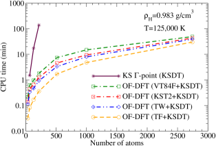
Figure 3: CPU time per MD step for OF-DFT calculations with VT84F, KST2, TF, and TW non-interacting free-energy functionals and PZ XC for H at material density $\rho_{\rm H}=0.983$ g/cm³ and ${\mathrm{T}}=125,000$ K with 32, 64, 128, 216, 512, 1000, and 2744 atoms in the simulation cell. Corresponding data for KS calculations with 64, 128 and 216 H atoms in the simulation cell ($\Gamma$-point) are shown for comparison. All calculations used a single core of an Intel $i5$ 3.2GHz CPU.

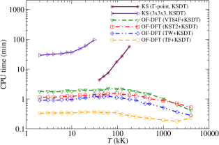
Figure 4: CPU time per MD step as a function of temperature for KS and OF-DFT calculations with VT84F, KST2, TF, and TW non-interacting free-energy functionals and PZ XC for H at material density $\rho_{\rm H}=0.983$ g/cm³ with 128 atoms in the simulation cell. All calculations used a single core of an Intel $i5$ 3.2GHz CPU.

Figure 3 compares OF-DFT and KS CPU time per MD step for hydrogen at ${\mathrm{T}}=125,000$ K as a function of the number of atoms $N$ in the simulation cell. All the timings are on a single core so as not to penalize the KS calculations for their serial overhead. OF-DFT AIMD exhibits almost linear scaling $O(N\ln N)$ with system size CPL.Carter.2009 , with 45 minutes of CPU time per MD step for $N=2744$. KS AIMD exhibits the expected approximately $N_{b}^{3}$ scaling, ($N_{b}>N$ is the number of thermally occupied one electron states). In the university context, that scaling makes such simulations prohibitively expensive for $N>216$ atoms.

CPU time as a function of temperature (still for $N=128$ hydrogen atoms in at material density 0.983 g/cm³) is shown in Figure 4. OF-DFT times vary slightly because of different convergence rates at different temperatures. For extremely high T, the CPU time decreases as the system tends toward the classical high-T limit. The KS CPU time per MD step in contrast increases drastically with increasing T because of the involvement of a growing number of partially occupied one-electron states $N_{b}$. Again, in our academic context, this temperature scaling makes KS AIMD for the given material density prohibitively expensive for T$>200,000$ K.

VI.3 Recommended functionals

Detailed accuracy comparisons among different orbital-free functionals and comparison between OF-DFT and reference KS results are outside the scope of the present work. Previous publications Perspectives , PRB80 , KarasievTrickeyCPC2012 , KarasievSjostromTrickey12A , VT84F provide relevant comparisons. For guidance in using the new interface and coding presented here, the main conclusions from those studies can be summarized as follows. (1) The standard non-interacting GGA functionals, including the empirical PBETW, and non-empirical APBEK ones, do not provide a qualitatively correct treatment of binding in simple molecules and in solids such as sc-H and fcc-Al. (2) In contrast, both the VT84F and PBE2/KST2 non-interacting functionals conversely provide at least semi-quantitatively correct predictions at all temperatures and have proper T=0 K limits. (3) The temperature dependence of the XC free energy becomes essential at elevated T. (4) The non-empirical VT84F functional provides almost identical results with those from the mildly empirical PBE2/KST2 and has the added benefit of better SCF convergence because of its correct large-$s$ behavior. On the basis of these facts, our current recommendation for OF-DFT AIMD calculations is to use the VT84F non-interacting free energy in combination with the KSDT XC free energy.

VII Conclusions

We have described the essential ingredients and modifications in our implementation of free energy functionals in the orbital-free Profess code. And we have described the interfacing of that code with the Quantum-Espresso code to provide a consistent suite with which to do both OF-DFT AIMD and KS AIMD calculations at all temperatures. Non-interacting free-energy one-point functionals defined within the finite-T generalized gradient approximation provide an adequate quantum statistical mechanical description of the electrons, thereby reducing the computational cost of using the non-local two-point (ground state) functionals in the original Profess code. Our Profess@Q-Espresso interface and all patches to Profess 2.0 and Quantum Espresso 5.0.3 are available by download from http://www.qtp.ufl.edu/ofdft and by request to the authors.

VIII Acknowledgments

VVK and SBT were supported by the U.S. Dept. of Energy TMS program, grant DE-SC0002139, as was the initial part of the effort by TS. The latter part of his work was supported by the Office of Fusion Energy Sciences of DOE. We acknowledge with thanks the provision of computational resources and technical support by the University of Florida High-Performance Computing Center.

References

- [1] W. Kohn and L.J. Sham, Phys. Rev. 140, A1133 (1965).
- [2] R.N. Barnett and U. Landman, Phys. Rev. B 48, 2081 (1993).
- [3] D. Marx and J. Hutter, “Ab initio molecular dynamics: Theory and Implementation”, in Modern Methods and Algorithms of Quantum Chemistry, J. Grotendorst, ed., John von Neumann Institute for Computing, (Jülich, NIC Series, Vol. 1, 2000) p. 301 and references therein.
- [4] J.S. Tse, Annu. Rev. Phys. Chem. 53, 249 (2002).
- [5] D. Marx and J. Hutter, Ab Initio Molecular Dynamics: Basic Theory and Advanced Methods (Cambridge University Press, Cambridge, 2009) and references therein.
- [6] T.D. Kühne, “Ab-Initio Molecular Dynamics” arXiv:1201.5945 [physics.chem-ph].
- [7] L.A. Collins (Los Alamos National Lab), “Equilibrium and Non-equilibrium Orbital-free Molecular Dynamics Simulations at Extreme Conditions”, CECAM Workshop, Paris, 05 Sept. 2012.
- [8] D.O. Gericke (Univ. Warwick) “Effective Interactions and Ion Dynamics in Warm Dense Matter”, Invited Talk I8, Physics of Non-ideal Plasmas 14, Rostock Germany, 11 Sept. 2012.
- [9] G. Kin-Lic Chan, A.J. Cohen, and N.C. Handy, J. Chem. Phys. 114, 631 (2001).
- [10] V.V. Karasiev and S.B. Trickey, Comput. Phys. Commun. 183, 2519 (2012).
- [11] G.S. Ho, V.L. Lignères, and E.A. Carter, Comput. Phys. Commun. 179, 839 (2008).
- [12] L. Hung, C. Huang, I. Shin, G.S. Ho, V.L. Lignères, and E.A. Carter, ∗ Comput. Phys. Commun. 181, 2208 (2010).
- [13] Version 7.6 of the AbInit code AbInit has what appears to be developer-level support of OF-DFT at the simplest finite-T Thomas-Fermi level. In private communication, E. Bylaska has informed us that some zero-T OF-DFT support is in the developer version of the periodic, plane wave package of the NWChem suite NWChem .
- [14] X. Gonze, B. Amadon, P.-M. Anglade, J.-M. Beuken, F. Bottin, P. Boulanger, F. Bruneval, D. Caliste, R. Caracas, M. Cote, T. Deutsch, L. Genovese, Ph. Ghosez, M. Giantomassi, S. Goedecker, D.R. Hamann, P. Hermet, F. Jollet, G. Jomard, S. Leroux, M. Mancini, S. Mazevet, M.J.T. Oliveira, G. Onida, Y. Pouillon, T. Rangel, G.-M. Rignanese, D. Sangalli, R. Shaltaf, M. Torrent, M.J. Verstraete, G. Zerah, and J.W. Zwanziger, Comput. Phys. Commun. 180, 2582 (2009); X. Gonze, G.-M. Rignanese, M. Verstraete, J.-M. Beuken, Y. Pouillon, R. Caracas, F. Jollet, M. Torrent, G. Zerah, M. Mikami, Ph. Ghosez, M. Veithen, J.-Y. Raty, V. Olevano, F. Bruneval, L. Reining, R. Godby, G. Onida, D.R. Hamann, and D.C. Allan, Zeit. Kristallogr. 220, 558 (2005).
- [15] M. Valieva, E.J. Bylaska, N. Govind, K. Kowalski, T.P. Straatsma, H.J.J. Van Dam, D. Wang, J. Nieplocha, E. Apra, T.L. Windus, W.A. de Jong, Comput. Phys. Commun. 181, 1477 (2010).
- [16] L.H. Thomas, Proc. Cambridge Phil. Soc. 23, 542 (1927).
- [17] E. Fermi, Atti Accad. Nazl. Lincei 6, 602 (1927).
- [18] C.F. von Weizsäcker, Z. Phys. 96, 431 (1935).
- [19] Y.A. Wang and E.A. Carter, “Orbital-free Kinetic-energy Density Functional Theory”, Chap. 5 in Theoretical Methods in Condensed Phase Chemistry, edited by S.D. Schwartz (Kluwer, NY, 2000) p. 117 and references therein.
- [20] V.V. Karasiev, S.B. Trickey, and F.E. Harris, J. Comput.-Aided Mat. Des. 13, 111 (2006).
- [21] V.V. Karasiev, R.S. Jones, S.B. Trickey, and F.E. Harris, Phys. Rev. B 80, 245120 (2009).
- [22] V.V. Karasiev, T. Sjostrom, and S.B. Trickey, Phys. Rev. B 86, 115101 (2012).
- [23] V.V. Karasiev, D. Chakraborty, O.A. Shukruto, and S.B. Trickey, Phys. Rev. B 88, 161108(R) (2013).
- [24] V.V. Karasiev, T. Sjostrom, J. Dufty, and S.B. Trickey, Phys. Rev. Lett. 112, 076403 (2014).
- [25] F. Perrot and M.W.C. Dharma-wardana, Phys. Rev. A 30, 2619 (1984).
- [26] F. Perrot and M.W.C. Dharma-wardana, Phys. Rev. B 62, 16536 (2000); F. Perrot and M.W.C. Dharma-wardana, Phys. Rev. B 67, 079901 (2003).
- [27] Paolo Giannozzi, Stefano Baroni, Nicola Bonini, Matteo Calandra, Roberto Car, Carlo Cavazzoni, Davide Ceresoli, Guido L. Chiarotti, Matteo Cococcioni, Ismaila Dabo, Andrea Dal Corso, Stefano de Gironcoli, Stefano Fabris, Guido Fratesi, Ralph Gebauer, Uwe Gerstmann, Christos Gougoussis, Anton Kokalj, Michele Lazzeri, Layla Martin-Samos, Nicola Marzari, Francesco Mauri, Riccardo Mazzarello, Stefano Paolini, Alfredo Pasquarello, Lorenzo Paulatto, Carlo Sbraccia, Sandro Scandolo, Gabriele Sclauzero, Ari P. Seitsonen, Alexander Smogunov, Paolo Umari, and Renata M. Wentzcovitch, J. Phys.: Condens. Matter 21, 395502 (2009).
- [28] V.V. Karasiev, T. Sjostrom, D. Chakraborty, J.W. Dufty, K. Runge, F.E. Harris, and S.B. Trickey, “Innovations in Finite-Temperature Density Functionals”, in Frontiers and Challenges in Warm Dense Matter, Series: Lecture Notes in Computational Science and Engineering, 96, edited by F. Graziani, M.P. Desjarlais, R. Redmer, and S.B. Trickey (Springer 2014), p. 61.
- [29] N.D. Mermin, Phys. Rev. 137, A1441 (1965).
- [30] M.V. Stoitsov and I.Zh. Petkov, Annals Phys. 185, 121 (1988).
- [31] R.P. Feynman, N. Metropolis, and E. Teller, Phys. Rev. 75, 1561 (1949).
- [32] J. Bartel, M. Brack, and M. Durand, Nucl. Phys. A445, 263 (1985).
- [33] L.A. Constantin, E. Fabiano, S. Laricchia, and F. Della Sala, Phys. Rev. Lett. 106, 186406 (2011).
- [34] F. Tran and T.A. Wesolowski, Int. J. Quantum Chem. 89, 441 (2002).
- [35] F. Perrot, Phys. Rev. A 20, 586 (1979).
- [36] J.P. Perdew, and A. Zunger, Phys. Rev. B 23, 5048 (1981).
- [37] J.P. Perdew, K. Burke, and M. Ernzerhof, Phys. Rev. Lett. 77, 3865 (1996); erratum Phys. Rev. Lett. 78, 1396 (1997).
- [38] V.V. Karasiev, T. Sjostrom, and S.B. Trickey, Phys. Rev. E 86, 056704 (2012).
- [39] E.W. Brown, B.K. Clark, J.L. DuBois, and D.M. Ceperley, Phys. Rev. Lett. 110, 146405 (2013).
- [40] L. Goodwin, R.J. Needs, and V. Heine, J. Phys.: Condens. Matter 2, 351 (1990).
- [41] V. Heine, and I.V. Abarenkov, Phil. Mag. 9, 451 (1964).
- [42] http://www.qtp.ufl.edu/ofdft/research/computation.shtml
- [43] R.P. Feynman, Phys. Rev. 56, 340 (1939); J. Hellman, Einf uhrung in die Quantenchemie (Deuticke and Company, Leipzig, 1937).
- [44] “Sensitivity of Pressure to the Accuracy of Evaluation of the Exchange-Correlation Free-energy Potential”, V.V. Karsiev, T. Sjostrom, and S.B. Trickey, U. Florida, March 2013 (unpublished).
- [45] S.H. Vosko, L. Wilk, and M. Nusair, Can. J. Phys. 58, 1200 (1980).
- [46] L. Hedin, and B.I. Lundqvist, J. Phys. C 4, 2064 (1971).
- [47] A.H. MacDonald, M.W.C. Dharma-wardana, and D.J.W. Geldart, J. Phys. F 10, 1719 (1980).
- [48] M. Frigio, and S.G. Johnson, Proc. IEEE 93, 216 (2005).
- [49] L. Hung, and E.A. Carter, Chem. Phys. Lett. 475, 163 (2009).