Maximizing the divergence from a hierarchical model of quantum states

Abstract.

We study many-party correlations quantified in terms of the Umegaki relative entropy (divergence) from a Gibbs family known as a hierarchical model. We derive these quantities from the maximum-entropy principle which was used earlier to define the closely related irreducible correlation. We point out differences between quantum states and probability vectors which exist in hierarchical models, in the divergence from a hierarchical model and in local maximizers of this divergence. The differences are, respectively, missing factorization, discontinuity and reduction of uncertainty. We discuss global maximizers of the mutual information of separable qubit states.

Divergence from a hierarchical model

Index Terms: many-party correlation, maximum-entropy principle, hierarchical model, irreducible correlation, mutual information, multi-information, factorization, discontinuity, maximizer, separable state

AMS Subject Classification: 62H20, 62F30, 94A17, 81P16, 81P45

1. Introduction

In this article we quantify many-party correlations in the state of a composite quantum system which can not be observed in subsystems composed of less than a given number of parties. One of us [4] has quantified stochastic interactions in terms of a distance from non-interacting states. Following this idea, we replace in the present context the non-interacting states by states which are fully described by their restriction to selected subsystems. For a definition of the latter states the maximum-entropy principle was suggested earlier [1, 31, 55] because it solves the inverse problem to reconstruct a global state from subsystem states and it offers also a natural scale of many-party correlation in terms of the gap to the maximal entropy value. Mathematical deduction leads from here to the conception [4, 1, 7, 56, 52] that many-party correlation should be quantified in terms of the divergence (which is an asymmetric distance) from a family of Gibbs states which we will call hierarchical model in the sense of [30].

We are considering a composite system of $N\in\mathds{N}$ units, parties, particles, etc. $[N]:=\{1,\ldots,N\}$. Tacitly, probability vectors on a finite space (classical case) are included in this discussion of quantum systems because vectors can be embedded as diagonal matrices into a matrix algebra (quantum case). We consider the algebra $\mathcal{M}_{d}$ of complex $d\times d$ matrices with identity $\mathds{1}_{d}$, $d\in\mathds{N}$, and we endow it with the Hilbert-Schmidt inner product $\langle a,b\rangle:={\rm tr}(ab^{*})$, $a,b\in\mathcal{M}_{d}$. Each unit $i\in[N]$ has a unit size $n_{i}\in\mathds{N}$ and a C*-subalgebra $\mathcal{A}_{i}\subset\mathcal{M}_{n_{i}}$ such that $\mathds{1}_{n_{i}}\in\mathcal{A}_{i}$. The composite system is described by the tensor product algebra $\mathcal{A}_{[N]}:=\mathcal{A}_{1}\otimes\cdots\otimes\mathcal{A}_{N}$.

The simplest notion of correlation is the total correlation. The corresponding set of states without any correlations is the space of tensor product states

(1.1) $$\mathcal{F}_{1}:=\{\rho_{1}\otimes\cdots\otimes\rho_{N}\mid\mbox{ $\rho_{i}$ is a quantum state of unit $i\in[N]$}\}.$$

Here a state of a quantum system with C*-algebra $\mathcal{A}\subset\mathcal{M}_{d}$, $d\in\mathds{N}$, denotes a density matrix which is a positive semi-definite matrix in $\mathcal{A}$ of unit trace [45]. We observe the following.

• The states in $\mathcal{F}_{1}$ are totally uncorrelated in the sense that the probability distribution of the measurement outcomes (with respect to a projective [35] or simple [2] measurement) of an observable $a_{1}\otimes\cdots\otimes a_{N}$ has the product form.

• Any distance of a quantum state from $\mathcal{F}_{1}$ quantifies correlations in the Aristotelian sense that the whole is more than the sum of its parts, cf. [4]. Here a distance should be zero for points in $\mathcal{F}_{1}$ and strictly positive otherwise.

It is interesting to differentiate correlations between the number of particles which interact. An algebraic generalization from no correlation (1.1) to $k$-party interaction, $k\in\mathds{N}$, is unknown in the quantum setting, although it exists classically as we recall in Sec. 2. The way out is the maximum-entropy principle [24] which also delivers a natural scale for correlations: In Sec. 1.1 we define a quantity $c_{k}(\rho)$ capturing all correlations in a state $\rho$ in $\mathcal{A}_{[N]}$ which can not be observed in any $k$-party subsystem. Later in Sec. 4 we introduce the notion of hierarchical model which allows to define interaction patterns of subsystems which are more general than the class of $k$-party subsystems.

Based on our earlier work [50, 51, 52, 53] we recall in Sec. 3 that the many-party correlation $c_{k}$ is just the divergence

(1.2) $$c_{k}(\rho)=\inf\{D(\rho,\sigma)\mid\sigma\in\mathcal{E}_{k}\},\quad\mbox{$\rho$ a state in $\mathcal{A}_{[N]}$}$$

from the Gibbs family

(1.3) $$\mathcal{E}_{k}:=\{e^{H}/{\rm tr}(e^{H})\mid H\in\mathcal{H}_{k}\}$$

of the $k$-local Hamiltonians $\mathcal{H}_{k}$. Here a $k$-local Hamiltonian [28, 17] is defined as a sum of tensor product terms $a_{1}\otimes\cdots\otimes a_{N}$ with at most $k$ non-scalar factors $a_{i}\in\mathcal{A}_{i}^{\operatorname{h}}$, $i\in[N]$, where $\mathcal{A}^{\operatorname{h}}$ denotes the real space of self-adjoint matrices in a C*-algebra $\mathcal{A}\subset\mathcal{M}_{d}$, $d\in\mathds{N}$. The Umegaki relative entropy which we call divergence is an asymmetric distance between states $\rho,\sigma$ in $\mathcal{M}_{d}$ defined by

$$D(\rho,\sigma):={\rm tr}\,\rho(\log(\rho)-\log(\sigma))$$

if the kernel of $\sigma$ is included in the kernel of $\rho$, otherwise $D(\rho,\sigma):=\infty$. The distance-like property of $D(\rho,\sigma)\geq 0$ with equality if and only if $\rho=\sigma$ is well-known [49, 35].

Related concepts in the literature include the notion of $k$-body potential in statistical mechanics [45] which is similar to the notion of $k$-local Hamiltonian. The proof of (1.2) that the correlation $c_{k}$ equals the divergence from $\mathcal{E}_{k}$ has been given in probability theory in [1, 7]. The quantum mechanical proof in [56] works only for states of maximal rank while the proof in [52] is valid without rank restriction.

Some new results are pointed out in Secs. 1.2 and 1.3. We remark in Sec. 1.2 that the step from maximal rank to non-maximal rank has a physical interpretation as a zero-temperature limit. This step entails phenomena like a missing factorization of maximum-entropy probability distributions and a discontinuity of quantum correlations. We do not know how reliable the algorithms [34] are at discontinuities of the divergence from $\mathcal{E}_{k}$. In Sec. 1.3 we address maximizers of correlation and we point out a curious reduction of uncertainty in quantum maximizers.

The Gibbs family $\mathcal{E}_{1}$ is known as the independence model and the divergence of a state $\rho$ in $\mathcal{A}_{[N]}$ from $\mathcal{E}_{1}$ quantifies the total correlation. We show in Sec. 5 that the divergence from $\mathcal{E}_{1}$ can be written in the form

(1.4) $$c_{1}(\rho)=H(\rho_{\{1\}})+\cdots+H(\rho_{\{N\}})-H(\rho)$$

where the $\rho_{\{i\}}$ are one-party marginals (Sec. 1.1) and

$$H(\sigma):=-{\rm tr}\sigma\log(\sigma)$$

denotes the von Neumann entropy of a state $\sigma$ in $\mathcal{M}_{d}$, $d\in\mathds{N}$. The right-hand side of (1.4) is also known as multi-information [6] and quantifies the number of random bits needed to erase all correlations between the units of a composite system [20] if the base of the logarithm is two.

Finally, we remark that the divergence from an exponential family plays a major role in the context of the maximum likelihood estimation [16]. The relative entropy of entanglement [48] is analogously defined in terms of the divergence from the convex set of non-entangled states. However, this set does not form an exponential family. Therefore this entanglement measure can not be motivated in terms of the maximum entropy principle, in contrast to the divergence representation (1.2) of the correlation quantity $c_{k}$. From the information-geometric perspective, it is more natural to apply the relative entropy projection onto a convex set with respect to the first argument of $D$, which is consistent with the work [10] on hypothesis testing.

1.1. Interaction patterns

The maximum-entropy principle, in its statistical inference view [24], is suitable to introduce particle numbers into quantum many-party correlations. If information about a state is available in the form of a constraint (imagine a subset containing the state) then the state which maximizes the von Neumann entropy $H$ under the constraint is considered [24] the least informative state representing the given information. Our constraints will be quantum marginals. Denoting the algebra of the subsystem of units in $\nu\subset[N]$ by the tensor product $\mathcal{A}_{\nu}:=\bigotimes_{i\in\nu}\mathcal{A}_{i}$ with identity $\mathds{1}_{\nu}$, the $\nu$-marginal $\rho_{\nu}$ of a state $\rho$ in $\mathcal{A}_{[N]}$ is defined by the equations

$$\langle\rho_{\nu},a\rangle=\langle\rho,a\otimes\mathds{1}_{[N]\setminus\nu}\rangle,\quad a\in\mathcal{A}_{\nu}.$$

If for some $k\in\mathds{N}$ the information consists of the marginals of all $k$-party subsystems, that is subsystems composed of $k$ units, of some global state $\rho$ in $\mathcal{A}_{[N]}$ then we notice

• any two states compatible with the constraint are indistinguishable on any subsystem composed of $k$ or less units;

• a state in $\mathcal{A}_{[N]}$ which is compatible with the constraint and has less entropy than the maximal entropy $H_{\max}$ has additional information.

Since $\rho$ is compatible with the constraint, it is natural to quantify the additional information in $\rho$ by $c_{k}(\rho):=H_{\max}-H(\rho)$. We take this information as a definition of many-party correlations: The quantity $c_{k}(\rho)$ captures all correlations in $\rho$ which can not be observed in any $k$-party subsystem.

We remark that the very closely related quantity of irreducible $k$-party correlation [31, 55] is defined by $C_{k}(\rho):=c_{k-1}(\rho)-c_{k}(\rho)$ and quantifies all correlations which can be observed in the $k$-party subsystems but not in the $(k-1)$-party subsystems. For example the irreducible three-party correlation $C_{3}$ can be used to distinguish the genuine 3-party correlation from 2-party correlation, like three-tangle in [13]. But entanglement is just one kind of quantum correlation, so the quantity $C_{3}$ is different from three-tangle. For the case of probability distributions see for example [26, 7].

1.2. Non-maximal rank phenomena

The step from maximal rank to non-maximal rank is crucial in ultra-cold physics, for example in condensed matter physics [46, 54] or adiabatic quantum computation [38], because non-maximal rank states are zero-temperature limits of Gibbs states in the sense of $e^{-\beta H}/{\rm tr}(e^{-\beta H})$ for $\beta\to\infty$. Mathematical phenomena of non-maximal rank appear in Sec. 2 in the context of higher factorization $\mathcal{F}_{1}\subset\cdots\subset\mathcal{F}_{N}$ by generalizing (1.1). Higher factorization is unknown in the quantum case but consequences may generalize from classical to quantum systems, who knows? We anticipate that the inclusions $\mathcal{E}_{k}\subset\mathcal{F}_{k}\subset\overline{\mathcal{E}_{k}}$ are strict ($\overline{\mathcal{E}_{k}}$ denotes norm closure) for $k\geq 2$. In a three-qubit quantum system it is known that the divergence from $\mathcal{E}_{2}$ is discontinuous at the GHZ state [52, 43]. This is indeed a very pronounced irregularity and related phenomena have been suggested as signatures of quantum phase transitions [12]. In the classical case the divergence from $\mathcal{E}_{k}$ is continuous for all $k\in\mathds{N}$ [51]. We will return to the continuity problem in Sec. 3.

1.3. Maximizing the divergence

We have studied maximizers of the divergence from Gibbs families in the classical case for example in [5, 6]. The latest result in the area is [41]. Two of us [53, 51] have shown that quantum maximizers have properties analogous to the following classical ones provided in [5]:

• A local maximizer of the divergence from a Gibbs family $\mathcal{E}$ is the conditional distribution of its projection to $\mathcal{E}$;

• a local maximizer of the divergence from $\mathcal{E}$ is supported on a set of size of at most $\dim_{\mathds{R}}(\mathcal{E})+1$.

We prove in Sec. 6 that the upper bound on the support size improves in the quantum setting to $\sqrt{\dim_{\mathds{R}}(\mathcal{E})+1}$ because the state space of an $n$-level quantum system has dimension $n^{2}-1$ compared to $n-1$ which is the dimension of the probability simplex. For example, if all $N\in\mathds{N}$ units of a composite system have the same unit size $n\in\mathds{N}$, then the independence model $\mathcal{E}_{1}$ has dimension $N(n-1)$ in the classical case and $N(n^{2}-1)$ in the quantum case of a full matrix algebra. Therefore, a local maximizer of the multi-information has support at most ${\mathcal{O}}(N)$ respectively ${\mathcal{O}}(\sqrt{N})$, see the paragraph of (6.6). In a loose analogy, if the classical bound was sharp, these bounds confirm that quantum systems are less uncertain than classical systems [9, 11]. In both cases we have an exponential reduction from the complete randomness with corresponding support size $n^{N}$.

Global maximizers are less coherent in the classical-quantum comparison. The classification of global maximizers of the multi-information [6] in the classical setting is not valid in the quantum setting due to the entanglement. However, we demonstrate in Sec. 7 that the methods in [6] are helpful to understand maximizers of the mutual information of separable qubit states.

2. Factorization of probability distributions

We recall from [19, 18] that the set of probability vectors with at most $k$-party interactions has several algebraic representations. Loopholes in the representations are explained by examples from [25] and by proving their minimality.

Let us associate to each unit $i\in[N]$ a state space $X_{i}$ which is an arbitrary set of cardinality equal to the unit size $n_{i}$ defined earlier. The composite system has the state space $X_{1}\times\cdots\times X_{N}$. For any subset $\nu\subset[N]$ we consider a subsystem $X_{\nu}:=\bigtimes_{i\in\nu}X_{i}$ and for any tuple $x=(x_{1},\ldots,x_{n})\in X_{[N]}$ its restriction $x_{\nu}:=(x_{i})_{i\in\nu}$ to the subsystem. We denote the probability simplex over a finite set $X$ by

$$\textstyle\Delta(X):=\{p\in\mathds{R}^{X}\mid\forall i\in X:p(i)\geq 0,\sum_{i\in X}p(i)=1\}.$$

When switching to the notation of quantum systems in Sec. 1 we tacitly identify $\mathds{C}^{X\nu}\cong\mathcal{A}_{\nu}$ for subsets of units $\nu\subset[N]$. Then $\Delta(X_{\nu})$ is the set of states in $\mathcal{A}_{\nu}$.

A probability vector $p\in\Delta(X_{[N]})$ factorizes with respect to $k$-party subsystems, $k\in\mathds{N}$, if there are functions $\psi_{\nu}\in\mathds{R}^{X_{\nu}}$, $\nu\subset[N]$, $|\nu|=k$, such that

(2.1) $$\textstyle p(x)=\prod_{\nu\subset[N],|\nu|=k}\psi_{\nu}(x_{\nu}),\quad x\in X_{[N]}.$$

Let us denote by $\mathcal{F}_{k}$ the set of all probability vectors with (2.1). Notice that the definition of $\mathcal{F}_{1}$ is consistent with (1.1) in the classical case.

We follow [19] by working out Lemma 2.1. Thereby we meet two representations of $\mathcal{F}_{k}$. The lemma is a condition for the inclusion of a probability vector into $\mathcal{F}_{k}$ in terms of the support. Using the set of $k$-party subsystem states $I_{k}:=\bigcup_{\nu\subset[N],|\nu|=k}\{(\nu,x)\mid x\in X_{\nu}\}$ we define a matrix with rows indexed by $I_{k}$ and columns indexed by $X_{[N]}$

(2.2) $$a_{(\nu,y),x}:=\left\{\begin{array}[]{rl}1&\text{if }x_{\nu}=y\\ 0&\text{else}\end{array}\right.,\quad(\nu,y)\in I_{k},x\in X_{[N]}.$$

See Example 2.2 for three bits and $k=2$. Notice for all $x\in X_{[N]}$ that $\sum_{i\in I_{k}}a_{i,x}={N\choose k}$ holds. The matrix (2.2) defines a monomial map

$$\Phi:[0,\infty)^{I_{k}}\to[0,\infty)^{X_{[N]}},\quad t\mapsto(\textstyle\prod_{i\in I_{k}}t(i)^{a_{i,x}})_{x\in X_{[N]}}$$

where we agree on $0^{0}=1$ and $0^{\alpha}=0$ for $\alpha>0$. It is easy to prove for $p\in\Delta(X_{[N]})$ that $p$ lies in $\mathcal{F}_{k}$ if and only if $p$ belongs to the image of $\Phi$. To get a second representation of $\mathcal{F}_{k}$ we define a family of functions $r_{\theta}(x):=\exp(\sum_{i\in I_{k}}\theta(i)a_{i,x})$, $x\in X_{[N]}$, with family parameter $\theta\in[-\infty,\infty)^{I_{k}}$. If $\theta\in[-\infty,\infty)^{I_{k}}$ satisfies the condition

(2.3) $$\textstyle r_{\theta}(x)>0\mbox{ holds for at least one }x\in X_{[N]}$$

then a probability vector $p_{\theta}:=Z(\theta)^{-1}r_{\theta}$ is defined where $Z(\theta)$ is for normalization. It is easily proved that the set of constructed probability vectors $p_{\theta}$ is the intersection of $\Delta(X_{[N]})$ with the image of $\Phi$.

The support of a vector $v\in\mathds{R}^{X}$ indexed by a finite set $X$ is defined by ${\rm supp}(v):=\{x\in X\mid v(x)\neq 0\}$. The column of the matrix (2.2) with column label $x\in X_{[N]}$ will be written $a_{x}:=(a_{i,x})_{i\in I_{k}}$. We call a non-empty subset $F\subset X_{[N]}$ $k$-feasible [19] if

$$\textstyle{\rm supp}(a_{x})\not\subset\bigcup_{y\in F}{\rm supp}(a_{y})\quad\mbox{holds for all }x\in X_{[N]}\setminus F.$$

It is easy to see that a non-empty subset $F\subset X_{[N]}$ is $k$-feasible if and only if $F$ is the support set of a vector $r_{\theta}(x)$ for some $\theta\in[-\infty,\infty)^{I_{k}}$ satisfying (2.3). Restriction to $\theta\in\{-\infty,0\}^{I_{k}}$ gives the following.

Lemma 2.1.

The uniform probability vector supported on a non-empty subset $F\subset X_{[N]}$ belongs to $\mathcal{F}_{k}$ if and only if $F$ is $k$-feasible.

Notice that (2.3) implies inclusions between $\mathcal{F}_{k}$ and the Gibbs family $\mathcal{E}_{k}$ of the $k$-local Hamiltonians (1.3):

(2.4) $$\mathcal{E}_{k}\subset\mathcal{F}_{k}\subset\overline{\mathcal{E}_{k}}.$$

We recall a representation of $\overline{\mathcal{E}_{k}}$ in Thm. 3.2 in [19] (unknown in the quantum case) where $\overline{\mathcal{E}_{k}}$ is the intersection of the probability simplex $\Delta(X_{[N]})$ and of a non-negative toric variety defined as the set of all vectors $s\in[0,\infty)^{X_{[N]}}$ such that we have

$$\textstyle\prod_{x\in X_{[N]}}s(x)^{u(x)}=\prod_{x\in X_{[N]}}s(x)^{v(x)}$$

for all $u,v\in\mathds{N}_{0}^{X_{[N]}}$ where $u-v$ lies in the kernel of the matrix (2.2).

Let us give an example to see why $\mathcal{F}_{k}$ is not closed for $k\geq 2$ and let us prove minimality of the example.

Example 2.2.

Let $k,N\in\mathds{N}$ and $N>k\geq 2$. Then $\overline{\mathcal{E}_{k}}\setminus\mathcal{F}_{k}$ is non-empty. For simplicity we consider $N=k+1$ bits. The subset

$$Y:=\{(x_{1},\ldots,x_{N})\mid x_{i}=0\text{ for all but one }i\in[N]\}$$

of $X_{[N]}=\{0,1\}^{N}$ is not feasible. So Lemma 2.1 proves that the uniform probability vector supported on $Y$ does not lie in $\mathcal{F}_{k}$. On the other hand, the support sets of distributions in $\overline{\mathcal{E}_{k}}$ include all subsets of size $2^{k}-1$ by Theorem 14 in [25]. Since $2^{k}-1\geq N$ holds for $k\geq 2$ and since $Y$ has $N$ elements, the uniform probability vector supported on $Y$ lies in $\overline{\mathcal{E}_{k}}$. For $N=3$ the matrix (2.2) is

$\begin{array}[]{r|cccccccc}&(0,0,0)&(0,0,1)&(0,1,0)&(0,1,1)&(1,0,0)&(1,0,1)&(1,1,0)&(1,1,1)\\ \hline\cr\{1,2\},(0,0)&1&1&0&0&0&0&0&0\\ \{1,2\},(0,1)&0&0&1&1&0&0&0&0\\ \{1,2\},(1,0)&0&0&0&0&1&1&0&0\\ \{1,2\},(1,1)&0&0&0&0&0&0&1&1\\ \{2,3\},(0,0)&1&0&0&0&1&0&0&0\\ \{2,3\},(0,1)&0&1&0&0&0&1&0&0\\ \{2,3\},(1,0)&0&0&1&0&0&0&1&0\\ \{2,3\},(1,1)&0&0&0&1&0&0&0&1\\ \{1,3\},(0,0)&1&0&1&0&0&0&0&0\\ \{1,3\},(0,1)&0&1&0&1&0&0&0&0\\ \{1,3\},(1,0)&0&0&0&0&1&0&1&0\\ \{1,3\},(1,1)&0&0&0&0&0&1&0&1\end{array}$ .

The equation of the non-negative toric variety which represents $\overline{\mathcal{E}_{2}}$ is known [18] and equals $\begin{smallmatrix}p(0,0,0)p(0,1,1)p(1,0,1)p{(1,1,0)}=p{(0,0,1)}p{(0,1,0)}p{(1,0,0)}p{(1,1,1)}\end{smallmatrix}$.

The cardinality of the non-feasible set $Y$ in Example 2.2 is minimal.

Lemma 2.3.

Let $l,k,N\in\mathds{N}$ and $1\leq l\leq k\leq N$. Then every subset of $X_{[N]}$ of cardinality $l$ is $k$-feasible.

Proof: For any $x\in X_{[N]}$ we denote the support of the $x$-th column of the matrix (2.2) by ${\rm supp}^{k}(x)$. Notice, the number of rows of the matrix depends on $k$. Let $Y\subset X_{[N]}$ be any subset of cardinality $l$ and let $z\in X_{[N]}\setminus Y$. Assuming $l\geq 2$ we prove by contradiction that

(2.5) $$\begin{array}[]{c}{\rm supp}^{k}(z)\subset\bigcup_{y\in Y}{\rm supp}^{k}(y)\\ \implies\forall x\in Y:{\rm supp}^{k-1}(z)\subset\bigcup_{y\in Y\setminus\{x\}}{\rm supp}^{k-1}(y).\end{array}$$

The conclusion of (2.5) says that for all $x\in Y$ and all subsets $A\subset[N]$ of cardinality $k-1$ there exists $y\in Y\setminus\{x\}$ such that $z_{A}=y_{A}$. The negation asserts the existence of $x\in Y$ and $A\subset[N]$ of size $k-1$ such that for all $y\in Y\setminus\{x\}$ we have $z_{A}\neq y_{A}$. Hence, for all subsets $B\subset[N]$, $B\supset A$ of size $k$ and for all $y\in Y\setminus\{x\}$ we have $z_{B}\neq y_{B}$. The premise of (2.5) then shows $z_{B}=x_{B}$. Since one point of $B$, the one not in $A$, is free to move within $[N]$, we get $z=x$ and the contradiction $z\in Y$ follows.

Again by contradiction we prove the lemma. If a subset $Y\subset X_{[N]}$ of cardinality $l$ is not $k$-feasible then there exists $z\in X_{[N]}\setminus Y$ such that the premise of (2.5) is true. Applying (2.5) $l-1$ times shows for all $x\in Y$ that ${\rm supp}^{k-l+1}(z)={\rm supp}^{k-l+1}(x)$ holds. Since $k-l+1\geq 1$ holds, this proves $z=x$ and contradicts $z\not\in Y$. $\square$

3. Divergence from a Gibbs family

We prove that the correlation $c_{k}$ is the divergence from the Gibbs family $\mathcal{E}_{k}$ of $k$-local Hamiltonians. Thereby we use the fact that the divergence from a Gibbs family is simply a difference of von Neumann entropies, which in the case of the Gibbs family $\mathcal{E}_{k}$ already equals $c_{k}$ by definition.

This result is based on our work on information convergence [53, 51]. An almost identical result in terms of the irreducible correlation was proved in [52]. Information convergence has been studied in infinite-dimensional settings, too [14, 21, 47].

We consider a C*-algebra $\mathcal{A}\subset\mathcal{M}_{d}$, $d\in\mathds{N}$, containing the identity $\mathds{1}_{d}$. The state space of $\mathcal{A}$ is the set of all states in $\mathcal{A}$ and will be denoted by $\mathcal{S}_{\mathcal{A}}$. Let $\mathcal{H}\subset\mathcal{A}^{\operatorname{h}}$ be a (real) subspace of self-adjoint matrices. Using the map $\mathcal{A}^{\operatorname{h}}\to\mathcal{S}_{\mathcal{A}}$, $R(a)=e^{a}/{\rm tr}(e^{a})$, we define a Gibbs family $\mathcal{E}:=R(\mathcal{H})$. In statistical physics, the elements of $\mathcal{H}$ are called Hamiltonians or energies.

The rI-closure of a subset $X\subset\mathcal{S}_{\mathcal{A}}$ is defined by

$${\rm cl}^{\rm rI}(X):=\{\rho\in\mathcal{S}_{\mathcal{A}}\mid\inf_{\sigma\in X}D(\rho\|\sigma)=0\}.$$

The acronym rI stands for reverse information where reverse refers to the argument order of the divergence [15]. The rI-closures of Gibbs families are studied in [51] where it is shown that for every state $\rho\in\mathcal{S}_{\mathcal{A}}$ exists a unique state in ${\rm cl}^{\rm rI}(\mathcal{E})$, denoted $\pi_{\mathcal{E}}(\rho)$, such that $\langle h,\rho\rangle=\langle h,\pi_{\mathcal{E}}(\rho)\rangle$ holds for all $h\in\mathcal{H}$, see Sec. 3.3 and Coro. 3.9 in [51]. The Pythagorean theorem, see Sec. 3.4 and Coro. 3.9 in [51], says that for every $\rho\in\mathcal{S}_{\mathcal{A}}$ and for every $\sigma\in{\rm cl}^{\rm rI}(\mathcal{E})$

(3.1) $$D(\rho\|\sigma)=D(\rho\|\pi_{\mathcal{E}}(\rho))+D(\pi_{\mathcal{E}}(\rho)\|\sigma)$$

holds. Let us denote the divergence from $\mathcal{E}$ by

(3.2) $${\rm d}_{\mathcal{E}}(\rho):=\inf\{D(\rho\|\sigma)\mid\sigma\in\mathcal{E}\},\quad\rho\in\mathcal{S}_{\mathcal{A}}.$$

The projection theorem, see Sec. 3.5 in [51], says that for every $\rho\in\mathcal{S}_{\mathcal{A}}$ we have

(3.3) $${\rm d}_{\mathcal{E}}(\rho)=D(\rho\|\pi_{\mathcal{E}}(\rho))=\min\{D(\rho\|\sigma)\mid\sigma\in{\rm cl}^{\rm rI}(\mathcal{E})\}$$

and $\pi_{\mathcal{E}}(\rho)$ is the unique local minimizer of the divergence $D(\rho\|\,\cdot\,)$ on ${\rm cl}^{\rm rI}(\mathcal{E})$. The theorems (3.3) and (3.1) are topological extensions of results in information geometry, see for example [39, 2], and non-commutative extensions of results in probability theory, see for example [15]. The rI-closure in $\mathcal{S}_{\mathcal{A}}$ is in fact a topological closure [51] but this is not essential now. We come back to continuity issues later.

For our purposes of maximum entropy states it suffices to draw two consequences from the above statements. The first consequence, also observed in Sec. 3.4 in [51], follows from eq. (3.1) by taking $\sigma=\mathds{1}_{d}/{\rm tr}(\mathds{1}_{d})$ and using $D(\rho\|\mathds{1}_{d}/{\rm tr}(\mathds{1}_{d}))=\log(d)-H(\rho)$. The distance-like properties of $D$ proves for all $\rho\in\mathcal{S}_{\mathcal{A}}$ that

(3.4) $$\pi_{\mathcal{E}}(\rho)={\rm argmax}\{H(\tau)\mid\tau\in\mathcal{S}_{\mathcal{A}},\forall h\in\mathcal{H}:\langle h,\tau\rangle=\langle h,\rho\rangle\}.$$

So $\pi_{\mathcal{E}}$ is the maximum-entropy state under the constraints in (3.4). Secondly, the Pythagorean theorem proves, using the equality ${\rm d}_{\mathcal{E}}(\rho)=D(\rho\|\pi_{\mathcal{E}}(\rho))$ in (3.3) that

(3.5) $${\rm d}_{\mathcal{E}}(\rho)=H(\pi_{\mathcal{E}}(\rho))-H(\rho).$$

The eq. (3.5) was also observed in [52], eq. (7).

Let us now apply these results to the composite quantum system in Sec. 1 where the algebra is $\mathcal{A}_{[N]}=\mathcal{A}_{1}\otimes\cdots\otimes\mathcal{A}_{N}$.

Corollary 3.1.

For all $k=1,\ldots,N$ we have $c_{k}={\rm d}_{\mathcal{E}_{k}}$.

Proof: In view of (3.4) and (3.5) it suffices to show for any state $\rho$ in $\mathcal{A}_{[N]}$ that the constraint set in (3.4) equals the set of states $\sigma$ in $\mathcal{A}_{[N]}$ which have on all $k$-party subsystems the same marginals as $\rho$. This is an easy calculation. $\square$

Needless to say that Coro. 3.1 extends to more general interaction patterns as provided by the notion of hierarchical model in the next section. The divergence from a hierarchical model has therefore, by applying the maximum-entropy principle like in Sec. 1.1, an interpretation as correlation quantity.

The above discussion allows to have a geometric view of the decomposition by particle numbers

$$c_{1}=C_{2}+\cdots+C_{N}$$

of the total correlation $c_{1}$ in term of irreducible correlation $C_{k}$. The irreducible correlation can be written in the form ($2\leq k\leq N$)

$$C_{k}(\rho)=c_{k-1}(\rho)-c_{k}(\rho)=D(\rho\|\pi_{\mathcal{E}_{k-1}}(\rho))-D(\rho\|\pi_{\mathcal{E}_{k}}(\rho))=D(\pi_{\mathcal{E}_{k}}(\rho)\|\pi_{\mathcal{E}_{k-1}}(\rho))$$

for all states $\rho$ in $\mathcal{A}_{[N]}$ because of (3.1). Notice that $\mathcal{H}_{k-1}\subset\mathcal{H}_{k}$ holds for the spaces of local Hamiltonians $\mathcal{H}_{k-1},\mathcal{H}_{k}$. An analogous decomposition exists for any sequence $H_{1}\subset H_{2}\subset\cdots\subset H_{k}\subset\mathcal{M}_{d}$, $d\in\mathds{N}$, of subspaces of hermitian matrices.

Let us emphasize that the divergence from a Gibbs family $\mathcal{E}$ is not always continuous. This happens when the rI-closure ${\rm cl}^{\rm rI}(\mathcal{E})$ is not norm closed [51]. The simplest example where the divergence is discontinuous is a two-dimensional Gibbs family in the algebra $\mathcal{M}_{3}$ of $3\times 3$ matrices which is discussed in [53, 51]. Discontinuities exists also in the many-party correlation measures $c_{k}$. The total correlation $c_{1}$ is continuous since it is of the form (1.4) and because the von Neumann entropy is continuous [49]. The $2$-party correlation $c_{2}$ of three qubits is discontinuous at the GHZ state (and zero for almost all pure states), see the discussions in [52, 43].

4. Hierarchical models of quantum states

Here we generalize the Gibbs families $\mathcal{E}_{k}$ of $k$-local Hamiltonians from $k$-party interactions to more complex interaction structures between subsystems. Similar concepts appear in theoretical biology and other disciplines, and have been abstractly studied under the name of hierarchical model, see [30], Chap. 4.3 and App. B.2. We compute the dimension of a hierarchical model. We also discuss a basis of the matrix algebra $\mathcal{M}_{d}$.

We consider the composite system from Sec. 1 with algebra $\mathcal{A}_{[N]}=\mathcal{A}_{1}\otimes\cdots\otimes\mathcal{A}_{N}$. Recall that $\mathcal{A}_{k}\subset\mathcal{M}_{n_{k}}$ contains the identity matrix $\mathds{1}_{n_{k}}$ of the size $n_{k}$, $k\in[N]$. To a non-empty subset $v\subset[N]$ we associate the factor space $\mathcal{F}_{v}:=\mathcal{A}_{v}\otimes\mathds{1}_{[N]\setminus v}$ by embedding the algebra $\mathcal{A}_{v}=\bigotimes_{k\in v}\mathcal{A}_{k}$ into $\mathcal{A}_{[N]}$. We set $\mathcal{F}_{\emptyset}:={\rm span}_{\mathds{C}}(\mathds{1}_{[N]})$. So $\dim_{\mathds{C}}(\mathcal{F}_{v})=\prod_{k\in v}\dim_{\mathds{C}}(\mathcal{A}_{k})$, and $\mathcal{F}_{w}\subset\mathcal{F}_{v}$ for $w\subset v$.

The pure factor space $\tilde{\mathcal{F}}_{v}\subset\mathcal{F}_{v}$ is then defined to be the maximal subspace orthogonal (w.r.t. Hilbert-Schmidt inner product) to all $\mathcal{F}_{w}$ with $w\subsetneq v$. So $\mathcal{F}_{v}=\bigoplus_{w\subset v}\tilde{\mathcal{F}}_{w}$, and by Möbius inversion applied to the dimensions of the subspaces, see for example App. A.3 in [30],

(4.1) $$\textstyle\dim_{\mathds{C}}(\tilde{\mathcal{F}}_{v})=\prod_{k\in v}\big{(}\dim_{\mathds{C}}(\mathcal{A}_{k})-1\big{)}.$$

A basis of $\mathcal{A}_{[N]}$ compatible with the decomposition $\mathcal{A}_{[N]}=\bigoplus_{v\subset[N]}\tilde{\mathcal{F}}_{v}$ can be constructed from any family of orthonormal bases $B^{(k)}$ of $\mathcal{A}_{k}$, such that $\frac{\mathds{1}_{\{k\}}}{\sqrt{n_{k}}}\in B^{(k)}$, $k\in[N]$. Then

$$\textstyle\left\{\bigotimes_{k=1}^{N}b_{k}\mid b_{m}\in B^{(m)},m\in[N]\right\}$$

is an orthonormal basis of $\mathcal{A}_{[N]}$ and for $v\subset[N]$ we have

$$\tilde{\mathcal{F}}_{v}={\rm span}\left\{\bigotimes_{k=1}^{N}b_{k}\mid b_{m}=\frac{\mathds{1}_{\{m\}}}{\sqrt{n_{m}}}\text{ iff }m\not\in v,b_{m}\in B^{(m)},m\in[N]\right\}.$$

Sometimes a concrete basis is needed. For a full matrix algebra ${\mathcal{M}}_{n}$ we can use for $k,l=0,\dots,n-1$ the matrices given (for $r,s=1,\ldots,n$) by

$$\textstyle\Big{(}E_{k,l}^{(n)}\Big{)}_{r,s}:=\frac{1}{\sqrt{n}}\Big{(}\exp\left(\pi i(r+s)\frac{k}{n}\right)\,\delta_{r-s+l}+\exp\big{(}\pi i(r+s-n)\frac{k}{n}\big{)}\,\delta_{r-s+l-n}\Big{)}.$$

Lemma 4.1.

$\left\{E_{k,l}^{(n)}\mid k,l\in\{0,\dots,n-1\}\right\}\subset{\mathcal{M}}_{n}$ is an orthonormal basis of ${\mathcal{M}}_{n}$. The adjoints are $E_{k,0}^{(n)}{}^{*}=E_{n-k,0}^{(n)}$, $E_{0,l}^{(n)}{}^{*}=E_{0,n-l}^{(n)}$ and $E_{k,l}^{(n)}{}^{*}=(-1)^{n+k+l}E_{n-k,n-l}^{(n)}$ for $k,l=1,\ldots,n-1$.

Proof: For $k,l,k^{\prime},l^{\prime}\in\{0,\dots,n-1\}$

$$\left\langle E_{k,l}^{(n)},E_{k^{\prime},l^{\prime}}^{(n)}\right\rangle = \sum_{r,s=1}^{n}\left(E_{k,l}^{(n)}\right)_{r,s}\overline{\left(E_{k^{\prime},l^{\prime}}^{(n)}\right)_{r,s}}$$

$$= \frac{1}{n}\sum_{r,s=1}^{n}\Big{[}\exp\big{(}\pi\,i\,(r+s)(k-k^{\prime})/n\big{)}\,\delta_{r-s+l}\,\delta_{r-s+l^{\prime}}\;\;+\;\;$$

$$\qquad\exp\big{(}\pi\,i\,(r+s-n)(k-k^{\prime})/n\big{)}\,\delta_{r-s+l-n}\,\delta_{r-s+l^{\prime}-n}\Big{]}$$

$$= \frac{1}{n}\,\delta_{l,l^{\prime}}\;\sum_{r=1}^{n}\exp\big{(}\pi\,i\,(2r+l)(k-k^{\prime})/n\big{)}=\delta_{l,l^{\prime}}\,\delta_{k,k^{\prime}}.$$

As the set has size $n^{2}$, this shows the claim. The following adjoints appear. One has $E_{0,0}^{(n)}=\frac{1}{\sqrt{n}}\mathds{1}_{n}$. For $k=1,\ldots,n-1$ and coefficients $r,s=1,\ldots,n$

$$\left(E_{k,0}^{(n)}\right)^{*}_{r,s} = \frac{1}{\sqrt{n}}\overline{\exp\left(\pi i(r+s)k/n\right)}\delta_{r-s}=\frac{1}{\sqrt{n}}\exp\left(-\pi i(r+s)k/n\right)\delta_{r-s}$$

$$= \frac{1}{\sqrt{n}}\exp\left(\pi i(r+s)(n-k)/n\right)\delta_{r-s}=\left(E_{n-k,0}^{(n)}\right)_{r,s}$$

holds and for $l=1,\ldots,n-1$ it is immediate that $E_{0,l}^{(n)}{}^{*}=E_{0,n-l}^{(n)}$. For $k,l=1,\ldots,n-1$ and coefficients $r,s=1,\ldots,n$ one has

$$\left(E_{k,l}^{(n)}\right)^{*}_{r,s} = \frac{1}{\sqrt{n}}\Big{(}\exp\left(-\pi i(r+s-n)k/n\right)\delta_{r-s+n-l}\;\;+\;\;$$

$$\qquad\exp\left(-\pi i(r+s)k/n\right)\delta_{r-s-l}\Big{)}$$

$$= \frac{1}{\sqrt{n}}\Big{(}(-1)^{k+r+s}\exp\left(\pi i(r+s)(n-k)/n\right)\delta_{r-s+n-l}\;\;+\;\;$$

$$\qquad\hskip 4.30554pt(-1)^{n+k+r+s}\exp\left(\pi i(r+s-n)(n-k)/n\right)\delta_{r-s-l}\Big{)}$$

$$= (-1)^{n+k+l}\left(E_{n-k,n-l}^{(n)}\right)_{r,s}.$$

$\square$

One way to compute a self-adjoint basis out of the basis $\{E_{k,l}^{(n)}\}_{k,l=0}^{n-1}$ of $\mathcal{M}_{n}$, $n\in\mathds{N}$, in Lemma 4.1, is to use their symmetry under hermitian conjugation. Orbits have length one or two. Thus the transformation of basis matrices $E$ to pairs of matrices $E+E^{*}$ and ${\it i}(E-E^{*})$ produces exactly $n^{2}$ pairwise orthogonal non-zero self-adjoint matrices. This symmetrization is different compared to the basis (3.2) in [39], where only real hermitian matrices appear which are either diagonal or which have only two non-zero entries. In contrast

$E_{0,1}^{(3)}+(E_{0,1}^{(3)})^{*}=\frac{1}{\sqrt{3}}\scalebox{0.71}{$\left(\begin{array}[]{ccc}0&1&1\\ 1&0&1\\ 1&1&0\end{array}\right)$}$.

Returning to the subject of hierarchical models, let $U\subset 2^{[N]}$ be a class of subsets of $[N]$. Differing from common terminology, we will call $U$ a hypergraph on $[N]$ if

$$v\in U,\;w\subset v\;\;\Rightarrow\;\;w\in U,\qquad\mbox{and}\qquad\bigcup_{v\in U}v=[N].$$

We consider a hypergraph $U$ on $[N]$ and define the hierarchical model subspace $\tilde{\mathcal{F}}_{U}:=\bigoplus_{v\in U}\tilde{\mathcal{F}}_{v}$. The hierarchical model $\mathcal{E}_{U}$ of $U$ is defined as the Gibbs family

(4.2) $$\mathcal{E}_{U}:=R(\tilde{\mathcal{F}}_{U}\cap\mathcal{A}_{[N]}^{\operatorname{h}}).$$

Of particular interest are the hypergraphs $U_{k}=\bigcup_{\ell=0}^{k}{\binom{[N]}{\ell}}$ where ${\binom{[N]}{\ell}}$ denotes the class of subsets of $[N]$ having $\ell$ elements. The Gibbs family $\mathcal{E}_{k}$ of the $k$-local Hamiltonians (1.3) is the hierarchical model of the hypergraph $U_{k}$. For example, the independence model $\mathcal{E}_{1}$ is the hierarchical model of the hypergraph $\{\emptyset,\{1\},\ldots,\{N\}\}$.

We now compute dimensions. The relative interior of a subset of $\mathcal{A}^{\operatorname{h}}$ is the interior of the subset in its affine hull.

Proposition 4.2.

Let $U$ be a hypergraph on $[N]$. Then the hierarchical model subspace $\tilde{\mathcal{F}}_{U}$ has dimension

$$\textstyle{\rm dim}_{\mathds{C}}(\tilde{\mathcal{F}}_{U})=\sum_{v\in U}\prod_{i\in v}\big{(}\dim_{\mathds{C}}(\mathcal{A}_{i})-1\big{)}.$$

The subspace of hermitian matrices satisfies ${\rm dim}_{\mathds{R}}(\tilde{\mathcal{F}}_{U}\cap\mathcal{A}_{[N]}^{\operatorname{h}})={\rm dim}_{\mathds{C}}(\tilde{\mathcal{F}}_{U})$ and the Gibbs family ${\mathcal{E}}_{U}$ has dimension ${\rm dim}_{\mathds{R}}({\mathcal{E}}_{U})={\rm dim}_{\mathds{C}}(\tilde{\mathcal{F}}_{U})-1$.

Proof: By the definition of hypergraphs and by (4.1) we have for all $v\subset[N]$

$${\rm dim}_{\mathds{C}}\big{(}\tilde{\mathcal{F}}_{v}\big{)}=\prod_{i\in v}\big{(}\dim_{\mathds{C}}(\mathcal{A}_{i})-1\big{)}.$$

A complex *-invariant subspace of $\mathcal{A}$ is a direct sum of two copies of the real subspace of its self-adjoint elements. Therefore

$${\rm dim}_{\mathds{R}}(\tilde{\mathcal{F}}_{v}\cap\mathcal{A}^{\operatorname{h}})={\rm dim}_{\mathds{C}}(\tilde{\mathcal{F}}_{v}).$$

By definition, the hypergraph $U$ contains $\emptyset$ and $\tilde{\mathcal{F}}_{U}=\tilde{\mathcal{F}}_{\emptyset}\oplus V$ is the direct sum of $\tilde{\mathcal{F}}_{\emptyset}={\rm span}_{\mathds{C}}(\mathds{1}_{[N]})$ and of its orthogonal complement, denoted $V$. Clearly $R(\tilde{\mathcal{F}}_{U}\cap\mathcal{A}^{\operatorname{h}})=R(V\cap\mathcal{A}^{\operatorname{h}})$ holds. If $W\subset\mathcal{A}^{\operatorname{h}}$ is a codimension one subspace not containing the identity $\mathds{1}_{\mathcal{A}}$, then $R|_{W}$ is a diffeomorphism to the relative interior of $\mathcal{S}_{\mathcal{A}_{[N]}}$, see Prop. 6.1.2 in [51]. Hence $\dim_{\mathds{R}}(\mathcal{E}_{U})=\dim_{\mathds{R}}(V)$ completes the proof. $\square$

5. The multi-information

Here we consider the total correlation $c_{1}$ and relations between the independence model $\mathcal{E}_{1}$ and the set of product states $\mathcal{F}_{1}$ defined in (1.1). Among others, we prove for every state $\rho$ in $\mathcal{A}_{[N]}$ that $c_{1}(\rho)$ is the multi-information

(5.1) $$\textstyle I(\rho):=\sum_{i\in[N]}H(\rho_{\{i\}})-H(\rho).$$

This statement follows from Coro. 3.1 and Thm. 5.1 and was claimed in (1.4).

Theorem 5.1.

We have $\mathcal{F}_{1}={\rm cl}^{\rm rI}(\mathcal{E}_{1})=\overline{\mathcal{E}_{1}}$, that is the set of product states is the rI-closure and the norm closure of the independence model. We have ${\rm d}_{\mathcal{E}_{1}}=I$, that is the divergence from the independence model is the multi-information.

Proof: We prove $\mathcal{F}_{1}\subset{\rm cl}^{\rm rI}(\mathcal{E}_{1})$. Let $\rho=\rho_{\{1\}}\otimes\cdots\otimes\rho_{\{N\}}$ be a product state in $\mathcal{A}_{[N]}$. It is shown in Thm. 5.18.5 in [51] that each individual factor $\rho_{\{i\}}$ lies in the rI-closure of the relative interior of the state space $\mathcal{S}_{\mathcal{A}_{i}}$, which is the set of all invertible density matrices in $\mathcal{S}_{\mathcal{A}_{i}}$. So there exist sequences $(\rho_{i}^{(n)})_{n\in\mathds{N}}\subset\mathcal{S}_{\mathcal{A}_{i}}$ of invertible states such that $\lim_{n\to\infty}D(\rho_{\{i\}}\|\rho_{i}^{(n)})=0$, $i\in[N]$. It follows

$$D\big{(}\rho\|\rho_{1}^{(n)}\otimes\cdots\otimes\rho_{N}^{(n)}\big{)}=D\big{(}\rho_{\{1\}}\|\rho_{1}^{(n)}\big{)}+\cdots+D\big{(}\rho_{\{N\}}\|\rho_{N}^{(n)}\big{)}\ \stackrel{{\scriptstyle n\to\infty}}{{\longrightarrow}}\ 0.$$

Since $\rho_{1}^{(n)}\otimes\cdots\otimes\rho_{N}^{(n)}\in\mathcal{E}_{1}$ for all $n\in\mathds{N}$ this proves $\rho\in{\rm cl}^{\rm rI}(\mathcal{E}_{1})$. The inclusion ${\rm cl}^{\rm rI}(\mathcal{E}_{1})\subset\overline{\mathcal{E}_{1}}$ follows from the Pinsker inequality [40]. The inclusion $\overline{\mathcal{E}_{1}}\subset\mathcal{F}_{1}$ follows because $\mathcal{E}_{1}\subset\mathcal{F}_{1}$ and because $\mathcal{F}_{1}$ is norm closed since it is the image of the cartesian product of compact state spaces $\mathcal{S}_{\mathcal{A}_{i}}$, $i\in[N]$, under the continuous tensor product map $(\rho_{1},\ldots,\rho_{N})\mapsto\rho_{1}\otimes\cdots\otimes\rho_{N}$. This completes the proof of $\mathcal{F}_{1}={\rm cl}^{\rm rI}(\mathcal{E}_{1})=\overline{\mathcal{E}_{1}}$.

Now let $\rho$ be an arbitrary state in $\mathcal{A}_{[N]}$, not necessarily equal to the product of its marginals $\sigma:=\rho_{\{1\}}\otimes\cdots\otimes\rho_{\{N\}}$. A short computation proves that $\sigma$ is the unique global minimizer of the divergence $D(\rho\|\,\cdot\,)$ on $\mathcal{F}_{1}$, see [33], Lemma 1. Since $\mathcal{F}_{1}={\rm cl}^{\rm rI}(\mathcal{E}_{1})$ holds, the projection theorem (3.3) proves first that $\sigma$ is the state $\pi_{\mathcal{E}_{1}}(\rho)$ defined in Sec. 3 and second that ${\rm d}_{\mathcal{E}_{1}}(\rho)=D(\rho\|\sigma)$ holds. The identity $D(\rho\|\sigma)=I(\rho)$ is very easy to compute and completes the proof. $\square$

6. Local maximizers of the divergence

We evaluate a support bound for a local maximizer of the divergence from a Gibbs family and we recall a second condition for a local maximizer. The conditions go back to the work of one of us [5] in probability theory and have been extended to quantum states in [53, 51].

The support bound is derived from a bound on the face dimensions of the state space $Z:=\mathcal{S}_{\mathcal{A}_{[N]}}$ which is a compact and convex set. We sketch the proofs in [5, 51]. A face of $Z$ is any convex subset $F\subset Z$ such that every segment in $Z$ which meets $F$ with an interior point lies in $F$. A face which is a singleton is called extremal point. For every state $\rho$ in $Z$ exists a unique face $F(\rho)$ of $Z$ such that $\rho$ lies in the relative interior of $F(\rho)$. If an affine space $A$ contains $\rho$ then $\rho$ lies in the relative interior of the intersection $A\cap F(\rho)$. See for example [42] for these statements.

We consider a C*-algebra $\mathcal{A}\subset\mathcal{M}_{d}$, $d\in\mathds{N}$, with $\mathds{1}_{d}\in\mathcal{A}$. Like in Sec. 3 we define a Gibbs family $\mathcal{E}=R(\mathcal{H})$ in terms of a space $\mathcal{H}\subset\mathcal{A}^{\operatorname{h}}$ of self-adjoint matrices. For any state $\rho$ in $\mathcal{A}$ we consider the affine space

$$A:=\{a\in\mathcal{A}^{\operatorname{h}}\mid\forall h\in\mathcal{H}:\langle h,a\rangle=\langle h,\rho\rangle\}$$

and the convex set $A\cap F(\rho)$ which contains $\rho$ in its relative interior. The divergence from $\mathcal{E}$ is by (3.5) of the form

$${\rm d}_{\mathcal{E}}(\rho)=H(\pi_{\mathcal{E}}(\rho))-H(\rho).$$

The first term is constant on $A\cap Z$ and the von Neumann entropy $H$ is strictly concave on $Z$, see for example [49], so ${\rm d}_{\mathcal{E}}$ is strictly convex on $A\cap Z$. If $\rho$ is a local maximizer of ${\rm d}_{\mathcal{E}}$ on $Z$ then $\rho$ is a local maximizer on the relative interior $X$ of $A\cap F(\rho)$. By the strict convexity of ${\rm d}_{\mathcal{E}}$ the local maximizer $\rho$ must be an extremal point of $X$. Since $X$ is relative open this proves, see [5], Prop. 3.2, that $A\cap F(\rho)$ is a singleton. Now

(6.1) $$\dim_{\mathds{R}}(F(\rho))\leq\dim_{\mathds{R}}(\mathcal{E})$$

follows, see [51], Prop. 6.17.

The inequality (6.1) can be expressed in terms of the rank of a local maximizer. Two extreme cases are discussed in Rem. 6.18 in [51]: The classical algebra of diagonal matrices $\mathcal{A}\cong\mathds{C}^{d}$, where (6.1) becomes

(6.2) $${\rm rk}(\rho)\leq\dim_{\mathds{R}}(\mathcal{E})+1$$

and the full matrix algebra $\mathcal{A}=\mathcal{M}_{d}$, where (6.1) becomes

(6.3) $${\rm rk}(\rho)\leq\sqrt{\dim_{\mathds{R}}(\mathcal{E})+1}.$$

Let us evaluate these bounds for a hierarchical model $\mathcal{E}_{U}$ based on a hypergraph $U$ on $[N]$. Prop. 4.2 then shows

$$\textstyle{\rm dim}_{\mathds{R}}\left({\mathcal{E}}_{U}\right)=\sum_{v\in U\atop v\not=\emptyset}\prod_{k\in v}\big{(}\dim_{\mathds{C}}(\mathcal{A}_{k})-1\big{)}.$$

In the classical case of diagonal matrices $\mathcal{A}_{[N]}\cong\mathds{C}^{n_{1}}\otimes\cdots\otimes\mathds{C}^{n_{N}}$ the state space $\mathcal{A}_{[N]}$ is a probability simplex. A probability distribution $p$ which is a local maximizer of the divergence from $\mathcal{E}_{U}$ satisfies by (6.2) the bound

(6.4) $$\textstyle|{\rm supp}(p)|\leq\sum_{v\in U\atop v\not=\emptyset}\prod_{i\in v}({n_{i}}-1)+1\,.$$

In the quantum case $\mathcal{A}_{[N]}=\mathcal{M}_{n_{1}}\otimes\cdots\otimes\mathcal{M}_{n_{N}}$ a local maximizer $\rho$ of the divergence from $\mathcal{E}_{U}$ satisfies by (6.3) bound

(6.5) $$\textstyle{\rm rk}(\rho)\leq\sqrt{\sum_{v\in U\atop v\not=\emptyset}\prod_{i\in v}({n_{i}}^{2}-1)+1}\,.$$

It is very interesting to derive the corresponding bounds for the many-party correlation $c_{k}$ given uniform unit sizes $n\in\mathds{N}$. Recall from Coro. 3.1 that $c_{k}$ is the divergence from the Gibbs family $\mathcal{E}_{k}$ of the $k$-local Hamiltonians whose hypergraph $U_{k}$ is defined in the paragraph of (4.2). A local maximizer $p$ (classical case) resp. $\rho$ (full matrix algebra) of $c_{k}$ satisfies by (6.4) resp. (6.5) the bound

(6.6) $$\textstyle|{\rm supp}(p)|\leq\sum_{i=1}^{k}\binom{N}{i}(n-1)^{i}+1\quad\mbox{resp.}\quad{\rm rk}(\rho)\leq\sqrt{\sum_{i=1}^{k}\binom{N}{i}(n^{2}-1)^{i}+1}.$$

The bounds for the multi-information $I=c_{1}$ are $N(n-1)+1$ resp. $\sqrt{N(n^{2}-1)+1}$.

For curiosity we mention a second characterization of a local maximizer $\rho$ of the divergence from a Gibbs family $\mathcal{E}=R(\mathcal{H})$, defined as above. Namely, $\rho$ must have a special form. A projection in $\mathcal{A}$ is a matrix such that $p=p^{2}=p^{*}$ holds. One of us has shown in [51], Secs. 3.3 and 3.5, that the state $\pi_{\mathcal{E}}(\rho)\in{\rm cl}^{\rm rI}(\mathcal{E})$ defined in Sec. 3 is of the form $qe^{qa_{\rho}q}/{\rm tr}(qe^{qa_{\rho}q})$ for some self-adjoint matrix $a_{\rho}\in\mathcal{H}$ and projection $q$. Surprisingly, the Coro. 6.19 in [51] shows that a local maximizer $\rho$ of the divergence from $\mathcal{E}$ is itself of the form $\rho=pe^{pa_{\rho}p}/{\rm tr}(pe^{pa_{\rho}p})$ for a projection $p\in\mathcal{A}$. We have proved the case $q=\mathds{1}_{d}$ already in [53] by computing partial derivatives in a straight forward generalization of the classical case [5]. Further results in this direction have been found in [32].

7. Separable qubit states and maximizers of the mutual information

We have studied global maximizers of the multi-information of probability distributions in [6]. For example, a classification was proved for global maximizers. If the units are ordered by their size, such that $n_{1}\leq\cdots\leq n_{N}$, then the bound of the multi-information (5.1) is

$$\textstyle I(p)\leq\sum_{i=1}^{N-1}\log(n_{i}),\quad p\in\mathcal{S}_{\mathcal{A}_{[N]}}\cong\Delta(n_{1}\times\cdots\times n_{N})$$

for probability distributions $p$. For example, two classical bits have $\log(2)=1$ bit of maximal mutual information. The example of two maximally entangled qubits, for example the Bell state $\tfrac{1}{\sqrt{2}}(|00\rangle+|11\rangle)$, shows that quantum systems can break the classical bound. This is a reason why some of the basic ideas in [6] do not apply to the quantum setting of full matrix algebras, $\mathcal{A}_{i}=\mathcal{M}_{n_{i}}$, $i\in[N]$.

Here we show that some arguments from [6] are helpful in the maximization of multi-information on the separable states. By definition, a state in $\mathcal{A}$ is separable if it is a convex combination of product states $\rho_{1}\otimes\cdots\otimes\rho_{N}$. A state which is not separable is entangled [35, 8]. We restrict the discussion to the simplest case of a bipartite system ($N=2$) of two qubits $\mathcal{A}_{1}=\mathcal{A}_{2}=\mathcal{M}_{2}$ where the multi-information (5.1) is known as mutual information

(7.1) $$I(\rho)=H(\rho_{\{1\}})+H(\rho_{\{2\}})-H(\rho),\quad\rho\in\mathcal{S}_{\mathcal{A}},\quad\mathcal{A}=\mathcal{A}_{1}\otimes\mathcal{A}_{2}.$$

A state is classically correlated [33] if it can be diagonalized by local unitaries that is, matrices in the subgroup $U(2)\times U(2)\subset U(4)$. This class of states has been discussed earlier in the literature in the context of quantum discord [37].

Theorem 7.1.

For arbitrary separable two-qubit state $\rho$, its mutual information is bounded by $I(\rho)\leq\log(2)$. The equality holds if and only if $\rho$ is local unitary equivalent to $\frac{1}{2}(|0\rangle\langle 0|\otimes|0\rangle\langle 0|+|1\rangle\langle 1|\otimes|1\rangle\langle 1|)$. In particular, all separable maximizers of the mutual information of two qubits are classically correlated.

Proof: If $\rho$ is separable, then $H(\rho_{\{i\}})\leq H(\rho)$, $i=1,2$, holds, see [36]. So we have

(7.2) $$I(\rho)\leq\min\{H(\rho_{\{1\}}),\ H(\rho_{\{2\}})\}.$$

For qubit states $\rho_{\{1\}}$ and $\rho_{\{1\}}$, the maximum of the von Neumann entropy is no more than $\log(2)$, which constrains the maximum of mutual information $I(\rho)$ to $\log(2)$. So if $I(\rho)$ reaches its maximum $\log(2)$, then $H(\rho_{\{i\}})$, $i=1,2$, also reaches this maximum, which requires $\rho_{\{i\}}$ to be the maximally mixed state $\frac{1}{2}\mathds{1}_{2}$.

Two-qubit mixed states with maximally mixed reduced states are local unitary equivalent to Bell-diagonal states

(7.3) $$\rho=\sum_{i=1}^{4}\lambda_{i}|\psi_{i}\rangle\langle\psi_{i}|,\quad\lambda_{1},\lambda_{2},\lambda_{3},\lambda_{4}\geq 0,\quad\lambda_{1}+\lambda_{2}+\lambda_{3}+\lambda_{4}=1$$

with $|\psi_{1}\rangle=\frac{1}{\sqrt{2}}(|00\rangle+|11\rangle)$, $|\psi_{2}\rangle=\frac{1}{\sqrt{2}}(|00\rangle-|11\rangle)$, $|\psi_{3}\rangle=\frac{1}{\sqrt{2}}(|01\rangle+|10\rangle)$, $|\psi_{4}\rangle=\frac{1}{\sqrt{2}}(|01\rangle-|10\rangle)$, see [44]. Note that $-H(\rho)$ is a strictly convex function of quantum states, subsequently, the maximum of $I(\rho)$ on the convex set of separable Bell-diagonal states is attained only on the extreme points of this convex set. A Bell-diagonal state is separable if and only if $\lambda_{i}\leq\frac{1}{2}$ for $i=1,2,3,4$, see [22, 29]. We find the extreme points of the set of separable Bell-diagonal states are

(7.4) $$\frac{1}{2}(|\psi_{i}\rangle\langle\psi_{i}|+|\psi_{j}\rangle\langle\psi_{j}|),\quad i\neq j,\quad i,j=1,2,3,4.$$

One can verify further that the mutual information of all these extreme points is $\log(2)$. Therefore the separable two-qubit states with maximum mutual information are all local unitary equivalent to the quantum state in (7.4).

Now we take a closer look at these maximizers. We find they are all classically correlated, since

(7.5) $$\begin{array}[]{rcl}\frac{1}{2}(|\psi_{1}\rangle\langle\psi_{1}|+|\psi_{2}\rangle\langle\psi_{2}|)&=&\frac{1}{2}(|0\rangle\langle 0|\otimes|0\rangle\langle 0|+|1\rangle\langle 1|\otimes|1\rangle\langle 1|);\\ \frac{1}{2}(|\psi_{1}\rangle\langle\psi_{1}|+|\psi_{3}\rangle\langle\psi_{3}|)&=&\frac{1}{2}(|+\rangle\langle+|\otimes|+\rangle\langle+|+|-\rangle\langle-|\otimes|-\rangle\langle-|);\\ \frac{1}{2}(|\psi_{1}\rangle\langle\psi_{1}|+|\psi_{4}\rangle\langle\psi_{4}|)&=&\frac{1}{2}(|0^{\prime}\rangle\langle 0^{\prime}|\otimes|1^{\prime}\rangle\langle 1^{\prime}|+|1^{\prime}\rangle\langle 1^{\prime}|\otimes|0^{\prime}\rangle\langle 0^{\prime}|);\\ \frac{1}{2}(|\psi_{2}\rangle\langle\psi_{2}|+|\psi_{3}\rangle\langle\psi_{3}|)&=&\frac{1}{2}(|1^{\prime}\rangle\langle 1^{\prime}|\otimes|1^{\prime}\rangle\langle 1^{\prime}|+|0^{\prime}\rangle\langle 0^{\prime}|\otimes|0^{\prime}\rangle\langle 0^{\prime}|);\\ \frac{1}{2}(|\psi_{2}\rangle\langle\psi_{2}|+|\psi_{4}\rangle\langle\psi_{4}|)&=&\frac{1}{2}(|-\rangle\langle-|\otimes|+\rangle\langle+|+|+\rangle\langle+|\otimes|-\rangle\langle-|);\\ \frac{1}{2}(|\psi_{3}\rangle\langle\psi_{3}|+|\psi_{4}\rangle\langle\psi_{4}|)&=&\frac{1}{2}(|0\rangle\langle 0|\otimes|1\rangle\langle 1|+|1\rangle\langle 1|\otimes|0\rangle\langle 0|),\end{array}$$

with $|+\rangle=\frac{1}{\sqrt{2}}(|0\rangle+|1\rangle)$, $|-\rangle=\frac{1}{\sqrt{2}}(|0\rangle-|1\rangle)$, $|0^{\prime}\rangle=\frac{1}{\sqrt{2}}(|0\rangle+i|1\rangle)$, $|1^{\prime}\rangle=\frac{1}{\sqrt{2}}(|0\rangle-i|1\rangle)$. Here $\{|+\rangle,|-\rangle\}$ and $\{|0^{\prime}\rangle,|1^{\prime}\rangle\}$ are another two orthonormal bases of two dimensional Hilbert space. From equations (7.5) it is direct to get that all the maximizers are local unitary equivalent to $\frac{1}{2}(|0\rangle\langle 0|\otimes|0\rangle\langle 0|+|1\rangle\langle 1|\otimes|1\rangle\langle 1|)$. $\square$

We finish with a geometric discussion of Thm. 7.1. Mutual information is the relative entropy of a quantum state from its closest product state, $I(\rho)=\min_{\pi\in\mathcal{F}_{1}}D(\rho\|\pi)$, see [33]. Hence, the mutual information $I(\rho)$ can be regarded as the distance between a quantum state and the set of product states $\mathcal{F}_{1}$. In a two-qubit system, the maximum distance between an arbitrary separable quantum state and the set of product states $\mathcal{F}_{1}$ is $\log(2)$. Thm. 7.1 shows the farthest separable states from the set of product states $\mathcal{F}_{1}$ are all local unitary equivalent to $\frac{1}{2}(|0\rangle\langle 0|\otimes|0\rangle\langle 0|+|1\rangle\langle 1|\otimes|1\rangle\langle 1|)$. These states are classically correlated so they can not be used in the protocol of entanglement distribution via separable states in [27].

The Bell-diagonal states can be written as $\rho=\frac{1}{4}(\mathds{1}_{4}+\sum_{i=1}^{3}t_{i}\sigma_{i}\otimes\sigma_{i})$ with $\sigma_{i}$ three Pauli operators. So a Bell-diagonal state is specified by three real variables $t_{1}$, $t_{2}$, and $t_{3}$. One can show that a Bell-diagonal state is separable if and only if $|t_{1}|+|t_{2}|+|t_{3}|\leq 1$ holds. Geometrically, the set of Bell-diagonal states is a tetrahedron and the set of separable Bell-diagonal states is an octahedron, see [22, 29] and Fig. 1 for a drawing. The four vertices of the tetrahedron are Bell states $|\psi_{i}\rangle$ which are maximally entangled, $i=1,2,3,4$. The six black vertices of the octahedron are maximizers of the mutual information and they are classically correlated. The center red point $\frac{1}{4}\mathds{1}_{4}$ is the only product state in this tetrahedron.

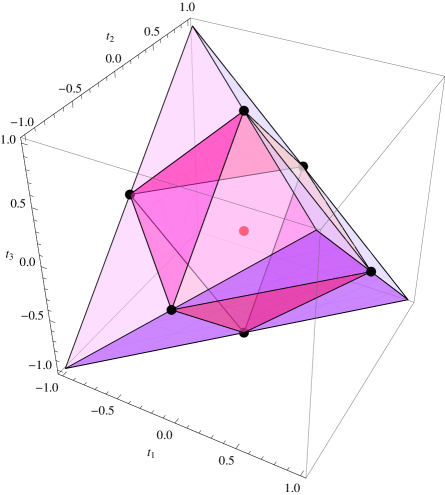
Figure 1. Geometry of Bell-diagonal states.

Acknowledgements.

SW thanks Thomas Kahle for a helpful correspondence about factorization of probability distributions. SW was partially supported by the DFG projects “Geometry and Complexity in Information Theory” and “Quantum Statistics: Decision problems and entropic functionals on state spaces”. MJZ is supported by the NSF of China under Grant No. 11401032 and SRF for ROCS, SEM.

Stephan Weis

e-mail: maths@stephan-weis.info

Max Planck Institute for

Mathematics in the Sciences

Inselstrasse 22

D-04103 Leipzig

Germany

Andreas Knauf

e-mail: knauf@math.fau.de

Department of Mathematics

Friedrich-Alexander-University

Erlangen-Nuremberg

Cauerstr. 11

D-91058 Erlangen

Germany

Nihat Ay
e-mail: nay@mis.mpg.de
Max Planck Institute for	Department of Mathematics	Santa Fe Institute
Mathematics in the Sciences	and Computer Science	1399 Hyde Park Road
Inselstrasse 22	Leipzig University	Santa Fe
D-04103 Leipzig	PF 10 09 20	New Mexico 87501
Germany	D-04009 Leipzig	USA
	Germany

Ming-Jing Zhao

e-mail: zhaomingjingde@126.com

Department of Mathematics

School of Science

Beijing Information Science and

Technology University

100192 Beijing

China

References

- [1] Amari, S.-I. (2001) Information geometry on hierarchy of probability distributions, IEEE Transactions on Information Theory 47(5) 1701–1711
- [2] Amari, S.-I., Nagaoka, H. (2000) Methods of Information Geometry, Translations of Mathematical Monographs 191, American Mathematical Soc., Oxford University Press
- [3] Aoki, S., Hara, H., Takemura, A. (2012) Markov Bases in Algebraic Statistics, Springer Series in Statistics 199, Springer, New York
- [4] Ay, N. (2001) Information geometry on complexity and stochastic interaction, MIS-Preprint: 95/2001
- [5] Ay, N. (2002) An information-geometric approach to a theory of pragmatic structuring, Annals of Probability 30(1) 416–436
- [6] Ay, N., Knauf, A. (2006) Maximizing multi-information, Kybernetika 42(5) 517–538
- [7] Ay, N., Olbrich, E., Bertschinger, N., Jost, J. (2011) A geometric approach to complexity, Chaos 21 037103
- [8] Bengtsson, I., Życzkowski, K. (2006) Geometry of Quantum States: An Introduction to Quantum Entanglement, Cambridge University Press
- [9] Benatti, F., Hudetz, T., Knauf, A. (1998) Quantum chaos and dynamical entropy, Communications in Mathematical Physics 198(3) 607–688
- [10] I. Bjelaković, J.-D. Deuschel, T. Krüger, R. Seiler, R. Siegmund-Schultze, A. Szkoła (2005) A Quantum Version of Sanov’s Theorem, Commun. Math. Phys. 260 659–671
- [11] Cafaro, C., Giffin, A., Lupo, C., Mancini, S. (2012) Softening the complexity of entropic motion on curved statistical manifolds, Open Systems & Information Dynamics 19(1) 1250001
-
[12]
Chen, J., Ji, Z., Li, C.-K., Poon, Y.-T., Shen, Y.,
Yu, N., Zeng, B., Zhou, D. (2014)
Principle of maximum entropy and quantum phase transitions,
arXiv:1406.5046[quant-ph] - [13] Coffman, V., Kundu, J., Wootters, W. K. (2000) Distributed entanglement, Physical Review A 61(5) 052306
- [14] Csiszár, I. (1967) On topological properties of f-divergences, Studia Sci. Math. Hungar. 2 329–339
- [15] Csiszár, I., Matúš, F. (2003) Information projections revisited, IEEE Transactions on Information Theory 49(6) 1474–1490
- [16] Csiszár, I., Matúš, F. (2008) Generalized maximum likelihood estimates for exponential families, Probab. Theory and Relat. Fields 141(1–2) 213–246
- [17] Cubitt, T., Montanaro, A. (2014) Complexity classification of local Hamiltonian problems, arXiv:1311.3161 [quant-ph]
- [18] Develin, M., Sullivant, S. (2003) Markov bases of binary graph models, Annals of Combinatorics 7(4) 441–466
- [19] Geiger, D., Meek, C., Sturmfels, B. (2006) On the toric algebra of graphical models, The Annals of Statistics 34(3) 1463–1492
- [20] Groisman, B., Popescu, S., Winter, A. (2005) Quantum, classical, and total amount of correlations in a quantum state, Physical Review A 72(3) 032317
- [21] Harremoës, P. (2007) Information topologies with applications, In Entropy, Search, Complexity (pp. 113–150), Springer Berlin Heidelberg
- [22] Horodecki, R., Horodecki, M. (1996) Information-theoretic aspects of inseparability of mixed states, Physical Review A 54(3) 1838–1843
- [23] Horodecki, R., Horodecki, P., Horodecki, M., Horodecki, K. (2009) Quantum entanglement, Reviews of Modern Physics 81(2) 865–942
- [24] Jaynes, E. T. (1957) Information theory and statistical mechanics. I./II., Physical Review 106(4) 620–630 and 108(2) 171–190
- [25] Kahle, T. (2010) Neighborliness of marginal polytopes, Contributions to Algebra and Geometry 51(1) 45–56
- [26] Kahle, T., Olbrich, E., Jost, J., Ay, N. (2009) Complexity measures from interaction structures, Physical Review E 79(2) 026201
- [27] Kay, A. (2012) Using separable Bell-diagonal states to distribute entanglement, Physical Review Letters 109(8) 080503
- [28] Kempe, J., Kitaev, A., Regev, O. (2006) The complexity of the local Hamiltonian problem, SIAM Journal on Computing 35(5) 1070–1097
- [29] Lang, M. D., Caves, C. M. (2010) Quantum discord and the geometry of Bell-diagonal states, Physical Review Letters 105(15) 150501
- [30] Lauritzen, S. L. (1996) Graphical Models, Oxford University Press
- [31] Linden, N., Popescu, S., Wootters, W. (2002) Almost every pure state of three qubits is completely determined by its two-particle reduced density matrices, Phys Rev Lett 89(20) 207901
- [32] Matúš, F. (2007) Optimality conditions for maximizers of the information divergence from an exponential family, Kybernetika 43 731–746
- [33] Modi, K., Paterek, T., Son, W., Vedral, V., Williamson, M. (2010) Unified view of quantum and classical correlations, Physical Review Letters 104(8) 080501
- [34] Niekamp, S., Galla, T., Kleinmann, M., Gühne, O. (2013) Computing complexity measures for quantum states based on exponential families, Journal of Physics A: Mathematical and Theoretical 46(12) 125301
- [35] Nielsen, M. A., Chuang, I. L. (2010) Quantum Computation and Quantum Information, Cambridge University Press
- [36] Nielsen, M. A., Kempe, J. (2001) Separable states are more disordered globally than locally, Physical Review Letters 86(22) 5184–5187
- [37] Ollivier, H., Zurek, W. H. (2001) Quantum discord: A measure of the quantumness of correlations, Physical Review Letters 88(1) 017901
- [38] Pachos, J. K. (2012) Introduction to Topological Quantum Computation, Cambridge University Press
- [39] Petz, D. (1994) Geometry of canonical correlation on the state space of a quantum system, Journal of Mathematical Physics 35(2) 780–795
- [40] Petz, D. (2008) Quantum Information Theory and Quantum Statistics, Springer
- [41] Rauh, J. (2011) Finding the maximizers of the information divergence from an exponential family, IEEE Trans. Inf. Theory 57(6) 3236–3247
- [42] Rockafellar, R. T. (1972) Convex Analysis, Princeton University Press
- [43] Rodman, L., Spitkovsky, I. M., Szkoła, A., Weis, S. (in preparation) Continuity of the maximum-entropy inference and numerical ranges
- [44] Rudolph, O. (2004) On extremal quantum states of composite systems with fixed marginals, Journal of Mathematical Physics 45(11) 4035–4041
- [45] Ruelle, D. (1999) Statistical Mechanics: Rigorous Results, World Scientific
- [46] Sachdev, S. (2014) Quantum Phase Transitions, Cambridge University Press, 2nd Edition
- [47] Shirokov, M. (2006) Entropy characteristics of subsets of states. I., Izvestiya: Mathematics 70(6) 1265–1292
- [48] Vedral, V., Plenio, M. B., Rippin, M. A., Knight, P. L. (1997) Quantifying entanglement, Physical Review Letters 78(12) 2275–2279
- [49] Wehrl, A. (1978) General properties of entropy, Rev Modern Phys 50(2) 221–260
- [50] Weis, S. (2011) Quantum convex support, Linear Algebra and its Applications 435(12) 3168–3188; (2012) Correction, ibid., 436(1), xvi
- [51] Weis, S. (2014) Information topologies on non-commutative state spaces, Journal of Convex Analysis 21(2) 339–399
- [52] Weis, S. (2015) The MaxEnt extension of a quantum Gibbs family, convex geometry and geodesics, AIP Conference Proceedings 1641 173-180
- [53] Weis, S., Knauf, A. (2012) Entropy distance: New quantum phenomena, Journal of Mathematical Physics 53(10) 102206
- [54] Wen, X.-G. (2004) Quantum Field Theory of Many-Body Systems, Oxford University Press
- [55] Zhou, D. L. (2008) Irreducible multiparty correlations in quantum states without maximal rank, Physical Review Letters 101 180505
- [56] Zhou, D. L. (2009) Irreducible multiparty correlations can be created by local operations, Physical Review A 80 022113