Dilaton gravity, charged dust, and (quasi-) black holes

Abstract

We consider Einstein-Maxwell-dilaton gravity with charged dust and interaction of the form $P(\chi)F_{\mu\nu}F^{\mu\nu}$, where $P(\chi)$ is an arbitrary function of the dilaton field $\chi$ that can be normal or phantom. For any regular $P(\chi)$, static configurations are possible with arbitrary functions $g_{00}=\exp(2\gamma(x^{i}))$ ($i=1,2,3$) and $\chi=\chi(\gamma)$, without any assumption of spatial symmetry. The classical Majumdar-Papapetrou system is restored by putting $\chi={\rm const}$. Among possible solutions are black-hole (BH) and quasi-black-hole (QBH) ones. Some general results on BH and QBH properties are deduced and confirmed by examples. It is found, in particular, that asymptotically flat BHs and QBHs can exist with positive energy densities of matter and both scalar and electromagnetic fields.

An important type of static charged dust configurations is represented by the Majumdar-Papapetrou (MP) solution majumdar ; papa ; it comprises an equilibrium between gravitational attraction and electric repulsion without any spatial symmetry assumption: equilibrium is established for any spatial shape of the charged dust cloud provided the charge to mass density ratio takes everywhere the proper value, $\rho_{e}/\rho_{m}=\pm 1$ in natural units ($c=G=1$),

The MP system was recently revived in a new context, that of the so-called quasi-black holes (QBHs) lemos1 –mein11 . Using the fact that in this solution the force balance implies a charge-to-mass ratio similar to that in the vacuum extremal Reissner-Nordstrom solution, a configuration has been proposed where such a starlike object has a size very close to the horizon radius. Such a system looks, for a distant external observer, quite similar to a true BH, though an event horizon has not been formed.

We here extend this treatment to include a dilatonic scalar field, which can be partly motivated by studies in string theory. Along with general observations on possible equilibrium configurations [to be called dilatonic MP (DMP) systems), we consider BHs and QBHs supported by certain electric and scalar charge distributions. In particular, we try to find phantom-free configurations, i.e., those able to exist with positive-definite energy densities of matter and both fields.

This problem has been considered in a PhD thesis of one of the co-authors of this paper, Robson Silveira, who died in 2009 before completing his study. He obtained some initial results indicating that such scalar QBHs are really possible and described some of their main properties. Our goal here is to briefly report on a more general analysis strongly developing his findings. A more detailed presentation can be found in Ref. we-13 .

Consider the Lagrangian ($c=G=1$)

$$L=\frac{1}{16\pi}\Big{[}R+2\varepsilon(\partial\chi)^{2}-F^{2}P(\chi)\Big{]}+L_{m}+A_{\mu}j^{\mu}+J\chi,$$ (1)

where $\varepsilon=\pm 1$ ($\varepsilon=1$ for a normal scalar field $\chi$), $L_{m}$ is the Lagrangian of matter, $J$ is the scalar charge density, $F^{2}\equiv F^{\alpha\beta}F_{\alpha\beta}$ ($F_{\mu\nu}=\partial_{\mu}A_{\nu}-\partial_{\nu}A_{\mu}$, the electromagnetic field), $j^{\mu}=\rho_{e}u^{\mu}$ is the 4-current, and $u^{\mu}$ is the 4-velocity. We do not fix the sign of $P(\chi)$ to provide correspondence with clem1 ; clem2 . Following the ideas of the MP solution, we consider a static equilibrium with the metric

$$ds^{2}={\,\rm e}^{2\gamma}dt^{2}-{\,\rm e}^{-2\gamma}h_{ik}dx^{i}dx^{k},$$ (2)

and assume only the electric components $F_{0i}=-F_{i0}=\phi_{i}$ to be nonzero among $F_{\mu\nu}$; $\gamma$, $h_{ik}$, $\phi$, $\chi$ are functions of $x^{i}$, $i=1,2,3$; $h_{ik}$ is the Euclidean flat metric, in general, in curvilinear coordinates. We use the notations $\gamma_{i}=\partial_{i}\gamma$, $\phi_{i}=\partial_{i}\phi$ etc; spatial indices are raised and lowered with the metric $h_{ik}$ and its inverse $h^{ik}$. Also, $u^{\mu}=\delta^{\mu}_{0}{\,\rm e}^{-\gamma}$.

The equations for $\chi$ and $\phi$ and the relevant combinations of the Einstein equations can be written in the following form:

$$2\varepsilon{\,\rm e}^{2\gamma}\Delta\chi+P_{\chi}\phi_{i}\phi^{i} = -8\pi J,$$ (3)

$${}\nabla_{i}\left({\,\rm e}^{-2\gamma}P\phi^{i}\right) = 4\pi\rho_{e}{\,\rm e}^{-3\gamma},$$ (4)

$${}{\,\rm e}^{2\gamma}(\gamma_{i}\gamma^{k}+\varepsilon\chi_{i}\chi^{k}) = P\,\phi_{i}\phi^{k},$$ (5)

$${}{\,\rm e}^{2\gamma}(\Delta\gamma-\gamma^{i}\gamma_{i}-\varepsilon\chi^{i}\chi_{i}) = 4\pi\rho_{m},$$ (6)

where $\nabla_{i}$ and the Laplace operator $\Delta=\nabla_{i}\nabla^{i}$ are defined in terms of the metric $h_{ik}$. Eq. (5) does not contain the densities, hence it holds both in vacuum and in matter; Eq. (6) is a convenient expression for $\rho_{m}$ in terms of $\gamma(x)$ and $\chi(x)$. The Einstein equations also lead to the equilibrium condition

$$\rho_{m}\gamma_{i}-\rho_{e}\phi_{i}{\,\rm e}^{-\gamma}=J\chi_{i}.$$ (7)

The tensor equation (5) implies that $\gamma$, $\chi$ and $\phi$ are functionally related, and if $\gamma\neq{\rm const}$, we can put $\phi=\phi(\gamma)$, $\chi=\chi(\gamma)$; Eq. (5) then reduces to

$${\,\rm e}^{2\gamma}(1+\varepsilon\chi_{\gamma}^{2})=P\phi_{\gamma}^{2}.$$ (8)

Hence we have the following arbitrariness: for any $P(\chi)$ and any 3D profile $\gamma(x^{i})$, even more than that, for an arbitrary scalar field distribution $\chi=\chi(\gamma)$, we find $\phi(\gamma)$ from (5), and the remaining field equations (3), (4) and (6) give us the mass, electric and scalar charge distributions that support this field configuration.

In what follows we will try to obtain examples of BH and QBH configurations in the simplest case of spherical symmetry, and of special interest can be those where all kinds of matter are “normal”, i.e., $P>0$, $\varepsilon=+1$ and $\rho_{m}\geq 0$.

The classical MP system is reproduced if we put $\chi={\rm const}$, $P(\chi)\equiv 1$, and we necessarily obtain $|\rho_{e}|=\rho_{m}$. On the contrary, putting $\phi={\rm const}$, we obtain MP-like systems with an arbitrary function $\gamma(x^{i})$, existing only with a phantom $\chi$ field, as follows from Eq. (8).

In the case of spherical symmetry, the metric (2) reads

$$ds^{2}={\,\rm e}^{2\gamma}dt^{2}-{\,\rm e}^{-2\gamma}(dx^{2}+x^{2}d\Omega^{2}),$$ (9)

where $x$ is a radial coordinate and $d\Omega^{2}$ is the line element on a unit sphere. The usual spherical (areal) radius is $r(x)=x{\,\rm e}^{-\gamma}$. Our set of equations takes the form

$$2\varepsilon x^{-2}{\,\rm e}^{2\gamma}(x^{2}\chi^{\prime})^{\prime}+P_{\chi}\phi^{\prime}{}^{2} = -8\pi J(x),$$ (10)

$$x^{-2}\big{(}P{\,\rm e}^{-2\gamma}x^{2}\phi^{\prime}\big{)}^{\prime} = 4\pi\rho_{e}{\,\rm e}^{-3\gamma},$$ (11)

$${\,\rm e}^{2\gamma}(\gamma^{\prime\prime}+2\gamma^{\prime}/x-\gamma^{\prime}{}^{2}-\varepsilon\chi^{\prime}{}^{2}) = 4\pi\rho_{m},$$ (12)

$$\gamma^{\prime}{}^{2}+\varepsilon\chi^{\prime}{}^{2} = {\,\rm e}^{-2\gamma}P\phi^{\prime}{}^{2},$$ (13)

$$\rho_{m}\gamma^{\prime}-\rho_{e}\phi^{\prime}{\,\rm e}^{-\gamma} = J\chi^{\prime},$$ (14)

where the prime denotes $d/dx$. The above arbitrariness transforms here into the freedom of choosing the functions $\gamma(x)$ and $\chi(x)$ even if the coupling function $P(\chi)$ has been prescribed from the outset. All other quantities are then found from Eqs. (10)–(14).

It is of interest how to choose the arbitrary functions in order to obtain a starlike configuration with a regular center or a BH. It is also of interest to seek phantom-free configurations such that $\varepsilon=+1$ and $\rho_{m}\geq 0$.

A regular center is obtained in the metric (9) at $x=0$ if and only if $\gamma(x)=\gamma_{c}+O(x^{2}),\ \gamma_{c}={\rm const}$. Using a Taylor expansion for ${\,\rm e}^{2\gamma}\equiv A(x)$ at small $x$, one can show that $\rho_{m}>0$ near the center requires that $g_{00}=A(x)$ should have there a minimum.

Near a horizon we must have ${\,\rm e}^{2\gamma}\sim(x-x_{\rm hor})^{n}$, where $n\in{\mathbb{N}}$ is the order of the horizon. From (9) it is clear that a horizon of finite radius $r_{\rm hor}=x{\,\rm e}^{-\gamma}\big{|}_{x=x_{\rm hor}}$ is only possible with $x_{\rm hor}=0$ and $n=2$ (a double, or extremal horizon). Thus at small $x$ we can write $A(x)={{\textstyle\frac{1}{2}}}A_{2}x^{2}+{\textstyle\frac{1}{6}}A_{3}x^{3}+\cdots$, $A_{i}={\rm const},\ A_{2}>0$. Assuming that $\chi$ and $\chi^{\prime}$ are finite at the horizon, we obtain $\rho_{m}\sim x^{2}$, but it can be of any sign without a direct correlation with $\varepsilon$. From the field equations it follows that $\rho_{e}\sim x$ or possibly $\rho_{e}=o(x)$, while $J$ generically tends there to a finite limit. Thus such configurations, being in general perfectly regular and smooth, still contain an anomaly: the density ratios $\rho_{e}/\rho_{m}$ and $J/\rho_{m}$ are infinite at the horizon.

For dust balls of finite size placed in vacuum, the external domain is described by the corresponding “vacuum” Einstein-Maxweel-dilaton (EMD) solution; however, such solutions to the field equations are only known for some special choices of $P(\chi)$, e.g., $P={\,\rm e}^{2\lambda\chi}$ BSh-77 ; dbh1 ; dbh2 . Therefore, instead, we consider asymptotically flat matter distributions with a smoothly decaying density. At large $x$ we can take

$$A(x)=1-\frac{2m}{x}+\frac{q_{*}^{2}}{x^{2}}+\cdots,\ \ \ \chi(x)=\chi_{\infty}+\frac{\chi_{1}}{x}+\cdots,$$ (15)

and Eq. (12) then yields

$$4\pi\rho_{m}=\frac{1}{x^{4}}(-3m^{2}+q_{*}^{2}-\varepsilon\chi_{1}^{2})+o(x^{-4}).$$ (16)

This clearly shows that large charges $q$ are necessary for obtaining $\rho_{m}>0$ if $\varepsilon=+1$. (Note that the extreme Reissner-Nordström solution with the charge $q=m$ corresponds in the notation (15) to $q_{*}^{2}=3m^{2}$.) The densities $\rho_{e}$ and $J$ also behave in general as $1/x^{4}$ at large $x$.

Integral charges. The field at flat spatial infinity is characterized by integral charges: the electric charge $q$ such that the electric field strength is $\phi^{\prime}=q/x^{2}+o(1/x^{2})$, the scalar charge $D$ such that $\chi^{\prime}=D/x^{2}+o(1/x^{2})$, and the mass $m$ corresponding to the Schwarzschild asymptotic ${\,\rm e}^{\gamma}\approx 1-m/x$, hence $\gamma^{\prime}\approx m/x^{2}$ (note that $x\approx r$ at large $x$). A relation between these three quantities directly follows from Eq. (13). Indeed, multiply (13) by $x^{4}$ and take the limit $x\to\infty$ to obtain

$$m^{2}-q^{2}+\varepsilon D^{2}=0,$$ (17)

since ${\,\rm e}^{\gamma}\to 1$ and $P\to 1$ (assuming that a weak electromagnetic field should be Maxwell). This generalizes a similar relation (2.12) from clem2 , written there for vacuum EMD systems with $P(\chi)\sim{\,\rm e}^{2\lambda\chi}$.

Thus, as compared to the MP system where $q=\pm m$, a balance in the DMP system requires $m^{2}>q^{2}$ if $\varepsilon=-1$ (both electric and phantom scalar fields are repulsive), but $m^{2}<q^{2}$ with a canonical, attractive scalar field.

Eq. (17) is valid for all asymptotically flat  (islandlike) EMD systems since they are approximately spherically symmetric in the asymptotic region.

Quasi-black holes. By definition, in some region $r\leq r^{*}(c)$ of a QBH it holds that ${\,\rm e}^{\gamma}\sim c$, where $c$ is a small parameter, and the limit $c\to 0$ usually corresponds to a BH. The most general static, spherically symmetric QBH in our problem setting is a system with the metric (9) and a regular center, and at small $x$ we can write

$${\,\rm e}^{2\gamma}\equiv A(x,c)=A_{0}(c)+{{\textstyle\frac{1}{2}}}A_{2}(c)x^{2}+\cdots,$$ (18)

where $A_{0}(c)\to 0$ as $c\to 0$ while $A_{2}(0)$ is finite. Without loss of generality we can assume

$${\,\rm e}^{2\gamma}=\frac{x^{2}+c^{2}}{f^{2}(x,c)},$$ (19)

where $f$ is a smooth function that has a well-defined nonzero limit $c\to 0$. The value $c=0$ in (19) corresponds to an extreme BH metric with a horizon at $x=0$. In particular, taking $f(x,0)=x+m$, we obtain the extreme Reissner-Nordström metric. At small enough $c$ and $x\lesssim c$, $e^{2\gamma}=O(c^{2})$ is arbitrarily small.

Let us stress that, given (19), the region where the “redshift function” ${\,\rm e}^{\gamma}$ is small, is itself not small at all. Indeed, suppose $f(x,c)=O(1)$, and $c\ll 1$. Then the radius $r(c)$ of the sphere $x=c$ (which belongs to the high redshift region) is $f(c,c)/\sqrt{2}=O(1)$; the distance from the center to this sphere, $\int_{0}^{c}{\,\rm e}^{-\gamma}\,dx$, is also $O(1)$.

Example 1. Let us choose the metric function

$${\,\rm e}^{\gamma}=\frac{z}{m+2z-y},\ \ y:=\sqrt{x^{2}+a^{2}},\ \ z:=\sqrt{x^{2}+c^{2}},$$ (20)

with certain positive constants $m,\ a,\ c$. At small and large $x$ we have

$$x\to 0: {\,\rm e}^{2\gamma}=\frac{c^{2}}{(m{-}a{+}2c)^{2}}+x^{2}\,\frac{m{-}a{+}c^{2}/a}{(m{-}a{+}2c)^{3}}$$ (21)

$${}\hskip 72.26999pt+O(x^{4}),$$

$${}x\to\infty: {\,\rm e}^{2\gamma}=1-\frac{2m}{x}+\frac{3m^{2}{+}a^{2}{-}c^{2}}{x^{2}}+O(x^{-3}).$$ (22)

The system has a regular center and is asymptotically flat, and $m$ is the Schwarzschild mass. Assuming

$$c<a<m,$$ (23)

we can be sure that $\rho_{m}>0$ near the center since ${\,\rm e}^{\gamma}$ has a minimum there (see above). For $\rho_{m}$ there is a bulky expression leading to $\rho_{m}>0$ for proper choices of the dilaton field profile $\chi(x)$ with $\varepsilon=+1$ under the condition (23). It is the case, for instance, if we assume

$$\chi^{\prime}=b/y^{2},\hskip 28.45274ptb={\rm const}>0$$ (24)

with sufficiently small $b$.

The expressions for the electric and scalar charge densities are bulky, but their particular form can add nothing to our understanding of the situation; it is only important that they are finite and regular.

The limit $c\to 0$ leads to an extreme BH metric,

$${\,\rm e}^{\gamma}=\frac{x}{m+2x-y},\hskip 28.45274pty:=\sqrt{x^{2}+a^{2}}.$$ (25)

We thus obtain an asymptotically flat BH without phantoms. With (24) for $\chi$ and $\varepsilon=+1$, we obtain from (25)

$$4\pi\rho_{m}=\frac{x^{2}[(a^{2}+b^{2})y-b^{2}(2x+m)]}{y^{4}(2x-y+m)^{3}}.$$ (26)

We have $\rho_{m}>0$ at all $x>0$ in a certain region of the parameter space. Thus, putting $m=1$ (fixing the units) and $a=0.5$ (for example), we find that $\rho_{m}>0$ for $0<b<b_{0}\approx 0.369$.

The expressions for $\rho_{e}$ and $J$ are cumbersome; it is only important that, for a generic choice of $P(\chi)$, they are everywhere finite and regular and behave at the horizon as described above.

Example 2. Our framework allows for describing polycentric systems, with any number of mass concentrations. For instance, one can consider the metric (2) in Cartesian coordinates $x^{i}=(x,y,z)$ (so that $h_{ik}=\delta_{ik}$) and choose

$${\,\rm e}^{-\gamma(x^{i})}\equiv f(x^{i})=\frac{1}{n}\sum_{a=1}^{n}f_{a}(X_{a}),$$ (27)

where $f_{a}$ are functions of $X_{a}:=|x^{i}-x^{i}_{a}|$, $x^{i}_{a}$ being the (fixed) coordinates of the $a$-th center. As $f_{a}$, one can take any functions providing asymptotically flat spherically symmetric solutions, e.g., BHs or QBHs. A complete solution is obtained after choosing the function $\chi(\gamma)$, or equivalently $\chi(f)$, which should be regular at all relevant values of $f$ and decay sufficiently rapidly at spatial infinity, as $f\to 1$.

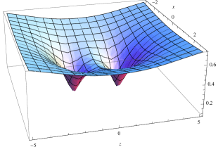
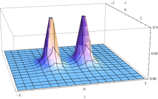
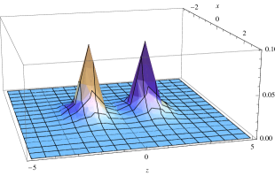
Figure 1: Plots for Example 2, sections $y=0$ of different 3D profiles for a system of two identical QBHs. Left: the metric function ${\,\rm e}^{2\gamma(x,y,z)}$ for $m_{1}=m_{2}=1$, $a=1.5$, $c_{1}=c_{2}=0.2$. Middle: the density $\rho_{m}(x,y,z)$ for the same parameters and $b=0$, i.e., for a pure MP system. Right: the same for $\varepsilon=+1$ and $b=0.07$, i.e., for a DMP system with the specified $\chi(f)$.

What follows is an example of a system of two QBHs: let

$${}f(x^{i})=\frac{m_{1}+z_{1}}{2z_{1}}+\frac{m_{2}+z_{2}}{2z_{2}},$$ (28)

$${}\chi(f)={{\displaystyle\frac{1}{2}}}b(f-1)^{2},$$ (29)

$${}z_{1}:=\big{(}|\vec{x}-\vec{x}_{1}|^{2}+c_{1}^{2}\big{)}^{1/2},\ \ \ z_{2}:=\big{(}|\vec{x}-\vec{x}_{2}|^{2}+c_{2}^{2}\big{)}^{1/2},$$

$${}\vec{x}_{1}=(0,\ 0,\ a),\ \ \ \ \vec{x}_{2}=(0,\ 0,\ -a),$$

with constants $m_{1}>0,\ m_{2}>0,\ a>0,\ b\geq 0$, $c_{1}\geq 0$ and $c_{2}\geq 0$. The electric potential $\phi$ and all densities are found from Eqs. (8), (3), (4), and (6). In particular, for the mass density we obtain

$${}4\pi\rho_{m}=\frac{1}{f^{2}(x^{i})}\biggl{[}\frac{3m_{1}c_{1}^{2}}{z_{1}^{2}(m_{1}+z_{1})^{3}}$$

$${}\hskip 28.45274pt+\frac{3m_{2}c_{1}2^{2}}{z_{2}^{2}(m_{2}+z_{2})^{3}}-\varepsilon b^{2}(f-1)^{2}f^{i}f_{i}\biggr{]}.$$ (30)

The special case $b=0$ corresponds to a bicentric MP configuration. If $c_{1}$ or $c_{2}$ is zero, the corresponding “center” is a BH, while at small nonzero $c_{a}$ it is a QBH.

Figure 1 shows the 3D behavior of the metric function $e^{2\gamma}\equiv f^{-2}(x^{i})$ and the mass density $\rho_{m}(x^{i})$ for the chosen example of a system of two QBHs for the specified parameter values. Evidently, the density is everywhere positive in both cases in Fig. 1 [middle (a MP system) and right (a DMP system with a canonical scalar field)], although inclusion of a scalar field makes it smaller.

In conclusion, let us enumerate the main results.

1. It has been shown that, with the Lagrangian (1), static configurations are possible with arbitrary functions $g_{00}={\,\rm e}^{2\gamma(x^{i})}$ ($i=1,2,3$) and $\chi=\chi(\gamma)$, for any regular coupling function $P(\chi)$, without any assumption of spatial symmetry.

2. There are purely scalar analogs of MP systems, but only with phantom scalar fields.

3. There is a universal balance condition, (17), between the Schwarzschild mass and the electric and scalar charges, valid for any asymptotically flat DMP systems, including those with horizons and/or singularities. It generalizes the results previously obtained for special cases (e.g., clem2 ).

4. In the case of spherical symmetry, the existence conditions have been formulated for BH and QBH configurations with smooth matter, electric charge and scalar charge density distributions. It turns out that horizons in DMP systems are second-order (extremal), in agreement with the general properties of QBHs lemos4 .

5. Examples of phantom-free spherically symmetric BH and QBH solutions have been obtained, and an example of a phantom-free system of two QBHs.

References

(1)
S.D. Majumdar, Phys. Rev. 72, 390 (1947).
(2)
A. Papapetrou, Proc. Roy. Irish Acad. A51, 191 (1947).
(3)
J.P.S. Lemos and E.J. Weinberg, Phys. Rev. D 69, 104004
(2004).
(4)
J.P.S. Lemos and O.B. Zaslavskii, Phys. Rev. D 76,
084030 (2007).
(5)
J.P.S. Lemos and O.B. Zaslavskii, Phys. Rev. D 82,
024029 (2010).
(6)
José P.S. Lemos and O.B. Zaslavskii, Phys. Lett. B 695, 37
(2011).
(7)
Jose P.S. Lemos and V.T. Zanchin
Phys. Rev. D 81, 124016 (2010); arXiv: 1004.3574
(8)
José P.S. Lemos,
Sci. Proc. Kazan University
(Uchonye Zapiski Kazanskogo Universiteta
(UZKGU)) 153, 215 (2011); arXiv: 1112.5763.
(9)
R. Meinel and M. Hütten,
Class. Quantum Grav. 28, 225010 (2011).
(10)
K.A. Bronnikov, J.C. Fabris, R. Silveira, and O.B. Zaslavskii,
arXiv: 1312.4891.
(11)
G. Clément, J.C. Fabris, and M.E. Rodrigues,
Phys. Rev. D 79, 064021 (2009).
(12)
M. Azreg-Ainou, G. Clément, J.C. Fabris, and M.E. Rodrigues,
Phys. Rev. D 83, 124001 (2011); arXiv: 1102.4093.
(13)
K.A. Bronnikov and G.N. Shikin,
Izv. Vuzov SSSR, Fiz., No. 9, 25 (1977);
Russ. Phys. J. 20, 1138 (1977).
(14)
G. W. Gibbons and K. Maeda, Nucl. Phys. B 298, 741 (1988).
(15)
D. Garfinkle, G.T. Horowitz, and A. Strominger,
Phys. Rev. D 43, 3140 (1991);
45, 3888(E) (1992).