A self-interaction-free local hybrid functional: accurate binding energies
vis-à-vis accurate ionization potentials from Kohn-Sham eigenvalues

Abstract

We present and test a new approximation for the exchange-correlation (xc) energy of Kohn-Sham density functional theory. It combines exact exchange with a compatible non-local correlation functional. The functional is by construction free of one-electron self-interaction, respects constraints derived from uniform coordinate scaling, and has the correct asymptotic behavior of the xc energy density. It contains one parameter that is not determined ab initio. We investigate whether it is possible to construct a functional that yields accurate binding energies and affords other advantages, specifically Kohn-Sham eigenvalues that reliably reflect ionization potentials. Tests for a set of atoms and small molecules show that within our local-hybrid form accurate binding energies can be achieved by proper optimization of the free parameter in our functional, along with an improvement in dissociation energy curves and in Kohn-Sham eigenvalues. However, the correspondence of the latter to experimental ionization potentials is not yet satisfactory, and if we choose to optimize their prediction, a rather different value of the functional’s parameter is obtained. We put this finding in a larger context by discussing similar observations for other functionals and possible directions for further functional development that our findings suggest.

I Introduction

Kohn-Sham (KS) density-functional theory (DFT)Hohenberg and Kohn (1964); Kohn and Sham (1965) has become one of the most frequently used theories for electronic structure calculations. It employs the electron ground-state density, $n(\mathbf{r})$, as the central quantity and accounts for all electronic interaction beyond the classical electrostatic (Hartree) repulsion, $E_{\mathrm{H}}$, via the exchange-correlation (xc) energy functional, $E_{\mathrm{xc}}[n]$ Parr and Yang (1989); Dreizler and Gross (1995); Fiolhais et al. (2003). Even though the xc energy is typically the smallest component in the ground-state total energy, it governs binding properties, geometrical structures, and ionization processes Kurth and Perdew (2000); Burke (2012); Fiolhais et al. (2003). Thus, the quality of a DFT calculation depends decisively on the functional approximation put to task.

It has become popular to categorize density functional approximations according to the “Jacob’s ladder” scheme introduced in Ref. Perdew and Schmidt (2001). Typically, the accuracy of a density functional approximation (DFA) improves when more “ingredients” are allowed in the functional construction, at the price of increased complexity. The local spin-density approximation (LDA) Kohn and Sham (1965), which approximates $E_{xc}[n]$ based on the xc energy of the homogeneous electron gas Ceperley and Alder (1980); Perdew and Wang (1992); Perdew and Zunger (1981); Vosko et al. (1980), and even more so the semi-local generalized gradient approximations (GGAs) Perdew and Wang (1986); Becke (1988); Lee et al. (1988); Perdew (1991); Perdew et al. (1996a); Wu and Cohen (2006); Haas et al. (2011), which additionally take the density gradient into account, offer a favorable ratio of computational expense and accuracy Burke (2012). Hybrid functionals Becke (1993a, b); Perdew et al. (1996b); Stephens et al. (1994); Adamo and Barone (1999); Ernzerhof and Scuseria (1999) typically reach yet greater accuracy by combining a fixed percentage of Fock exchange

$$E_{x}^{ex}=-\frac{1}{2}\sum_{\begin{subarray}{c}i,j=1\\ \sigma=\uparrow,\downarrow\end{subarray}}^{N_{\sigma}}\int\!\!\!\int\frac{\varphi_{i\sigma}^{*}(\mathbf{r})\varphi_{j\sigma}(\mathbf{r})\varphi_{i\sigma}(\mathbf{r}^{\prime})\varphi_{j\sigma}^{*}(\mathbf{r}^{\prime})}{|\mathbf{r}-\mathbf{r}^{\prime}|}\,\mathrm{d}^{3}r\mathrm{d}^{3}r^{\prime},$$ (1)

with (semi-)local exchange and correlation energy terms (Hartree atomic units are used throughout). Eq. (1) evaluated with the exact Kohn-Sham orbitals defines the exact Kohn-Sham exchange energy. Self-consistent Kohn-Sham calculations based on the energy of Eq. (1) use the optimized effective potential (OEP) equation (see Grabo et al. (1997); Engel and Dreizler (2011); Kümmel and Kronik (2008) and references therein). When we use the abbreviation EXX in the following, we always refer to this Kohn-Sham variant of exact exchange.

While the aforementioned functionals in many cases predict binding energies and bond-lengths reliably, semi-local DFAs and to some extent also hybrid functionals are less reliable for ionization processes, photoemission spectra and densities of states. Very early on it was realized that this problem is closely related to the (one-electron) self-interaction (SI) Perdew and Zunger (1981) error, i.e., to the fact that in exact DFT $E_{\mathrm{xc}}+E_{\mathrm{H}}$ should vanish for any one-electron system, but does not do so for these DFAs. Due to the SI error and the fact that semi-local functionals “average over” the derivative discontinuity Perdew and Levy (1983); Tozer and Handy (1998), the Kohn-Sham eigenvalues of the above mentioned approximate functionals typically fulfill neither the exact condition that the highest occupied eigenvalue $\varepsilon_{\mathrm{ho}}$ should match the first ionization potential (IP) Perdew et al. (1982); Levy et al. (1984); Almbladh and von Barth (1985); Perdew and Levy (1997), nor the approximate but for practical purposes equally important condition that upper valence eigenvalues are good approximations to higher IPs when they are calculated from accurate xc potentials Stowasser and Hoffmann (1999); Chong et al. (2002); Körzdörfer et al. (2009, 2010); Dauth et al. (2011); Bleiziffer et al. (2013).

Although the interpretation of occupied eigenvalues even with the exact xc potential is approximate (except for $\varepsilon_{\mathrm{ho}}$), it is of great practical importance. For example, the band-structure interpretation of Kohn-Sham eigenvalues has had a great impact on solid-state physics and materials science Cohen and Chelikowsky (1988). In recent years the interpretation of eigenvalues has become particularly important in the field of molecular semiconductors and organic electronics. Efforts to understand, e.g., photoemission experiments, have revealed severe shortcomings of traditional DFAs that go considerably beyond a spurious global shift of the eigenvalue spectrum Dori et al. (2006); Mundt et al. (2006); Mundt and Kümmel (2007); Körzdörfer et al. (2009, 2010); Körzdörfer and Kümmel (2010); Dauth et al. (2011); Marom et al. (2008); Marom and Kronik (2009); Marom et al. (2010); Bisti et al. (2011). A similar problem is witnessed also in solid state systems Rinke et al. (2005); Fuchs et al. (2007); Fuchs and Bechstedt (2008); Rödl et al. (2009); Betzinger et al. (2012, 2013). We emphasize that these problems of interpretation arise already for the occupied eigenvalues, i.e., the issues are separate from the well known band-gap problem Perdew and Levy (1983); Sham and Schlüter (1983); Kümmel and Kronik (2008); Kronik et al. (2012) of Kohn-Sham theory. The KS EXX potential leads to band structures and eigenvalues that match experiments much better than the eigenvalues from (semi-)local approximations Bylander and Kleinman (1995, 1996); Grabo et al. (1997); Städele et al. (1999); Mundt et al. (2006); Engel and Schmid (2009).

A comparison to hybrid functionals is more involved, because already the occupied eigenvalue spectrum depends sensitively on whether one uses the hybrid functional in a KS or a generalized KS calculation Körzdörfer and Kümmel (2010). For well understood reasons Perdew and Levy (1983); Sham and Schlüter (1983), the differences between the KS and the generalized KS eigenvalues become yet larger for unoccupied eigenvalues (see, e.g., the review Kronik et al. (2012)).This article’s focus is on Kohn-Sham theory, therefore we do not discuss the comparison to hybrid functionals used in the generalized KS scheme in detail. We note, however, that in particular range-separated hybrid functionals used in the generalized KS approach can predict gaps and band structures quite accurately, as discussed, e.g., in Henderson et al. (2011); Kronik et al. (2012), but global hybrid functionals tend to yield a less reliable density of states for complex systems than self-interaction free Kohn-Sham potentials Körzdörfer and Kümmel (2010); Dauth et al. (2011).

Besides these practical benefits, EXX also appears as a natural component of DFAs because it may be considered attractive to treat as many energy components as possible exactly, and including EXX has shown to be beneficial for, e.g., describing ionization, dissociation and charge transfer processes  Kümmel and Kronik (2008). However, bare EXX is a very poor approximation for binding energies, (see, e.g., Refs. Engel et al. (2000),Engel and Dreizler (2011), and Fiolhais et al. (2003), chapter 2). Combining EXX with a (semi-)local correlation term in many situations leads to results of inferior quality compared to pure EXX or semi-local DFAs, because of an imbalance between the delocalized exchange hole and the localized correlation hole Gunnarsson and Lundqvist (1976); Perdew and Schmidt (2001); Prodan and Kohn (2005); Kümmel and Kronik (2008).

One promising approach for combining EXX with appropriate correlation in a balanced way is the local hybrid form Cruz et al. (1998); Jaramillo et al. (2003); Perdew et al. (2008)

$$e_{xc}(\mathbf{r})=(1-f[n](\mathbf{r}))e^{ex}_{x}(\mathbf{r})+f[n](\mathbf{r})e^{sl}_{x}(\mathbf{r})+e^{sl}_{c}(\mathbf{r}).$$ (2)

Here, $e_{xc}(\mathbf{r})$ is the xc energy density per particle that yields the xc energy via $E_{xc}[n]=\int n(\mathbf{r})\,e_{xc}(\mathbf{r})\,\mathrm{d}^{3}r$. The quantities $e^{sl}_{x}(\mathbf{r})$ and $e^{sl}_{c}(\mathbf{r})$ denote exchange and correlation energy densities per particle, respectively, approximated with (semi-)local expressions, whereas $e^{ex}_{x}(\mathbf{r})$ represents the EXX energy density per particle deduced from Eq. (1). The function $f[n](\mathbf{r})$ is the local mixing function (LMF). It is a functional of the density and a decisive part of the local hybrid concept.

Eq. (2) can be viewed as a generalization of the common (global) hybrids. Instead of a fixed amount of EXX, the local hybrid can describe different spatial regions of a system with varying combinations of EXX and semi-local xc, by means of $f[n](\mathbf{r})$ (where $0\leq f\leq 1$). For example, whereas one-electron regions are supposed to be well-described using EXX, regions of slowly varying density are expected to be captured appropriately by (semi-)local xc functionals. The idea of local hybrids can also be understood in terms of the adiabatic connection theorem Ernzerhof et al. (1997), because $f[n](\mathbf{r})$ may offer further flexibility in an accurate construction of the coupling-constant-dependent xc energy Cruz et al. (1998), especially for small coupling constant values.

The local hybrid form was pioneered by Jaramillo et al. Jaramillo et al. (2003) with a focus on reducing the one-electron SI-error in single-orbital regions. Numerous further local hybrid constructions followed Arbuznikov et al. (2006); Arbuznikov and Kaupp (2007); Bahmann et al. (2007); Kaupp et al. (2007); Perdew et al. (2008); Arbuznikov et al. (2009); Haunschild et al. (2009); Haunschild and Scuseria (2010a, b); Theilacker et al. (2011). They proposed various LMFs with different one-electron-region indicators, suggested several (semi-)local exchange and correlation functionals to be used in the construction, and followed different procedures to satisfy known constraints and determine remaining free parameters.

In the present manuscript we propose a new local-hybrid approximation that combines full exact exchange with a compatible correlation functional. The development is guided by the philosophy of fulfilling known constraints Perdew et al. (2005): Our xc energy density per particle, $e_{xc}$, is one-electron SI-free, possesses the correct behaviour under uniform coordinate scaling, and has the right asymptotic behaviour at large distances. It includes one free parameter that is not determined uniquely from these constraints.

In difference to earlier work, our emphasis is not on improving further the accuracy of binding energies beyond the one that was achieved with global hybrids. Instead, we focus on whether it is possible to construct an approximation that yields binding energies of at least the same quality as established hybrids and at the same time affords other advantages, notably KS eigenvalues that approximate IPs reasonably well. We find that if we choose the parameter in our functional by optimizing the prediction of binding energies, the latter are obtained with an accuracy that is similar to the one reached with usual global hybrids. At the same time, we achieve a significant improvement in prediction of dissociation energy curves for selected systems. Improvement in prediction of the ionization energy via the highest occupied KS eigenvalue is also observed. It is especially large for alkali atoms. However, the quality of the ionization energy prediction is not yet satisfactory, and if we aim to optimize the prediction of the latter, a rather different value for the functional’s free parameter is obtained. We put this finding in a larger context by discussing similar observations for other functionals.

The paper is organized as follows: Section II is devoted to the description of the new local hybrid functional. Section III (and the Appendix) provide methodological and computational details. Sec. IV presents and discusses the results, and Sec. V offers conclusions and a summary.

II Construction of the functional

In the construction of our functional, we choose to concentrate on satisfying the following exact properties: (i) use the concept of full exact exchange, as defined by the correct uniform coordinate scaling Levy and Perdew (1985); Levy (1991) (see elaboration below); (ii) freedom from one-electron self-interaction Perdew and Zunger (1981); (iii) correct asymptotic behavior of the xc energy density per particle at $|\mathbf{r}|\rightarrow\infty$ van Leeuwen and Baerends (1994); (iv) reproduction of the homogeneous electron gas limit. In addition, we wish to maintain an overall balanced non-locality of exchange and correlation Perdew et al. (2008).

Regarding property (i), under the uniform coordinate scaling $\mathbf{r}\rightarrow\gamma\mathbf{r}$ the density transforms as $n_{\gamma}(\mathbf{r})=\gamma^{3}n(\gamma\mathbf{r})$, with its integral, $N$, unchanged and the exchange scales as $E_{x}[n_{\gamma}(\mathbf{r})]=\gamma E_{x}[n(\gamma\mathbf{r})]$ Fiolhais et al. (2003); Kümmel and Kronik (2008), which implies $e_{x}^{ex}[n_{\gamma}(\mathbf{r})]=\gamma e^{ex}_{x}[n(\gamma\mathbf{r})]$. This scaling relation is fulfilled, e.g., by $e_{x}^{L\!S\!D\!A}$, the exchange energy density per particle in the local spin-density approximation (LSDA).

For the correlation functional, $E_{c}[n]$, no such simple scaling rule exists: the correlation scales as $E_{c}[n_{\gamma}(\mathbf{r})]=\gamma^{2}E_{c}^{(1/\gamma)}[n(\mathbf{r})]$, where the superscript $(1/\gamma)$ indicates a system with an electron-electron interaction that is reduced by a factor of $\gamma$ Fiolhais et al. (2003). Additional scaling results for the correlation energy can be found in, e.g., Refs. Levy and Perdew (1985); Levy (1991). Here, we concentrate on the limiting case of high electron densities, i.e. $\gamma\rightarrow\infty$, where the xc energy should be dominated by $E_{x}[n]$, Levy (1991)

$$\lim_{\gamma\rightarrow\infty}\frac{E_{xc}[n_{\gamma}]}{E^{ex}_{x}[n_{\gamma}]}=1.$$ (3)

A functional is said to use full exact exchange if it obeys Eq. (3) Perdew et al. (2008).

With this definition in mind, we return to Eq. (2). Using $e_{xc}(\mathbf{r})=e^{ex}_{x}(\mathbf{r})+e_{c}(\mathbf{r})$, we obtain

$$e_{c}(\mathbf{r})=f[n](\mathbf{r})\left(e^{sl}_{x}(\mathbf{r})-e^{ex}_{x}(\mathbf{r})\right)+e^{sl}_{c}(\mathbf{r}).$$ (4)

We now see that when $f[n]$ scales in the high density limit as $\gamma^{a}$ with $a<0$, then it is clear that the first term on the RHS of Eq. (4) is a correlation contribution rather than an exchange term . Assuming $e^{sl}_{c}(\mathbf{r})$ scales as $\gamma^{b}$ with $b<1$, the functional $e_{xc}(\mathbf{r})$ that fulfills this condition can therefore justly be viewed as a combination of EXX, namely, $e^{ex}_{x}(\mathbf{r})$, and a compatible correlation term, $e_{c}(\mathbf{r})$.

The reduced density gradient Perdew et al. (1996a)

$$t^{2}(\mathbf{r}):=\left(\frac{\pi}{3}\right)^{1/3}\frac{a_{0}}{16\Phi^{2}(\zeta(\mathbf{r}))}\frac{|\nabla n(\mathbf{r})|^{2}}{n^{7/3}(\mathbf{r})},$$ (5)

where $a_{0}$ is the Bohr radius, $\Phi(\zeta(\mathbf{r}))=\frac{1}{2}\left((1+\zeta)^{2/3}+(1-\zeta)^{2/3}\right)$ and $\zeta(\mathbf{r})=(n_{\uparrow}(\mathbf{r})-n_{\downarrow}(\mathbf{r}))/(n_{\uparrow}(\mathbf{r})+n_{\downarrow}(\mathbf{r}))$ is the spin polarization, is a natural ingredient to be used to construct a $f[n](\mathbf{r})$ that aims at enforcing the uniform coordinate scaling, because in the high density limit $t^{2}\sim\gamma$. We make use of this quantity as described in detail below.

Property (ii) is reflected in the equation $E_{H}[n_{i\sigma}]+E_{xc}[n_{i\sigma}]=0$, where $n_{i\sigma}(\mathbf{r})=|\varphi_{i\sigma}(\mathbf{r})|^{2}$ are one-spin-orbital densities, with $\varphi_{i\sigma}(\mathbf{r})$ denoting the $i$-th KS-orbital in the spin-channel $\sigma$. One can attempt to realize such a one-spin-orbital condition by detecting regions of space in which the density is dominated by just one spin-orbital and making sure that full exact exchange and zero correlation is used there. Previous works have discussed the use of iso-orbital indicators Becke (1985); Dobson (1992); Perdew et al. (1999); Kümmel and Perdew (2003) for similar tasks. Here, we define a one-spin-orbital-region indicator by

$$d(\mathbf{r})=\frac{\tau_{W}(\mathbf{r})}{\tau(\mathbf{r})}\zeta^{2}(\mathbf{r}),$$ (6)

where $\tau_{W}(\mathbf{r})=|\nabla n(\mathbf{r})|^{2}/(8n(\mathbf{r}))$ is the von Weizsäcker kinetic energy density and $\tau(\mathbf{r})=\frac{1}{2}\sum_{\sigma}\sum_{i=1}^{N_{\sigma}}|\nabla\varphi_{i\sigma}(\mathbf{r})|^{2}$ is the Kohn-Sham kinetic energy density.

For one-spin-orbital densities of ground-state character, $d(\mathbf{r})\rightarrow 1$, because $\tau(\mathbf{r})\rightarrow\tau_{W}(\mathbf{r})$ and $\zeta^{2}(\mathbf{r})\rightarrow 1$. For regions with slowly varying density, however, $d(\mathbf{r})\rightarrow 0$ because $\tau_{W}(\mathbf{r})$ tends to zero, whereas $\tau(\mathbf{r})$ does not. In contrast to expressions suggested in the past Jaramillo et al. (2003), Eq. (6) does not classify a region of two spatially identical orbitals with opposite spins as a one-orbital region. It also avoids introducing Arbuznikov et al. (2006); Arbuznikov and Kaupp (2007); Bahmann et al. (2007); Kaupp et al. (2007); Perdew et al. (2008); Arbuznikov et al. (2009); Theilacker et al. (2011) any parameters in $d(\mathbf{r})$.

Despite our use of Eq. (6) and the frequent use of similar indicators in the past, we wish to point out two caveats before proceeding. First, it should be noted that formally there exists a difference between one-electron and one-spin-orbital regions. The former correspond to spatial regions in the interacting-electrons system where the probability density is such that one finds just one electron. The latter, however, correspond to spatial regions in the KS system dominated by a single KS spin-orbital Kurth et al. (1999). There is no guarantee that these two regions coincide, because, strictly speaking, the interacting system and the KS system have only the total electron density in common.

Our second caveat refers to the fact that orbital densities are typically not of ground-state character. Therefore the equivalence of $\tau(\mathbf{r})$ and $\tau_{W}(\mathbf{r})$ is not guaranteed for these over all space. It is reached, however, in the energetically relevant asymptotic region. We further note that it has recently been pointed out Hofmann and Kümmel (2012) that also the Perdew-Zunger SI correction Perdew and Zunger (1981) may have problems because of orbital densities not being ground-state densities. This may indicate that the question of how to associate orbitals with electrons for the purposes of eliminating self-interaction is a fundamental one, affecting all of the presently used concepts for self-interaction correction that we know of.

With the aim of fulfilling conditions (i) to (iv) we propose the following approximate form for our EXX-compatible correlation energy density per particle, $e_{c}(\mathbf{r})$:

$$e_{c}(\mathbf{r})=\frac{1-\frac{\tau_{W}(\mathbf{r})}{\tau(\mathbf{r})}\zeta^{2}(\mathbf{r})}{1+ct^{2}(\mathbf{r})}\left(e^{{L\!S\!D\!A}}_{x}(\mathbf{r})-e^{ex}_{x}(\mathbf{r})\right)+$$

$$+\left(1-\frac{\tau_{W}(\mathbf{r})}{\tau(\mathbf{r})}\zeta^{2}(\mathbf{r})\right)e^{{L\!S\!D\!A}}_{c}(\mathbf{r}).$$ (7)

In other words, we approximate the LMF function of Eq. (4) by

$$f[n](\mathbf{r})=\frac{1-d(\mathbf{r})}{1+ct^{2}(\mathbf{r})}=\frac{1-\frac{\tau_{W}(\mathbf{r})}{\tau(\mathbf{r})}\zeta^{2}(\mathbf{r})}{1+ct^{2}(\mathbf{r})},$$ (8)

the semi-local exchange energy density per particle by its LSDA form Parr and Yang (1989) $e^{sl}_{x}(\mathbf{r})=e^{{L\!S\!D\!A}}_{x}(\mathbf{r})$, and the semi-local correlation energy density per particle by

$$e^{sl}_{c}(\mathbf{r})=\left(1-\frac{\tau_{W}(\mathbf{r})}{\tau(\mathbf{r})}\zeta^{2}(\mathbf{r})\right)e^{{L\!S\!D\!A}}_{c}(\mathbf{r}),$$ (9)

which is the LSDA correlation energy density per particle, multiplied by $(1-d(\mathbf{r}))$.

The proposed functional is one-electron SI-free, has the required asymptotic behavior for $e_{xc}(\mathbf{r})$ at $|\mathbf{r}|\rightarrow\infty$, behaves correctly under uniform coordinate scaling, and reduces to the LSDA for regions of slowly varying density.

One-electron self-interaction is addressed via $d(\mathbf{r})$. When $d(\mathbf{r})$ tends to $1$, $e_{c}(\mathbf{r})$ vanishes and the only remaining term is $e^{ex}_{x}(\mathbf{r})$, which then cancels the Hartree repulsion. Note that the semi-local correlation part, which is the last term in Eq. (II), also vanishes for one-spin-orbital regions. This is assured by introducing the prefactor $(1-d(\mathbf{r}))$ in front of $e_{c}^{L\!S\!D\!A}$. Otherwise, for one-orbital regions one would get the undesired, unbalanced combination of EXX and local correlation.

The correct uniform scaling is achieved due to the denominator in $f[n](\mathbf{r})$, which scales as $\gamma$, and cancels the $\gamma$-dependence of the exchange terms that multiply it. In addition, $e_{c}^{L\!S\!D\!A}$ scales as $-\ln(\gamma)$ (see Eq. (10) in Ref. Perdew and Wang (1992), Sec. II of Ref. Levy (1991)), which is slower than $\gamma$. Therefore, the limit in Eq. (3) is satisfied.

For slowly varying densities, $f[n](\mathbf{r})\rightarrow 1$ and $\tau_{W}(\mathbf{r})\rightarrow 0$, which yields $e_{xc}(\mathbf{r})\rightarrow e^{{L\!S\!D\!A}}_{x}(\mathbf{r})+e^{{L\!S\!D\!A}}_{c}(\mathbf{r})$, reproducing the LSDA limit as required.

Finally, note that the proposed $e_{xc}$ approaches the known exact limit at $|\mathbf{r}|\rightarrow\infty$. Since EXX already has the right asymptotic decay of $e^{ex}_{x}(\mathbf{r})\sim-1/(2r)$ van Leeuwen and Baerends (1994), it suffices to verify that $e_{c}(\mathbf{r})$ of Eq. (II) decays faster. Indeed, because the orbitals asymptotically tend to $\varphi_{i\sigma}\sim e^{-\alpha_{i\sigma}r}$, where $\alpha_{i\sigma}=\sqrt{-2\varepsilon_{i\sigma}}$, the density is dominated by the highest occupied orbital, $\varphi_{ho}$, and tends to $n\sim|\varphi_{ho}|^{2}\sim e^{-2\alpha_{ho}r}$. Because asymptotically $\tau_{W}/\tau\approx 1$ and $t^{2}\sim e^{\frac{2}{3}\alpha_{ho}r}$, one finds $f\sim t^{-2}\sim e^{-\frac{2}{3}\alpha_{ho}r}$, which makes $e_{c}(\mathbf{r})$ decay exponentially. Therefore, the correct asymptotic behavior at $|\mathbf{r}|\rightarrow\infty$ is achieved.

There remains one important point to be discussed. In Eq. (II) we are left with one undetermined parameter, $c$. Unfortunately, we presently do not know of an ab initio constraint that would allow us to fix this parameter uniquely, although we do not rule out the possibility that future work may achieve this. The value of $c$ affects the amount of EXX that is used in a calculation and is therefore expected to have an influence in practical applications. One can therefore argue that not having $c$ determined from first principles is a disadvantage. However, with $c$ being a free parameter, the functional form contains some freedom which allows one to adjust it to specific many-electron systems. One can therefore argue that our yet undetermined $c$ is in line with the principle of reducing (but not eliminating) empiricism in DFT Burke (2012).

In this first study, the freedom of varying $c$ will be used deliberately to explore the properties of the proposed functional. We perform fitting of $c$ per system for a representative test set to observe how much its optimal value varies between the different systems, and whether a global fitting procedure, i.e. fitting for all systems combined, is at all justified. In particular, we wish to elucidate the question of whether good binding energies and good eigenvalues can be achieved with the suggested local hybrid functional form. As an aside we note that when $c$ is a fixed, system-independent parameter, the proposed functional is fully size-consistent and complications that are known to occur with system-specific adjustment procedures Karolewski et al. (2013) are avoided.

III Methods

The proposed functional was implemented and tested using the program package DARSEC, Makmal et al. (2009); Makmal (2010) an all-electron code, which allows for electronic structure calculations of single atoms or diatomic molecules on a real-space grid represented by prolate spheroidal coordinates. We therefore avoid possible uncertainties associated with the use of pseudopotentials or complicated basis sets in OEP calculations Kümmel and Kronik (2008) – an advantage for accurate functional testing.

DARSEC  allows the user to solve the KS equations self-consistently for density- as well as orbital-dependent functionals (ODFs), for example the proposed functional. For ODFs, the xc potential is constructed by using either the full optimized effective potential formalism (OEP) Kümmel and Kronik (2008); Grabo et al. (1997) via the S-iteration-method Kümmel and Perdew (2003a, b) or, with reduced computational effort, by employing the Krieger-Li-Iafrate (KLI) approximation Krieger et al. (1992). We note that other ways of defining approximations to the OEP exist della Sala and Görling (2001); Gritsenko and Baerends (2001); Ryabinkin et al. (2013). However, for pure exchange earlier works have shown that total energies and eigenvalues are obtained with very high accuracy in the KLI approximation Krieger et al. (1992); Grabo et al. (1997); della Sala and Görling (2001), and for our local hybrid we explicitly compare KLI results to full OEP results in Sec. IV.1 and find very good agreement.

In DARSEC , all computations were converged up to $0.001$ Ry in the total energy, $E_{tot}$, as well as in the highest occupied KS eigenvalue, $\varepsilon_{ho}$, by appropriately choosing the parameters of the real-space grid and by iterating the self-consistent DFT cycle. For full OEP calculations, applying the S-iteration method to the KLI xc potential typically resulted in a reduction of the maximum value of the S-function Kümmel and Perdew (2003a) by a factor of 100. The spin and the axial angular momentum of the systems were taken as in experiment. Note that to this end, for some systems it was necessary to force the KS occupation numbers.

Numerical stability of self-consistent computations using ODFs, in the KLI- or OEP-scheme, mainly depends on the numerical realization of the functional derivative

$$u_{i\sigma}(\mathbf{r})=\frac{1}{\varphi^{*}_{i\sigma}(\mathbf{r})}\frac{\delta E_{xc}[\{\varphi_{j\tau}\}]}{\delta\varphi_{i\sigma}(\mathbf{r})},$$ (10)

which “conveys” the special character of the corresponding xc functional into the calculation of the xc potential. Because our functional approach results in a rather complicated function $u_{i\sigma}(\mathbf{r})$ (see Appendix A, Eq. (52)), careful analytical restructuring was necessary in order to avoid diverging and unstable calculations. In particular, an explicit division by the KS orbitals or the electron density should be avoided, because their exponential decay Kreibich et al. (1998) leads to instabilities at outer grid points. A numerically stable $u_{i\sigma}(\mathbf{r})$ was gained by such considerations, for example by replacing $\tau_{W}(\mathbf{r})=|\nabla n(\mathbf{r})|^{2}/(8n(\mathbf{r}))$ in Eq. (II) with the equivalent expression $\tau_{W}(\mathbf{r})=\frac{1}{2}|\nabla n^{\frac{1}{2}}(\mathbf{r})|^{2}$, or, in case division by the density cannot be avoided, by equally balancing density terms of the same power in numerator and denominator (for details see Appendix A).

All results using (semi-)local functionals (LSDA Perdew and Wang (1992), PBE Perdew et al. (1996a)) or the B3LYP hybrid functional Stephens et al. (1994) (evaluated within the generalized KS scheme Seidl et al. (1996)) were obtained with the Turbomole  program package TUR , using the def2-QZVPP basis set. The pure EXX calculations were performed in DARSEC  by employing the functional derivative $u_{i\sigma}(\mathbf{r})$ originating from Eq. (1) (as derived in Appendix A, Eq. (17)).

When evaluating a new functional, it is reasonable to concentrate on a class of relatively simple systems to keep computational costs low and to refrain from additional sources of error beyond the xc approximation, e.g., searching for an optimal geometry in systems with many degrees of freedom. However, the systems should not be too simple, so as to pose a significant challenge for the proposed functional. The class of systems has to be large enough, as success or failure for one particular system has very limited meaning. It should also be rich enough to try to represent other systems that are not included. Previous work Perdew et al. (1996a) has shown that a limited set of well selected small molecules can allow for meaningful exploration of a functional’s properties. For these reasons we focus on a set of 18 light diatomic molecules: H₂, LiH, Li₂, LiF, BeH, BH, BO, BF, CH, CN, CO, NH, N₂, NO, OH, O₂, FH, F₂, and their constituent atoms. The systems include single-, double-, and triple-bond molecules as well as atoms (no bonding).

IV Results

IV.1 Comparison of KLI and OEP

While good agreement between the KLI and OEP scheme has been demonstrated before for ground-state energy calculations using EXX Li et al. (1993), the accuracy of the KLI approximation needs to be checked anew when it is applied to a previously untested functional. Table 1 provides this check for our functional. It compares the total energy and the highest occupied KS eigenvalue as obtained with the OEP and the KLI approximation for different values of the parameter $c$ (cf. Eq. (II)) for different systems, and lists the corresponding differences for EXX for comparison.

Table 1 shows that the requirement $E_{tot}^{OEP}\leq E_{tot}^{KLI}$ Kümmel and Kronik (2008) is fulfilled independent of the value of $c$ employed. Unlike for the total energy, there is no theorem stating that the highest occupied KS eigenvalue found in the OEP scheme must be below its KLI counterpart. For example, for the C atom and the N₂ molecule, we observe the opposite. Furthermore, because the suggested local hybrid with $c=0$ for spin-unpolarized systems ($\zeta(\mathbf{r})=0\,\forall\,\mathbf{r}$) is exactly equivalent to the purely semi-local constituent functional, one would expect the KLI and OEP results to coincide. This is indeed fulfilled within numerical accuracy. A detailed listing of the total energies and eigenvalues of the highest occupied KS states obtained by the KLI approximation in comparison to full OEP can be found in Appendix B, Tables 4 and  5.

With increasing $c$, a larger amount of EXX is employed and the functional gains more non-local character, leading to greater deviations between KLI and OEP results. Note that, within the considered $c$-range, the deviations with our functional are consequently lower than those obtained for EXX. The last statement applies to both $E_{tot}$ and $|\varepsilon_{ho}|$. Furthermore, in agreement with Ref. Engel and Dreizler (2011) (p. 255), we observe an increasing difference between KLI and OEP results with growing number of electrons in the system.

To summarize, using the KLI approximation for our functional is as justified as it is for pure EXX. This observation is in agreement with the fact that EXX is the limiting case of the suggested functional for $c\rightarrow\infty$.

Table 1: Comparison of total energy, $E$, and highest occupied KS eigenvalue, $\varepsilon_{ho}$, obtained with the suggested local hybrid functional and with pure EXX, within both the KLI and OEP schemes, as a function of $c$ ($\Delta_{E}=E^{KLI}-E^{OEP}$, $\Delta_{\varepsilon}=\varepsilon^{KLI}_{ho}-\varepsilon^{OEP}_{ho}$). All values are in Hartree.

		suggested functional			EXX
system		$c=0$	$c=0.5$	$c=2.5$
C	$\Delta_{E}$	0.0000	0.0002	0.0003	0.0004
	$\Delta_{\varepsilon}$	-0.0005	0.0001	0.0003	0.0007
BH	$\Delta_{E}$	0.0000	0.0002	0.0005	0.0006
	$\Delta_{\varepsilon}$	0.0000	0.0003	0.0004	0.0010
Li2	$\Delta_{E}$	0.0000	0.0001	0.0002	0.0002
	$\Delta_{\varepsilon}$	0.0000	0.0002	0.0005	0.0006
NH	$\Delta_{E}$	0.0001	0.0005	0.0008	0.0011
	$\Delta_{\varepsilon}$	0.0007	0.0013	0.0025	0.0055
N2	$\Delta_{E}$	0.0000	0.0009	0.0017	0.0023
	$\Delta_{\varepsilon}$	0.0000	-0.0010	-0.0019	0.0018

IV.2 Fitting the parameter $c$ for each system

The proposed functional has one unknown parameter, $c$. We aim to define a global value for $c$, relying on fitting it such that for a group of selected systems, some predefined quantity is optimally predicted (possible choices are discussed in detail below). As a prerequisite, we obtain individual $c$-values by optimizing the parameter for each of the systems separately. As a test for whether a global fitting procedure is meaningful, we verify that these individual $c$-values are clustered within a reasonable numerical range.

In the following, we present two ways to fit $c$. One possibility is fitting the dissociation energy: To find $c$ for the molecule AB, the total energies of the molecule and its constituent atoms have to be calculated, with the same $c$. Then, the dissociation energy $D(c)=E_{A}(c)+E_{B}(c)-E_{AB}(c)$ is fitted to its experimental value Lide (2011), $D^{exp}$, by varying $c$. Alternatively, one can compute the total energy of the system for various values of $c$ and fit it to the experimental total energy. The latter is obtained for atoms as $E^{exp}_{atom}=-\sum_{i}I_{i}^{exp}$ - the sum of all its experimental IPs, $I_{i}^{exp}$; For molecules as $E^{exp}_{AB}=E^{exp}_{A}+E^{exp}_{B}-D^{exp}$. Unless explicitly stated otherwise, here and throughout molecular properties are calculated at their experimental bond lengths Lide (2011).

Table 2 presents optimized $c$-values for various systems, obtained from both the $D$-fitting and the $E$-fitting procedures. The numerical uncertainty reported for the $c$-values is due to the 1 mRy numerical accuracy in the total energy. The table confirms that the chosen numerical accuracy for the total energy is indeed sufficient. We note that in the $E$-fitting there is a tendency for $c$ to increase with the electron number, which reflects a larger contribution of exact exchange. We attribute this to the fact that the energy of the core electrons (which is less important in $D$-fitting) is more strongly dominated by exchange. For our purposes, the most important conclusion to be drawn from Table 2 is that for all systems examined in both approaches, optimal values for $c$ lie between 0 and 1, and are never larger than 2. This observation justifies our pursuit of a global value of $c$ .

System	$c_{D}$	$c_{E}$
H2	0.552 $\pm$ 0.002	0.537 $\pm$ 0.012
LiH	0.642 $\pm$ 0.005	0.556 $\pm$ 0.004
Li2	1.50 $\pm$ 0.06	0.571 $\pm$ 0.002
LiF	0.141 $\pm$ 0.006	0.976 $\pm$ 0.003
BeH	0.746 $\pm$ 0.025	0.648 $\pm$ 0.004
BH	0.590 $\pm$ 0.010	0.685 $\pm$ 0.004
BO	0.288 $\pm$ 0.007	0.916 $\pm$ 0.002
BF	0.578 $\pm$ 0.027	0.943 $\pm$ 0.002
CH	0.672 $\pm$ 0.028	0.741 $\pm$ 0.003
CN	0.146 $\pm$ 0.005	0.908 $\pm$ 0.002
CO	0.283 $\pm$ 0.009	0.916 $\pm$ 0.002
NH	0.667 $\pm$ 0.027	0.811 $\pm$ 0.004
N2	0.107 $\pm$ 0.009	0.908 $\pm$ 0.003
NO	0.329 $\pm$ 0.009	0.960 $\pm$ 0.002
OH	1.20 $\pm$ 0.07	0.942 $\pm$ 0.004
O2	0.472 $\pm$ 0.009	1.004 $\pm$ 0.002
FH	0.075 $\pm$ 0.011	1.105 $\pm$ 0.004
F2	0.356 $\pm$ 0.006	1.206 $\pm$ 0.003
H	—	any
Li	—	0.543 $\pm$ 0.005
Be	—	0.644 $\pm$ 0.005
B	—	0.698 $\pm$ 0.003
C	—	0.757 $\pm$ 0.002
N	—	0.848 $\pm$ 0.005
O	—	0.925 $\pm$ 0.004
F	—	1.067 $\pm$ 0.003

Table 2: The parameter $c$ optimized for various systems, using the $D$- and $E$-fitting procedures.

IV.3 Determining a global value for the parameter $c$

Following the conclusion that the parameter $c$ can indeed be fitted, we performed a series of calculations, obtaining the $c$-dependent average relative errors

$$\delta_{A}(c)=\sqrt{\frac{1}{M}\sum_{m=1}^{M}\left(\frac{A_{m}(c)-A^{exp}}{A^{exp}}\right)^{2}}.$$ (11)

Here, $A$ can refer to the dissociation energy, $D$, the total energy, $E$, or the ionization potential $I$ evaluated via $I=-\varepsilon_{ho}$, the IP-theorem for the exact functional. The index $m$ runs over all the systems calculated .

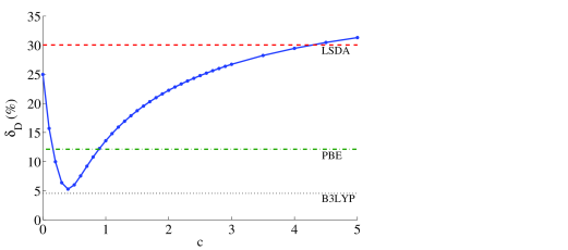
Figure 1: Average relative error of the dissociation energy, $\delta_{D}$, as a function of the parameter $c$ (solid line). Relative errors for the LSDA (dashed), PBE (dash-dotted) and B3LYP (dotted) functionals are given for comparison. Pure EXX reaches an error of $\delta^{EXX}_{D}(c)=66\%$ and exceeds the scale we chose here.

The functions $\delta_{D}(c)$ and $\delta_{E}(c)$ are plotted in Figs. 1 and 2, respectively, accompanied by the average relative errors for commonly used functionals: the LSDA, PBE, and B3LYP. As mentioned previously, the B3LYP results here and in the following were obtained in the generalized KS approach, which we, based on previous experience Kümmel and Kronik (2008), expect to yield total energies that are very similar to the ones from the KS approach for the systems studied here. For completeness, results obtained with pure EXX evaluated in the KLI approximation are also reported.

In both figures we observe clear minima for the proposed functional at the values of $c_{0}=0.4$ for $\delta_{D}$ and $0.6$ for $\delta_{E}$, with minimal error values of $5.3\%$ and $0.09\%$, respectively. These error values are close to those achieved with the B3LYP functional, and are significantly better than the PBE and LSDA results. Because optimizing $\delta_{D}(c)$ and $\delta_{E}(c)$ demands almost the same value for $c$, a satisfying description of both properties is possible using a common parameter of $c=0.5$. For this $c$, the relative error in the dissociation energy $\Delta D_{m}=(D_{m}-D^{exp})/D^{exp}$ is lowest for the BF molecule (0.7%) and highest for Li₂ and F₂ (14% and 17%, respectively). The relative error in the total energy is more evenly spread around 0.12%.

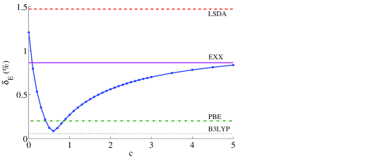
Figure 2: Average relative error of the total energy, $\delta_{E}$, as a function of the parameter $c$ (blue solid line). Relative errors for the LSDA (dashed), PBE (dash-dotted) and B3LYP (dotted) functionals, as well as pure EXX(KLI) (purple solid line) are given for comparison.

The function $\delta_{I}(c)$ shown in Fig. 3 exhibits a different behavior, reaching its minimum of 6 % at a higher value of $c\approx 4.5$. When evaluated at $c=0.5$, the average relative error is $\delta_{I}(c=0.5)=26\%$. Although lower than 31% for B3LYP and 42% for both LSDA and PBE, such a deviation is rather significant. Therefore, Fig. 3 suggests that in order to reach good agreement between the experimental IP and $-\varepsilon_{ho}$, a larger amount of EXX is required.

Interestingly, when calculating NH and BO, we observed that the highest occupied state changes with varying the parameter $c$ from $\varepsilon_{ho}=\varepsilon_{3\downarrow}$ to $\varepsilon_{5\uparrow}$ at approximately $c=0.7$ for NH, and from $\varepsilon_{6\downarrow}$ to $\varepsilon_{7\uparrow}$ at $c=1.6$ for the BO molecule. Such systems could therefore be good candidates for checking the functional’s ability to predict physically meaningful orbitals in the sense of Ref. Dauth et al. (2011).

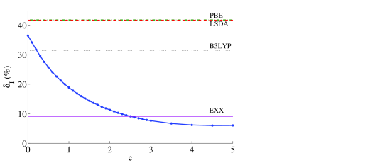
Figure 3: Average relative error of the IP predicted via the highest occupied KS eigenvalue, $\varepsilon_{ho}$, as a function of the parameter $c$ (blue solid line). Relative errors for the LSDA (dashed), PBE (dash-dotted) and B3LYP (dotted) functionals, as well as pure EXX(KLI) (purple solid line) are given for comparison.

Last, we checked the previously made assumption that experimental bond lengths can be used, assuming they are not very different from those obtained by relaxation. To this end, all 18 molecules in the reference set were relaxed, and the obtained bond lengths $L_{m}$ were compared to the experimental values, $L_{m}^{exp}$ Lide (2011). It was found that for most systems $L_{m}^{exp}$ lies within the computational error for $L_{m}$ and the difference $|L_{m}-L_{m}^{exp}|$ is below 0.02 Bohr , except F₂, where $|L_{m}-L_{m}^{exp}|\approx 0.08$ Bohr.

IV.4 Achievements of the suggested functional

In the following, we examine some of the proposed functional’s properties at the value of $c=0.5$, which was determined in Sec.IV.3.

As the functional is one-electron SI-free (see Sec. II), it is important to investigate its behavior in systems that are known to suffer from a large self-interaction error when described by standard DFAs. First, for one-electron systems, like H, He⁺, H${}_{2}^{+}$, etc. the functional reduces analytically to the EXX functional, as can be seen from Eq. (II). Therefore, all the properties of these systems are obtained, by construction, exactly. This advantage is not shared by (semi-)local or most hybrid functionals.

In particular, Fig. 4 presents the dissociation curve of H${}_{2}^{+}$, obtained with various functionals. It can be seen that, as expected, the curve obtained with the proposed functional perfectly agrees with the EXX curve, which provides the exact result in this case. In particular, our local hybrid does not exhibit a spurious maximum in the curve, which appears in conventional approximate functionals at bond lengths around 5-6 Bohr Bally and Sastry (1997); Ruzsinszky et al. (2005); Cohen et al. (2008); Livshits and Baer (2008); Nafziger and Wasserman (2013) and whose electrostatic origin has recently been discussed Dwyer and Tozer (2011). The dissociation of neutral H₂ is a special challenge for most density functionals and is closely connected to the question of how static correlation is accounted for Cohen et al. (2012). Our local hybrid for H₂ yields a binding curve that is qualitatively similar to the one obtained in pure exchange calculations, i.e., for large internuclear separation the lowest energy is obtained with a spin-polarized atomic density centered around each nucleus, which yields a total energy of 1 Hartree. Quantitatively, there are differences with respect to the EXX solution: The point from which on the spin-polarized solution has a lower energy than the spin-unpolarized one lies at about 3.6 Bohr with our local hybrid, and the minimum energy is -1.173 Hartree as compared to -1.134 Hartree obtained with EXX.

Figure 4: Dissociation curve of the H${}_{2}^{+}$ molecule, for the LSDA (squares), PBE (x’s), B3LYP (dots), EXX (solid line) and the suggested functional (circles).

Generally, delocalization in stretched molecular bonds is conceptually connected to the SI-error of DFAs Cohen et al. (2008). Therefore, reduction of this error marks a first step towards enhancing the description of dissociation processes and chemical reactions Ruzsinszky et al. (2006).

To examine this, the dissociation curve of the 3-electron molecule He${}_{2}^{+}$ is shown in Fig. 5. The curve achieved with the suggested functional is the closest to the reference result obtained with a highly accurate wavefunctions method (see Ref. Ruzsinszky et al. (2005) and references therein). Here again, only our local hybrid and the EXX curves do not possess the spurious maximum, which appears in the conventional approximations – LSDA, PBE and B3LYP around 4 Bohr. Unlike for the H${}_{2}^{+}$ system, here the proposed functional does not automatically reduce to the exact expression, and therefore the accurate prediction for He${}_{2}^{+}$ in Fig. 5 can be seen as a consequence of the strong reduction of SI-errors, in agreement with a previous study. Körzdörfer et al. (2008)

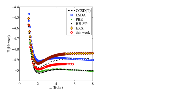
Figure 5: Dissociation curve of the He${}_{2}^{+}$ molecule, for the LSDA (squares), PBE (x’s), B3LYP (dots), EXX (rhombi), and the suggested functional with $c=0.5$ (circles), compared to CCSD(T) results from Ref. Ruzsinszky et al. (2005) (dashed line)

We further investigated how well $\varepsilon_{ho}$ corresponds to the experimental IP Lide (2011) for the atoms Li, Na, and K. These atoms can be considered as quasi-one-electron systems, consisting of electrons arranged in closed shells, which screen the charge of the nucleus, and one additional electron in the last open shell. Table 3 shows that the $\varepsilon_{ho}$ obtained from our functional evaluated with $c=0.5$ is closer to the experimental IP than the $\varepsilon_{ho}$ from LSDA, PBE, and B3LYP. Note that for these systems a remarkable improvement is achieved, as one would expect from their strong one-electron character.

Table 3: The highest occupied eigenvalue compared to the experimental IP for Li, Na, and K, computed with four different functionals (LSDA, PBE, B3LYP and our suggested functional using $c=0.5$). The table contains the absolute numbers in Hartree as well as the relative error in %.

	IP	$-\varepsilon_{ho}$
system	Exp.	LSDA	PBE	B3LYP	suggested functional
Li	$0.1981$	0.1163	0.1185	0.1311	0.1797
		(-41 %)	(-40 %)	(-34 %)	(-9 %)
Na	$0.1886$	0.1131	0.1116	0.1251	0.1647
		(-40 %)	(-41 %)	(-34 %)	(-13 %)
K	$0.1595$	0.0961	0.0930	0.1038	0.1334
		(-40 %)	(-42 %)	(-35 %)	(-16 %)

V Conclusions

In this article we presented the construction of a local hybrid functional that combines full exact exchange with compatible correlation. The functional respects the homogeneous electron gas limit and addresses the one-electron self-interaction error via a one-spin-orbital-region indicator. The qualitative improvement that is achieved with this construction is reflected in, e.g., dissociation energy curves for H${}_{2}^{+}$ and He${}_{2}^{+}$ that are much more realistic than the ones obtained from (semi-) local functionals and global hybrids. We investigated different conditions for fixing the undetermined parameter of the functional. When the parameter is fit to minimize binding energy errors or total energy errors, with respect to experiment, then our local hybrid reaches an accuracy that is better than LSDA or PBE and similar to the one afforded by the B3LYP global hybrid. Predicting the first ionization energy via the highest occupied eigenvalue $\varepsilon_{ho}$ is more accurate with our functional than with LSDA, PBE or B3LYP, but still not satisfactorily accurate.

When the parameter is fit such that $-\varepsilon_{ho}$ should be as close as possible to the experimental first ionization potential, then the local hybrid functional achieves much smaller errors in this quantity than, e.g., B3LYP. However, the value obtained for the free parameter differs considerably from the one that was obtained by fitting to binding or total energies. As a result, prediction of these energies considerably differs from their experimental values. Therefore, our local hybrid does allow for reaching accurate binding energies or accurate highest eigenvalues, but not with the same functional parametrization.

Looking at this from a more general perspective, we note that many functionals can achieve good accuracy on one of the aforementioned properties or the other, but not on both properties at the same time.

A first example are global hybrids. With the usual 0.2 to 0.25 fraction of exact exchange they yield good binding energies, but highest eigenvalues that are considerably too small in magnitude. Increasing the aforementioned fraction to $\sim 0.75$ leads to improved gap prediction Sai et al. (2011); Imamura et al. (2011); Atalla et al. (2013). However, such a large fraction of exact exchange can compromise significantly the accuracy in thermochemical Adamo and Barone (1999); Ernzerhof and Scuseria (1999); Zhao and Truhlar (2008) or electronic structure properties. Marom et al. (2010); Körzdörfer and Kümmel (2010); Kronik et al. (2012)

A second example are range-separated hybrid functionals. When combined with a tuning procedure based on the IP theorem Stein et al. (2010); Refaely-Abramson et al. (2011, 2012); Kronik et al. (2012); Körzdörfer et al. (2011); Sini et al. (2011); Foster and Wong (2012); Phillips et al. (2012); Risko and Brédas (2013), they allow for obtaining eigenvalues that reflect ionization potentials very accurately by construction. However, the typical value of the range-separation parameter that is reached by such tuning is quite different from the one that is reached when atomization energy errors are minimized via the range-separation parameter Livshits and Baer (2007).

A third example is provided by the various self-interaction correction schemes. Different forms of self-interaction correction greatly improve the interpretability of the eigenvalues when compared to semi-local functionals Perdew and Zunger (1981); Körzdörfer et al. (2009); Pederson et al. (1985); Klüpfel et al. (2012); Ullrich et al. (2000); Körzdörfer et al. (2008); Vydrov and Scuseria (2005), but binding energies are not accurately predicted Vydrov and Scuseria (2005); Hofmann et al. (2012) unless the correction is “scaled down” Vydrov et al. (2006); Klüpfel et al. (2012).

This rather universal difficulty to achieve accurate eigenvalues and accurate binding energies at the same time may indicate that combining these two properties may require a type of physics that all present day functionals lack Verma and Bartlett (2012).

Recent work provides two new and interesting perspectives on this problem. On the one hand, it has been noted that even a semi-local functional can yield eigenvalues that are qualitatively similar to the ones obtained from bare EXX when the asymptotic properties of a GGA are carefully determined Armiento and Kümmel (2013). On the other hand, it has recently been shown that an ensemble perspective offers new and improved ways of interpreting eigenvalues and extracting information from semi-local functionals Kraisler and Kronik (2013). Exploring in particular this latter option, i.e., combining the ensemble approach with the present local hybrid functional, will be the topic of future work and may shed further light on the question of how to obtain accurate binding energies and Kohn-Sham eigenvalues from the same functional.

Appendix A Derivation of the correlation potential

In order to employ the OEP formalism Grabo et al. (1997); Kümmel and Kronik (2008) (or its KLI approximation Krieger et al. (1992)), one has to provide an analytical expression for the functional derivative of the explicitly orbital-dependent exchange-correlation energy, $E_{xc}[\{\varphi_{i\sigma}\}]$, with respect to the orbitals $\{\varphi_{i\sigma}\}$. For the functional proposed in the present contribution,

$$E_{xc}[\{\varphi_{i\sigma}\}]=E_{x}^{ex}[\{\varphi_{i\sigma}\}]+E^{iso}_{c}[\{\varphi_{i\sigma}\}]+E_{c}^{sl}[\{\varphi_{i\sigma}\}],$$ (12)

where $E_{x}^{ex}[\{\varphi_{i\sigma}\}]$ is the exact exchange defined in Eq.(1), $E_{c}^{sl}[\{\varphi_{i\sigma}\}]$ is the semi-local correlation energy, whose energy density per particle, $e_{c}^{sl}(\mathbf{r})$, is given in Eq. (9), and $E^{iso}_{c}[\{\varphi_{i\sigma}\}]$ equals

$$E^{iso}_{c}[\{\varphi_{i\sigma}\}]=\int f(\mathbf{r}^{\prime})\,n(\mathbf{r}^{\prime})\,\left(e_{x}^{L\!S\!D\!A}(\mathbf{r}^{\prime})-e_{x}^{ex}(\mathbf{r}^{\prime})\right)\,\mathrm{d}^{3}r^{\prime},$$ (13)

with the LMF function, $f(\mathbf{r})$, being defined in Eq. (8).

Due to the additive structure of Eq. (12), the functional derivative

$$u_{i\sigma}(\mathbf{r})=\frac{1}{\varphi^{*}_{i\sigma}(\mathbf{r})}\frac{\delta E_{xc}[\{\varphi_{i\sigma}\}]}{\delta\varphi_{i\sigma}(\mathbf{r})}$$ (14)

can be split in three terms:

$$u_{i\sigma}(\mathbf{r})=u^{exx}_{i\sigma}(\mathbf{r})+u^{iso}_{i\sigma}(\mathbf{r})+u^{sl}_{i\sigma}(\mathbf{r}),$$ (15)

which are considered separately in the following.

A.1 The exact exchange contribution

The first term on the RHS of Eq. (15) can be computed directly from the exact-exchange expression (Eq. (1))

$$E_{x}^{ex}=-\frac{1}{2}\sum_{\begin{subarray}{c}i,j=1\\ \sigma=\uparrow,\downarrow\end{subarray}}^{N_{\sigma}}\int\int\frac{\varphi_{i\sigma}^{*}(\mathbf{r})\varphi_{j\sigma}(\mathbf{r})\varphi_{i\sigma}(\mathbf{r}^{\prime})\varphi_{j\sigma}^{*}(\mathbf{r}^{\prime})}{|\mathbf{r}-\mathbf{r}^{\prime}|}\,\mathrm{d}^{3}r\mathrm{d}^{3}r^{\prime}$$ (16)

and simply reads

$$\varphi^{*}_{i\sigma}(\mathbf{r})\,u^{exx}_{i\sigma}(\mathbf{r})=-\sum_{j=1}^{N_{\sigma}}\varphi_{j\sigma}^{*}(\mathbf{r})\int\frac{\varphi^{*}_{i\sigma}(\mathbf{r}^{\prime})\varphi_{j\sigma}(\mathbf{r}^{\prime})}{|\mathbf{r}-\mathbf{r}^{\prime}|}\,\mathrm{d}^{3}r^{\prime}.$$ (17)

A.2 The semi-local correlation contribution

The self-interaction-free semi-local correlation energy contribution $E_{c}^{sl}[\{\varphi_{i\sigma}\}]$ is defined by

$$E^{sl}_{c}[\{\varphi_{i\sigma}\}]=\int g(\mathbf{r}^{\prime})Q(\mathbf{r}^{\prime})\,\mathrm{d}^{3}r^{\prime},$$ (18)

where

$$g(\mathbf{r})=1-\frac{\tau_{W}(\mathbf{r})}{\tau(\mathbf{r})}\zeta^{2}(\mathbf{r})$$ (19)

and

$$Q(\mathbf{r})=n(\mathbf{r})e_{c}^{L\!S\!D\!A}(\mathbf{r}).$$ (20)

For completeness, we list out all the quantities that are required to construct the function $g(\mathbf{r})$:

1. kinetic energy density

   $$\tau(\mathbf{r})=\frac{1}{2}\sum_{\begin{subarray}{c}i=1\\ \sigma=\uparrow,\downarrow\end{subarray}}^{N_{\sigma}}|\nabla\varphi_{i\sigma}(\mathbf{r})|^{2};$$ (21)

2. Von Weizsäcker kinetic energy density

   $$\tau_{W}(\mathbf{r})=\frac{|\nabla n(\mathbf{r})|^{2}}{8n(\mathbf{r})}=\frac{1}{2}|\nabla n^{\frac{1}{2}}(\mathbf{r})|^{2};$$ (22)

3. spin polarization

   $$\zeta(\mathbf{r})=\frac{n_{\uparrow}(\mathbf{r})-n_{\downarrow}(\mathbf{r})}{n_{\uparrow}(\mathbf{r})+n_{\downarrow}(\mathbf{r})}$$

   .

Taking the functional derivative based on Eq. (18) results in two parts:

$$\varphi^{*}_{i\sigma}(\mathbf{r})u^{sl}_{i\sigma}(\mathbf{r}) = \int\left(\frac{\delta g(\mathbf{r}^{\prime})}{\delta\varphi_{i\sigma}(\mathbf{r})}\right)Q(\mathbf{r}^{\prime})\,\mathrm{d}^{3}r^{\prime}$$ (23)

$$+\int g(\mathbf{r}^{\prime})\left(\frac{\delta Q(\mathbf{r}^{\prime})}{\delta\varphi_{i\sigma}(\mathbf{r})}\right)\mathrm{d}^{3}r^{\prime}$$

By denoting the constituent functions of the function $g(\mathbf{r})$ by $\psi_{1}(\mathbf{r})=\tau(\mathbf{r})$, $\psi_{2}(\mathbf{r})=\tau_{W}(\mathbf{r})$ and $\psi_{3}(\mathbf{r})=\zeta(\mathbf{r})$, chain rule arguments lead to the following expression:

$$\left(\frac{\delta g(\mathbf{r}^{\prime})}{\delta\varphi_{i\sigma}(\mathbf{r})}\right)=\sum_{l=1}^{3}\frac{\delta\psi_{l}(\mathbf{r}^{\prime})}{\delta\varphi_{i\sigma}(\mathbf{r})}\frac{\delta g(\mathbf{r}^{\prime})}{\delta\psi_{l}(\mathbf{r}^{\prime})}$$ (24)

Here we explicitly took into account the fact that $g(\mathbf{r})$ depends on $\psi_{l}(\mathbf{r})$ locally.

In order to obtain an analytical expression for $\delta g(\mathbf{r}^{\prime})/\delta\varphi_{i\sigma}(\mathbf{r})$, which can then be inserted into Eq. (23), one has to consider the three constituent functions $\psi_{l}(\mathbf{r})$ separately:

$l=1:$

$$\frac{\delta\tau(\mathbf{r}^{\prime})}{\delta\varphi_{i\sigma}(\mathbf{r})} =-\frac{1}{2}\delta(\mathbf{r}-\mathbf{r}^{\prime})\left[\nabla^{\prime 2}\varphi^{*}_{i\sigma}(\mathbf{r}^{\prime})+(\nabla^{\prime}\varphi^{*}_{i\sigma}(\mathbf{r}^{\prime}))\cdot\nabla^{\prime}\right]$$ (25)

$$\frac{\delta g(\mathbf{r}^{\prime})}{\delta\tau(\mathbf{r}^{\prime})} =\frac{\tau_{W}(\mathbf{r}^{\prime})\zeta^{2}(\mathbf{r}^{\prime})}{\tau^{2}(\mathbf{r}^{\prime})}$$ (26)

$l=2:$

$$\frac{\delta\tau_{W}(\mathbf{r}^{\prime})}{\delta\varphi_{i\sigma}(\mathbf{r})} =-\frac{\varphi^{*}_{i\sigma}(\mathbf{r}^{\prime})}{2n^{\frac{1}{2}}(\mathbf{r}^{\prime})} \!\!\!\delta(\mathbf{r}-\mathbf{r}^{\prime})\left(\nabla^{\prime 2}(n^{\frac{1}{2}}(\mathbf{r}^{\prime}))+\right.$$

$$\left.(\nabla^{\prime}n^{\frac{1}{2}}(\mathbf{r}^{\prime}))\cdot\nabla^{\prime}\right)$$ (27)

$$\frac{\delta g(\mathbf{r}^{\prime})}{\delta\tau_{W}(\mathbf{r}^{\prime})} =-\frac{\zeta^{2}(\mathbf{r}^{\prime})}{\tau(\mathbf{r}^{\prime})}$$ (28)

$l=3:$

$$\frac{\delta\zeta(\mathbf{r}^{\prime})}{\delta\varphi_{i\sigma}(\mathbf{r})} = \varphi^{*}_{i\sigma}(\mathbf{r}^{\prime})\delta(\mathbf{r}-\mathbf{r}^{\prime})\left(\frac{\delta_{\sigma}-\zeta(\mathbf{r}^{\prime})}{n(\mathbf{r}^{\prime})}\right)$$ (29)

$$\frac{\delta g(\mathbf{r}^{\prime})}{\delta\zeta(\mathbf{r}^{\prime})} = -\frac{2\tau_{W}(\mathbf{r}^{\prime})\zeta(\mathbf{r}^{\prime})}{\tau(\mathbf{r}^{\prime})}$$ (30)

Here the operator $\nabla^{\prime}$ denotes a gradient relative to the coordinate $(\mathbf{r}^{\prime})$ and the quantity $\delta_{\sigma}$ distinguishes between the two spin channels by

$$\delta_{\sigma}=\begin{cases}\,\,\,\,1&\text{if }\sigma=\uparrow\\ -1&\text{if }\sigma=\downarrow.\end{cases}$$ (31)

It is noted that the functional derivatives above have the presented form with respect to the occupied orbitals only; derivatives with respect to unoccupied orbitals equal zero.

The derived relations (25) - (30) now have to be inserted via Eq. (24) into Eq. (23). By further employing a chain rule argument for the second term on the RHS of Eq. (23)

$$\frac{\delta Q(\mathbf{r}^{\prime})}{\delta\varphi_{i\sigma}(\mathbf{r})} = \sum_{\tau=\uparrow,\downarrow}\int\frac{\delta Q(\mathbf{r}^{\prime})}{\delta n_{\tau}(\mathbf{r}^{\prime\prime})}\frac{\delta n_{\tau}(\mathbf{r}^{\prime\prime})}{\delta\varphi_{i\sigma}(\mathbf{r})}\,\mathrm{d}^{3}r^{\prime\prime}$$

$$= \varphi^{*}_{i\sigma}(\mathbf{r})\frac{\delta Q(\mathbf{r}^{\prime})}{\delta n_{\sigma}(\mathbf{r})}=\varphi^{*}_{i\sigma}(\mathbf{r})v_{c,\sigma}^{L\!S\!D\!A}(\mathbf{r}^{\prime})\delta(\mathbf{r}-\mathbf{r}^{\prime}),$$

one arrives at the final expression of the functional derivative of $E_{c}^{sl}[\{\varphi_{i\sigma}\}]$:

$$\varphi^{*}_{i\sigma}(\mathbf{r})u^{sl}_{i\sigma}(\mathbf{r})=$$

$$-\frac{1}{2}\left[\left(\nabla^{2}\varphi^{*}_{i\sigma}(\mathbf{r})\right)\frac{\delta g(\mathbf{r})}{\delta\tau(\mathbf{r})}Q(\mathbf{r})+\nabla\varphi^{*}_{i\sigma}(\mathbf{r})\cdot\nabla\left(\frac{\delta g(\mathbf{r})}{\delta\tau(\mathbf{r})}Q(\mathbf{r})\right)\right]$$

$$-\frac{\varphi^{*}_{i\sigma}(\mathbf{r})}{2n^{\frac{1}{2}}(\mathbf{r})}\left[\left(\nabla^{2}n^{\frac{1}{2}}(\mathbf{r})\right)\frac{\delta g(\mathbf{r})}{\delta\tau_{W}(\mathbf{r})}Q(\mathbf{r})+\right.$$

$$\hskip 128.0374pt\left.\nabla n^{\frac{1}{2}}(\mathbf{r})\cdot\nabla\left(\frac{\delta g(\mathbf{r})}{\delta\tau_{W}(\mathbf{r})}Q(\mathbf{r})\right)\right]$$

$$+\varphi^{*}_{i\sigma}(\mathbf{r})\ \left(\delta_{\sigma}-\zeta(\mathbf{r})\right)\frac{\delta g(\mathbf{r})}{\delta\zeta(\mathbf{r})}e^{L\!S\!D\!A}_{c}(\mathbf{r})$$

$$+\varphi^{*}_{i\sigma}(\mathbf{r})\,g(\mathbf{r})\ v_{c,\sigma}^{L\!S\!D\!A}(\mathbf{r})$$ (33)

Equation (33) corresponds to the functional derivative the way it was implemented into the KLI/OEP-routine in the program package DARSEC.

A.3 The contribution $E^{iso}_{c}[\{\varphi_{i\sigma}\}]$

The correlation term $E^{iso}_{c}[\{\varphi_{i\sigma}\}]$ is defined in Eq. (13). Let us denote

$$P(\mathbf{r})=n(\mathbf{r})\left(e_{x}^{L\!S\!D\!A}(\mathbf{r})-e_{x}^{ex}(\mathbf{r})\right)$$ (34)

and recall that the LMF function $f(\mathbf{r})$ equals

$$f(\mathbf{r})=\frac{1-\frac{\tau_{W}(\mathbf{r})}{\tau(\mathbf{r})}\zeta^{2}(\mathbf{r})}{1+c\cdot t^{2}(\mathbf{r})}$$ (35)

In addition to the quantities $\tau$, $\tau_{W}$ and $\zeta$ introduced above, the function $f(\mathbf{r})$ additionally employs the so-called reduced density gradient Perdew et al. (1996a)

$$t(\mathbf{r}) = \left(\frac{\pi}{3}\right)^{\frac{1}{6}}\frac{a_{0}^{\frac{1}{2}}}{4\Phi(\mathbf{r})}\frac{|\nabla n(\mathbf{r})|}{n^{\frac{7}{6}}(\mathbf{r})}$$ (36)

$$:= a\frac{t_{n}(\mathbf{r})}{\Phi(\mathbf{r})}$$

with

$$\Phi(\mathbf{r})=\frac{1}{2}\left[\left(1+\zeta(\mathbf{r})\right)^{\frac{2}{3}}+\left(1-\zeta(\mathbf{r})\right)^{\frac{2}{3}}\right]$$ (37)

and

$$a=\left(\frac{\pi}{3}\right)^{\frac{1}{6}}\frac{a_{0}^{\frac{1}{2}}}{4}=const.$$

The exact relation

$$t_{n}^{2}(\mathbf{r})=\frac{8\tau_{W}(\mathbf{r})}{n^{\frac{4}{3}}(\mathbf{r})}$$ (38)

will be useful for later derivations.

Analogously to Eq. (23), the application of the functional derivative with respect to the KS-orbitals leads to two contributions:

$$\varphi^{*}_{i\sigma}(\mathbf{r})u^{iso}_{i\sigma}(\mathbf{r}) = \int\left(\frac{\delta f(\mathbf{r}^{\prime})}{\delta\varphi_{i\sigma}(\mathbf{r})}\right)P(\mathbf{r}^{\prime})\,\mathrm{d}^{3}r^{\prime}$$ (39)

$$+\int f(\mathbf{r}^{\prime})\left(\frac{\delta P(\mathbf{r}^{\prime})}{\delta\varphi_{i\sigma}(\mathbf{r})}\right)\mathrm{d}^{3}r^{\prime}$$

Moreover, an analogous relation to Eq. (24) helps to rewrite the first part of this equation, only that now one has to consider also the functions $\psi_{4}(\mathbf{r})=t_{n}^{2}(\mathbf{r})$ and $\psi_{5}(\mathbf{r})=\Phi(\mathbf{r})$:

$$\left(\frac{\delta f(\mathbf{r}^{\prime})}{\delta\varphi_{i\sigma}(\mathbf{r})}\right)=\sum_{l=1}^{5}\frac{\delta\psi_{l}(\mathbf{r}^{\prime})}{\delta\varphi_{i\sigma}(\mathbf{r})}\frac{\delta f(\mathbf{r}^{\prime})}{\delta\psi_{l}(\mathbf{r}^{\prime})}$$ (40)

We evaluate each term separately and obtain:
$l=1:$

$$\frac{\delta f(\mathbf{r}^{\prime})}{\delta\tau(\mathbf{r}^{\prime})}=\frac{\frac{\tau_{W}(\mathbf{r}^{\prime})}{\tau^{2}(\mathbf{r}^{\prime})}\zeta^{2}(\mathbf{r}^{\prime})}{1+c\cdot t^{2}(\mathbf{r}^{\prime})}=-\frac{\delta f(\mathbf{r}^{\prime})}{\delta\tau_{W}(\mathbf{r}^{\prime})}\frac{\tau_{W}(\mathbf{r}^{\prime})}{\tau(\mathbf{r}^{\prime})}$$ (41)

$l=2:$

$$\frac{\delta f(\mathbf{r}^{\prime})}{\delta\tau_{W}(\mathbf{r}^{\prime})}=-\frac{\zeta^{2}(\mathbf{r}^{\prime})}{\tau(\mathbf{r}^{\prime})\left(1+c\cdot t^{2}(\mathbf{r}^{\prime})\right)}$$ (42)

$l=3:$

$$\frac{\delta f(\mathbf{r}^{\prime})}{\delta\zeta(\mathbf{r}^{\prime})}=-\frac{2\frac{\tau_{W}(\mathbf{r}^{\prime})}{\tau(\mathbf{r}^{\prime})}\zeta(\mathbf{r}^{\prime})}{1+c\cdot t^{2}(\mathbf{r}^{\prime})}$$ (43)

$l=4:$

$$\frac{\delta t_{n}^{2}(\mathbf{r}^{\prime})}{\delta\varphi_{i\sigma}(\mathbf{r})}=8\frac{\delta\tau_{W}(\mathbf{r}^{\prime})}{\delta\varphi_{i\sigma}(\mathbf{r})}\frac{1}{n^{\frac{4}{3}}(\mathbf{r}^{\prime})}-\frac{32}{3}\frac{\tau_{W}(\mathbf{r}^{\prime})\varphi^{*}_{i\sigma}(\mathbf{r}^{\prime})}{n^{\frac{7}{3}}(\mathbf{r}^{\prime})}\delta(\mathbf{r}-\mathbf{r}^{\prime})$$ (44)

$$\frac{\delta f(\mathbf{r}^{\prime})}{\delta t_{n}^{2}(\mathbf{r}^{\prime})}=-\frac{ca^{2}f(\mathbf{r}^{\prime})}{\Phi^{2}(\mathbf{r}^{\prime})\left(1+c\cdot t^{2}(\mathbf{r}^{\prime})\right)}$$ (45)

$l=5:$

$$\frac{\delta\Phi(\mathbf{r}^{\prime})}{\delta\varphi_{i\sigma}(\mathbf{r})} = \frac{\delta\Phi(\mathbf{r}^{\prime})}{\delta\zeta(\mathbf{r}^{\prime})}\frac{\delta\zeta(\mathbf{r}^{\prime})}{\delta\varphi_{i\sigma}(\mathbf{r})}$$ (46)

$$= \frac{1}{3}\left[\left(1+\zeta(\mathbf{r}^{\prime})\right)^{-\frac{1}{3}}-\left(1-\zeta(\mathbf{r}^{\prime})\right)^{-\frac{1}{3}}\right]\cdot$$

$$\varphi^{*}_{i\sigma}(\mathbf{r}^{\prime})\delta(\mathbf{r}-\mathbf{r}^{\prime})\left(\frac{\delta_{\sigma}-\zeta(\mathbf{r}^{\prime})}{n(\mathbf{r}^{\prime})}\right)$$

To avoid numerical instability due to the negative powers of $-\frac{1}{3}$, we multiply the above relation by $(1+\zeta(\mathbf{r}^{\prime}))^{\frac{1}{3}}(1-\zeta(\mathbf{r}^{\prime}))^{\frac{1}{3}}$ and then divide by the same term expressed in terms of the spin-densities. We then obtain

$$\frac{\delta\Phi(\mathbf{r}^{\prime})}{\delta\varphi_{i\sigma}(\mathbf{r})}=-\frac{1}{3}\left[\left(1+\zeta(\mathbf{r}^{\prime})\right)^{\frac{1}{3}}-\left(1-\zeta(\mathbf{r}^{\prime})\right)^{\frac{1}{3}}\right]\cdot$$

$$\hskip 34.14322pt\frac{n^{\frac{2}{3}}(\mathbf{r}^{\prime})}{2^{\frac{2}{3}}\left(n_{\uparrow}(\mathbf{r}^{\prime})n_{\downarrow}(\mathbf{r}^{\prime})\right)^{\frac{1}{3}}}\varphi^{*}_{i\sigma}(\mathbf{r}^{\prime})\cdot\delta(\mathbf{r}-\mathbf{r}^{\prime})\left(\frac{\delta_{\sigma}-\zeta(\mathbf{r}^{\prime})}{n(\mathbf{r}^{\prime})}\right)$$ (47)

$$\frac{\delta f(\mathbf{r}^{\prime})}{\delta\Phi(\mathbf{r}^{\prime})}=\frac{2ct^{2}(\mathbf{r}^{\prime})f(\mathbf{r}^{\prime})}{\Phi(\mathbf{r}^{\prime})\left(1+c\cdot t^{2}(\mathbf{r}^{\prime})\right)}$$ (48)

In order to compute the first term of Eq. (39), one now has to evaluate all the contributions originating from the different $\psi_{l}$ (Eqs. (25), (27), (29), (41), (42), (43), (44), (45), (47), (48)) via the chain rule argument (40).

Similar considerations are now used for the second term on the RHS Eq. (39). By applying chain rule arguments only to the semi-local energy density part of $P(\mathbf{r})$, one arrives at the following equation:

$$\frac{\delta P(\mathbf{r}^{\prime})}{\delta\varphi_{i\sigma}(\mathbf{r})} = \sum_{\tau=\uparrow,\downarrow}\int\frac{\delta\left(n(\mathbf{r}^{\prime})e_{x}^{L\!S\!D\!A}(\mathbf{r}^{\prime})\right)}{\delta n_{\tau}(\mathbf{r}^{\prime\prime})}\frac{\delta n_{\tau}(\mathbf{r}^{\prime\prime})}{\delta\varphi_{i\sigma}(\mathbf{r})}\,\mathrm{d}^{3}r^{\prime\prime}$$ (49)

$$-\frac{\delta\left(n(\mathbf{r}^{\prime})e_{x}^{ex}(\mathbf{r}^{\prime})\right)}{\delta\varphi_{i\sigma}(\mathbf{r})}$$

While the first term contributes simply via the regular density-dependent LSDA exchange potential (similar to Eq. (LABEL:secondpart)), requires the second term explicit evaluation of the exact exchange energy density

$$n(\mathbf{r}^{\prime})e_{x}^{ex}(\mathbf{r}^{\prime})\!\!=\!\!-\frac{1}{2}\!\!\sum_{\begin{subarray}{c}k,q=1\\ \upsilon=\uparrow,\downarrow\end{subarray}}^{N_{\upsilon}}\!\!\int\!\!\frac{\varphi_{k\upsilon}^{*}(\mathbf{r}^{\prime})\varphi_{q\upsilon}(\mathbf{r}^{\prime})\varphi_{k\upsilon}(\mathbf{r}^{\prime\prime})\varphi_{q\upsilon}^{*}(\mathbf{r}^{\prime\prime})}{|\mathbf{r}^{\prime}-\mathbf{r}^{\prime\prime}|}\mathrm{d}^{3}r^{\prime\prime}.$$ (50)

Therefore, Eq. (49) results in

$$\frac{\delta P(\mathbf{r}^{\prime})}{\delta\varphi_{i\sigma}(\mathbf{r})} = \varphi^{*}_{i\sigma}(\mathbf{r})v_{x,\sigma}^{L\!S\!D\!A}(\mathbf{r}^{\prime})\delta(\mathbf{r}-\mathbf{r}^{\prime})$$ (51)

$$+ \frac{1}{2}\sum_{k=1}^{N_{\sigma}}\delta(\mathbf{r}-\mathbf{r}^{\prime})\varphi_{k\sigma}^{*}(\mathbf{r}^{\prime})\int\frac{\varphi_{k\sigma}(\mathbf{r}^{\prime\prime})\varphi_{i\sigma}^{*}(\mathbf{r}^{\prime\prime})}{|\mathbf{r}^{\prime}-\mathbf{r}^{\prime\prime}|}\,\mathrm{d}^{3}r^{\prime\prime}$$

$$+ \frac{1}{2}\sum_{q=1}^{N_{\sigma}}\frac{\varphi_{i\sigma}^{*}(\mathbf{r}^{\prime})\varphi_{q\sigma}(\mathbf{r}^{\prime})\varphi_{q\sigma}^{*}(\mathbf{r})}{|\mathbf{r}^{\prime}-\mathbf{r}|}.$$

Evaluating this expression with the corresponding integral in Eq. (39) and adding the previously derived first term, one arrives at the final expression for the functional derivative of $E^{iso}_{c}[\{\varphi\}]$ with respect to the KS orbitals:

$$\varphi^{*}_{i\sigma}(\mathbf{r})u^{iso}_{i\sigma}(\mathbf{r})=-\frac{f(\mathbf{r})}{2}\varphi^{*}_{i\sigma}(\mathbf{r})\,u^{exx}_{i\sigma}(\mathbf{r})+\frac{1}{2}\sum_{j=1}^{N_{\sigma}}\varphi^{*}_{j\sigma}(\mathbf{r})\int f(\mathbf{r}^{\prime})\frac{\varphi_{i\sigma}^{*}(\mathbf{r}^{\prime})\varphi_{j\sigma}(\mathbf{r}^{\prime})}{|\mathbf{r}-\mathbf{r}^{\prime}|}\,\mathrm{d}^{3}r^{\prime}+\varphi^{*}_{i\sigma}(\mathbf{r})f(\mathbf{r})v_{x,\sigma}^{L\!S\!D\!A}(\mathbf{r})$$

$$-\frac{1}{2}\left[\left(\nabla^{2}\varphi^{*}_{i\sigma}(\mathbf{r})\right)\frac{\delta f(\mathbf{r})}{\delta\tau(\mathbf{r})}P(\mathbf{r})+\nabla\varphi^{*}_{i\sigma}(\mathbf{r})\cdot\nabla\left(\frac{\delta f(\mathbf{r})}{\delta\tau(\mathbf{r})}P(\mathbf{r})\right)\right]-\frac{\varphi^{*}_{i\sigma}(\mathbf{r})}{2n^{\frac{1}{2}}(\mathbf{r})}\left[\left(\nabla^{2}n^{\frac{1}{2}}(\mathbf{r})\right)\frac{\delta f(\mathbf{r})}{\delta\tau_{W}(\mathbf{r})}P(\mathbf{r})+\right.$$

$$\hskip 341.43306pt\left.\nabla n^{\frac{1}{2}}(\mathbf{r})\cdot\nabla\left(\frac{\delta f(\mathbf{r})}{\delta\tau_{W}(\mathbf{r})}P(\mathbf{r})\right)\right]$$

$$-\frac{1}{3}\left[\left(1+\zeta(\mathbf{r})\right)^{\frac{1}{3}}-\left(1-\zeta(\mathbf{r})\right)^{\frac{1}{3}}\right]\frac{\varphi^{*}_{i\sigma}(\mathbf{r})n^{\frac{2}{3}}(\mathbf{r})}{2^{\frac{2}{3}}\left(n_{\uparrow}(\mathbf{r})n_{\downarrow}(\mathbf{r})\right)^{\frac{1}{3}}}\left({\delta_{\sigma}-\zeta(\mathbf{r})}\right)\frac{\delta f(\mathbf{r})}{\delta\Phi(\mathbf{r})}\left(e^{L\!S\!D\!A}_{x}(\mathbf{r})-e^{ex}_{x}(\mathbf{r})\right)$$

$$-\frac{2\varphi^{*}_{i\sigma}(\mathbf{r})}{n^{\frac{4}{3}}(\mathbf{r})}\left[\nabla^{2}n(\mathbf{r})\left(e^{L\!S\!D\!A}_{x}(\mathbf{r})-e^{ex}_{x}(\mathbf{r})\right)\frac{\delta f(\mathbf{r})}{\delta t_{n}^{2}(\mathbf{r})}-\frac{28}{3}\tau_{W}(\mathbf{r})\left(e^{L\!S\!D\!A}_{x}(\mathbf{r})-e^{ex}_{x}(\mathbf{r})\right)\frac{\delta f(\mathbf{r})}{\delta t_{n}^{2}(\mathbf{r})}+\right.$$

$$\hskip 284.52756pt\left.\nabla n(\mathbf{r})\cdot\nabla\left(\left(e^{L\!S\!D\!A}_{x}(\mathbf{r})-e^{ex}_{x}(\mathbf{r})\right)\frac{\delta f(\mathbf{r})}{\delta t_{n}^{2}(\mathbf{r})}\right)\right]$$

$$+\varphi^{*}_{i\sigma}(\mathbf{r})\cdot\frac{2ct^{2}(\mathbf{r})}{1+ct^{2}(\mathbf{r})}f(\mathbf{r})\left(e^{L\!S\!D\!A}_{x}(\mathbf{r})-e^{ex}_{x}(\mathbf{r})\right)+\varphi^{*}_{i\sigma}(\mathbf{r})\left({\delta_{\sigma}-\zeta(\mathbf{r})}\right)\frac{\delta f(\mathbf{r})}{\delta\zeta(\mathbf{r})}\left(e^{L\!S\!D\!A}_{x}(\mathbf{r})-e^{ex}_{x}(\mathbf{r})\right)$$ (52)

Finally, we note that when numerically implementing such complex expressions, questions of numerical stability may emerge. We found that implementing the von Weizsäcker kinetic energy density as $\tau_{W}(\mathbf{r})=\frac{1}{2}|\nabla n^{\frac{1}{2}}(\mathbf{r})|^{2}$ and the quantity $\frac{\delta\Phi(\mathbf{r}^{\prime})}{\delta\varphi_{i\sigma}(\mathbf{r})}$ as in Eq. (47) is highly advantageous. In addition, we store $\tau_{W}(\mathbf{r})/\tau(\mathbf{r})$ as a separate quantity, enforcing the exact condition that it is never larger than 1. We also store separately the quantity $(1+ct^{2}(\mathbf{r}))^{-1}$ and express $ct^{2}(\mathbf{r})/(1+ct^{2}(\mathbf{r}))$ in terms of the former, to avoid the divergence of $t(\mathbf{r})$ at large distances.

Appendix B OEP/KLI comparison

This Appendix reports detailed numerical results for the total energies, $E_{tot}$, as well as the eigenvalues of the highest occupied KS state, $\varepsilon_{ho}$, using the proposed local hybrid functional for selected systems: the BH, Li₂, NH, and the N₂ molecules, as well as the C atom. A multiplicative, local KS potential was obtained by employing the functional derivative of Eq. (52) either in the full OEP scheme or by the KLI approximation. Table 4 lists the absolute values of $E_{tot}$ for KLI and OEP, as well as the differences between results obtained with both schemes. Table 5 provides the same comparsion for $\varepsilon_{ho}$.

Note that the systems BH, Li₂, and N₂ are spin-unpolarized. Therefore, for $c=0$ the functional reduces to the LSDA xc functional (cf. Eq. (II)) and thus no difference between KLI and OEP should occur. This is indeed the case, within numerical accuracy.

Table 4: Comparison of total energy, $E_{tot}$, using the suggested local hybrid functional in both the KLI and OEP schemes, as a function of $c$. All values are in Hartree.

system	$c$	KLI	OEP	$E^{KLI}_{tot}-E^{OEP}_{tot}$
C	0	-37.4804	-37.4804	0.0000
	0.5	-37.8108	-37.8110	0.0002
	2.5	-37.9494	-37.9497	0.0003
BH	0	-24.9768	-24.9768	0.0000
	0.5	-25.2612	-25.2614	0.0002
	2.5	-25.3983	-25.3988	0.0005
Li2	0	-14.7244	-14.7244	0.0000
	0.5	-14.9809	-14.9810	0.0001
	2.5	-15.1245	-15.1247	0.0002
NH	0	-54.7769	-54.7770	0.0001
	0.5	-55.1769	-55.1774	0.0005
	2.5	-55.3555	-55.3563	0.0008
N2	0	-108.6958	-108.6958	0.0000
	0.5	-109.4464	-109.4474	0.0009
	2.5	-109.7593	-109.7609	0.0017

Table 5: Comparison of highest occupied orbital energy $\varepsilon_{ho}$ using the suggested local hybrid functional in both the KLI and OEP schemes, as a function of $c$. All values are in Hartree.

system	$c$	KLI	OEP	$\varepsilon^{KLI}_{ho}-\varepsilon^{OEP}_{ho}$
C	0	-0.2740	-0.2736	-0.0005
	0.5	-0.3067	-0.3068	0.0001
	2.5	-0.3688	-0.3691	0.0003
BH	0	-0.2031	-0.2031	0.0000
	0.5	-0.2412	-0.2415	0.0003
	2.5	-0.3043	-0.3047	0.0004
Li2	0	-0.1189	-0.1189	0.0000
	0.5	-0.1286	-0.1289	0.0002
	2.5	-0.1522	-0.1527	0.0005
NH	0	-0.3157	-0.3164	0.0007
	0.5	-0.3770	-0.3783	0.0013
	2.5	-0.4581	-0.4607	0.0025
N2	0	-0.3825	-0.3825	0.0000
	0.5	-0.4456	-0.4447	-0.0010
	2.5	-0.5463	-0.5444	-0.0019

References

- Hohenberg and Kohn (1964) P. Hohenberg and W. Kohn, Phys. Rev. 136, B864 (1964).
- Kohn and Sham (1965) W. Kohn and L. J. Sham, Phys. Rev. 140, A1133 (1965).
- Parr and Yang (1989) R. G. Parr and W. Yang, Density-Functional Theory of Atoms and Molecules (Oxford University Press, New York, 1989).
- Dreizler and Gross (1995) R. Dreizler and E. K. U. Gross, eds., Density Functional Theory (Plenum Press, New York and London, 1995).
- Fiolhais et al. (2003) C. Fiolhais, F. Nogueira, and M. A. Marques, eds., A Primer in Density Functional Theory (Springer, 2003), vol. 620 of Lectures in Physics.
- Kurth and Perdew (2000) S. Kurth and J. P. Perdew, Int. J. Quantum Chem. 77, 814 (2000).
- Burke (2012) K. Burke, J. Chem. Phys. 136, 150901 (2012).
- Perdew and Schmidt (2001) J. P. Perdew and K. Schmidt, in Density Functional Theory and Its Application to Materials, edited by V. Van Doren, C. Van Alsenoy, and P. Geerlings (AIP, Melville NY, 2001).
- Ceperley and Alder (1980) D. Ceperley and B. Alder, Phys. Rev. Lett. 45, 566 (1980).
- Perdew and Wang (1992) J. P. Perdew and Y. Wang, Phys. Rev. B 45, 13244 (1992).
- Perdew and Zunger (1981) J. P. Perdew and A. Zunger, Phys. Rev. B 23, 5048 (1981).
- Vosko et al. (1980) S. H. Vosko, L. Wilk, and M. Nusair, Can. J. Phys. 58, 1200 (1980).
- Perdew and Wang (1986) J. P. Perdew and Y. Wang, Phys. Rev. B 33, 8800 (1986).
- Becke (1988) A. D. Becke, Phys. Rev. A 38, 3098 (1988).
- Lee et al. (1988) C. Lee, W. Yang, and R. G. Parr, Phys. Rev. B 37, 785 (1988).
- Perdew (1991) J. Perdew, in Electronic Structure of Solids ’91 , eds. P. Ziesche and H. Eschrig (Akademie Verlag, Berlin, 1991).
- Perdew et al. (1996a) J. P. Perdew, K. Burke, and M. Ernzerhof, Phys. Rev. Lett. 77, 3865 (1996a).
- Wu and Cohen (2006) Z. Wu and R. Cohen, Phys. Rev. B 73, 235116 (2006).
- Haas et al. (2011) P. Haas, F. Tran, P. Blaha, and K. Schwarz, Phys. Rev. B 83, 205117 (2011).
- Becke (1993a) A. D. Becke, J. Chem. Phys. 98, 1372 (1993a).
- Becke (1993b) A. D. Becke, J. Chem. Phys. 98, 5648 (1993b).
- Perdew et al. (1996b) J. P. Perdew, M. Ernzerhof, and K. Burke, J. Chem. Phys. 105, 9982 (1996b).
- Stephens et al. (1994) P. J. Stephens, F. J. Devlin, C. F. Chabalowski, and M. J. Frisch, J. Phys. Chem. 98, 11623 (1994).
- Adamo and Barone (1999) C. Adamo and V. Barone, J. Chem. Phys. 110, 6158 (1999).
- Ernzerhof and Scuseria (1999) M. Ernzerhof and G. E. Scuseria, J. Chem. Phys. 110, 5029 (1999).
- Grabo et al. (1997) T. Grabo, T. Kreibich, and E. K. U. Gross, Mol. Eng. 7, 27 (1997).
- Engel and Dreizler (2011) E. Engel and R. Dreizler, Density Functional Theory: An Advanced Course (Springer, 2011).
- Kümmel and Kronik (2008) S. Kümmel and L. Kronik, Rev. Mod. Phys. 80, 3 (2008).
- Perdew and Levy (1983) J. P. Perdew and M. Levy, Phys. Rev. Lett. 51, 1884 (1983).
- Tozer and Handy (1998) D. Tozer and N. C. Handy, J. Chem. Phys. 109, 10180 (1998).
- Perdew et al. (1982) J. P. Perdew, R. G. Parr, M. Levy, and J. L. Balduz, Phys. Rev. Lett. 49, 1691 (1982).
- Levy et al. (1984) M. Levy, J. P. Perdew, and V. Sahni, Physical Review A 30, 2745 (1984).
- Almbladh and von Barth (1985) C.-O. Almbladh and U. von Barth, Phys. Rev. B 31, 3231 (1985).
- Perdew and Levy (1997) J. P. Perdew and M. Levy, Phys. Rev. B 56, 16021 (1997).
- Stowasser and Hoffmann (1999) R. Stowasser and R. Hoffmann, J. Am. Chem. Soc. 121, 3414 (1999).
- Chong et al. (2002) D. P. Chong, O. V. Gritsenko, and E. J. Baerends, J. Chem. Phys. 116, 1760 (2002).
- Körzdörfer et al. (2009) T. Körzdörfer, S. Kümmel, N. Marom, and L. Kronik, Phys. Rev. B 79, 201205(R) (2009).
- Körzdörfer et al. (2010) T. Körzdörfer, S. Kümmel, N. Marom, and L. Kronik, Phys. Rev. B 82, 129903(E) (2010).
- Dauth et al. (2011) M. Dauth, T. Körzdörfer, S. Kümmel, J. Ziroff, M. Wiessner, A. Schöll, F. Reiner, M. Arita, and K. Shimada, Phys. Rev. Lett. 107, 193002 (2011).
- Bleiziffer et al. (2013) P. Bleiziffer, A. Heßelmann, and A. Görling, J. Chem. Phys. 139, 084113 (2013).
- Cohen and Chelikowsky (1988) M. Cohen and J. Chelikowsky, Electronic Structure and Optical Properties of Semiconductors (Springer-Verlag, Berlin, 1988).
- Dori et al. (2006) N. Dori, M. Menon, L. Kilian, M. Sokolowski, L. Kronik, and E. Umbach, Phys. Rev. B 73, 195208 (2006).
- Mundt et al. (2006) M. Mundt, S. Kümmel, B. Huber, and M. Moseler, Phys. Rev. B 73, 205407 (2006).
- Mundt and Kümmel (2007) M. Mundt and S. Kümmel, Phys. Rev. B 76, 035413 (2007).
- Körzdörfer and Kümmel (2010) T. Körzdörfer and S. Kümmel, Phys. Rev. B 82, 155206 (2010).
- Marom et al. (2008) N. Marom, O. Hod, G. E. Scuseria, and L. Kronik, J. Chem. Phys. 128, 164107 (2008).
- Marom and Kronik (2009) N. Marom and L. Kronik, Appl. Phys. A 95, 159 (2009).
- Marom et al. (2010) N. Marom, A. Tktchenko, M. Scheffler, and L. Kronik, J. Chem. Theory Comput. 6, 81 (2010).
- Bisti et al. (2011) F. Bisti, A. Stroppa, M. Donarelli, S. Picozzi, and L. Ottaviano, Phys. Rev. B 84, 195112 (2011).
- Rinke et al. (2005) P. Rinke, A. Qteish, J. Neugebauer, C. Freysoldt, and M. Scheffler, New J. Phys. 7, 126 (2005).
- Fuchs et al. (2007) F. Fuchs, J. Furthmüller, F. Bechstedt, M. Shishkin, and G. Kresse, Phys. Rev. B 76, 115109 (2007).
- Fuchs and Bechstedt (2008) F. Fuchs and F. Bechstedt, Phys. Rev. B 77, 155107 (2008).
- Rödl et al. (2009) C. Rödl, F. Fuchs, J. Furthmüller, and F. Bechstedt, Phys. Rev. B 79, 235114 (2009).
- Betzinger et al. (2012) M. Betzinger, C. Friedrich, A. Görling, and S. Blügel, Phys. Rev. B 85, 245124 (2012).
- Betzinger et al. (2013) M. Betzinger, C. Friedrich, and S. Blügel, Phys. Rev. B 88, 075130 (2013).
- Sham and Schlüter (1983) L. J. Sham and M. Schlüter, Phys. Rev. Lett. 51, 1888 (1983).
- Kronik et al. (2012) L. Kronik, T. Stein, S. Refaely-Abramson, and R. Baer, J. Chem. Theory Comp. 8, 1515 (2012).
- Bylander and Kleinman (1995) D. Bylander and L. Kleinman, Phys. Rev. B 52, 14566 (1995).
- Bylander and Kleinman (1996) D. Bylander and L. Kleinman, Phys. Rev. B 54, 7891 (1996).
- Städele et al. (1999) M. Städele, M. Moukara, J. A. Majewski, P. Vogl, and A. Görling, Phys. Rev. B 59, 10031 (1999).
- Engel and Schmid (2009) E. Engel and R. Schmid, Phys. Rev. Lett 103, 036404 (2009).
- Henderson et al. (2011) T. M. Henderson, J. Paier, and G. E. Scuseria, Phys. Status Solidi B 248, 767 (2011).
- Engel et al. (2000) E. Engel, A. Höck, and R. Dreizler, Phys. Rev. A 62, 042502 (2000).
- Gunnarsson and Lundqvist (1976) O. Gunnarsson and B. Lundqvist, Phys. Rev. B 13, 4274 (1976).
- Prodan and Kohn (2005) E. Prodan and W. Kohn, PNAS 102, 11635 (2005).
- Cruz et al. (1998) F. G. Cruz, K.-C. Lam, and K. Burke, J. Phys. Chem. A 102, 4911 (1998).
- Jaramillo et al. (2003) J. Jaramillo, G. E. Scuseria, and M. Ernzerhof, J. Chem. Phys. 118, 1068 (2003).
- Perdew et al. (2008) J. P. Perdew, V. N. Staroverov, J. Tao, and G. E. Scuseria, Phys. Rev. A 78, 052513 (2008).
- Ernzerhof et al. (1997) M. Ernzerhof, J. P. Perdew, and K. Burke, Int. J. Quant. Chem. 64, 285 (1997).
- Arbuznikov et al. (2006) A. V. Arbuznikov, M. Kaupp, and H. Bahmann, J. Chem. Phys. 124, 204102 (2006).
- Arbuznikov and Kaupp (2007) A. V. Arbuznikov and M. Kaupp, Chem. Phys. Lett. 440, 160 (2007).
- Bahmann et al. (2007) H. Bahmann, A. Rodenberg, A. V. Arbuznikov, and M. Kaupp, J. Chem. Phys. 126, 011103 (2007).
- Kaupp et al. (2007) M. Kaupp, H. Bahmann, and A. V. Arbuznikov, J. Chem. Phys. 127, 194102 (2007).
- Arbuznikov et al. (2009) A. V. Arbuznikov, H. Bahmann, and M. Kaupp, J. Phys. Chem. A 113, 11898 (2009).
- Haunschild et al. (2009) R. Haunschild, B. G. Janesko, and G. E. Scuseria, J. Chem. Phys. 131, 154112 (2009).
- Haunschild and Scuseria (2010a) R. Haunschild and G. E. Scuseria, J. Chem. Phys. 132, 224106 (2010a).
- Haunschild and Scuseria (2010b) R. Haunschild and G. E. Scuseria, J. Chem. Phys. 133, 134116 (2010b).
- Theilacker et al. (2011) K. Theilacker, A. V. Arbuznikov, H. Bahmann, and M. Kaupp, J. Phys. Chem. A 115, 8990 (2011).
- Perdew et al. (2005) J. P. Perdew, A. Ruzsinszky, J. Tao, V. N. Staroverov, G. E. Scuseria, and G. I. Csonka, J. Chem. Phys. 123, 62201 (2005).
- Levy and Perdew (1985) M. Levy and J. P. Perdew, Phys. Rev. A 32, 2010 (1985).
- Levy (1991) M. Levy, Phys. Rev. A 43, 4637 (1991).
- van Leeuwen and Baerends (1994) R. van Leeuwen and E. J. Baerends, Phys. Rev. A 49, 2421 (1994).
- Becke (1985) A. D. Becke, Int. J. Quantum Chem. 27, 585 (1985).
- Dobson (1992) J. F. Dobson, J. Phys.: Condens. Matter 4, 7877 (1992).
- Perdew et al. (1999) J. Perdew, S. Kurth, A. Zupan, and P. Blaha, Phys. Rev. Lett. 82, 2544 (1999).
- Kümmel and Perdew (2003) S. Kümmel and J. P. Perdew, Mol. Phys. 101, 1363 (2003).
- Kurth et al. (1999) S. Kurth, J. P. Perdew, and P. Blaha, Int. J. Quantum Chem. 75, 889 (1999).
- Hofmann and Kümmel (2012) D. Hofmann and S. Kümmel, J. Chem. Phys. 137, 064117 (2012).
- Karolewski et al. (2013) A. Karolewski, L. Kronik, and S. Kümmel, J. Chem. Phys. 138, 204115 (2013).
- Makmal et al. (2009) A. Makmal, S. Kümmel, and L. Kronik, J. Chem. Theory Comp. 5, 1731 (2009), ibid. 7, 2665 (2011).
- Makmal (2010) A. Makmal, Ph.D. thesis, Weizmann Institute of Science (2010).
- Kümmel and Perdew (2003a) S. Kümmel and J. P. Perdew, Phys. Rev. Lett. 90, 043004 (2003a).
- Kümmel and Perdew (2003b) S. Kümmel and J. P. Perdew, Phys. Rev. B 68, 035103 (2003b).
- Krieger et al. (1992) J. Krieger, Y. Li, and G. Iafrate, Phys. Rev. A 46, 5453 (1992).
- della Sala and Görling (2001) F. della Sala and A. Görling, J. Chem. Phys. 115, 5718 (2001).
- Gritsenko and Baerends (2001) O. V. Gritsenko and E. J. Baerends, Phys. Rev. A 64, 042506 (2001).
- Ryabinkin et al. (2013) I. G. Ryabinkin, A. A. Kananenka, and V. N. Staroverov, Phys. Rev. Lett. 111, 013001 (2013).
- Kreibich et al. (1998) T. Kreibich, S. Kurth, T. Grabo, and E. K. U. Gross, Adv. Quantum Chem. 33, 31 (1998).
- Seidl et al. (1996) A. Seidl, A. Görling, P. Vogl, J. Majewski, and M. Levy, Phys. Rev. B 53, 3764 (1996).
-
(100)
TURBOMOLE V6.4 2012, a development of University of
Karlsruhe and Forschungszentrum Karlsruhe GmbH, 1989-2007, TURBOMOLE
GmbH, since 2007; available from
http://www.turbomole.com. - Li et al. (1993) Y. Li, J. Krieger, and G. Iafrate, Phys. Rev. A 47, 165 (1993).
- Lide (2011) D. R. Lide, ed., CRC Handbook of Chemistry and Physics (CRC, London, 2011), 92nd ed.
- Bally and Sastry (1997) T. Bally and G. N. Sastry, J. Phys. Chem. A 101, 7923 (1997).
- Ruzsinszky et al. (2005) A. Ruzsinszky, J. P. Perdew, and G. I. Csonka, J. Phys. Chem. A 109, 11006 (2005).
- Cohen et al. (2008) A. J. Cohen, P. Mori-Sánchez, and W. Yang, Science 321, 792 (2008).
- Livshits and Baer (2008) E. Livshits and R. Baer, J. Phys. Chem. A 112, 12789 (2008).
- Nafziger and Wasserman (2013) J. Nafziger and A. Wasserman, arXiv:1305.4966 (2013).
- Dwyer and Tozer (2011) A. D. Dwyer and D. J. Tozer, J. Chem. Phys. 135, 164110 (2011).
- Cohen et al. (2012) A. J. Cohen, P. Mori-Sánchez, and W. Yang, Chem. Rev. 112, 289 (2012).
- Ruzsinszky et al. (2006) A. Ruzsinszky, J. P. Perdew, G. I. Csonka, O. A. Vydrov, and G. E. Scuseria, J. Chem. Phys. 125, 194112 (2006).
- Körzdörfer et al. (2008) T. Körzdörfer, S. Kümmel, and M. Mundt, J. Chem. Phys. 129, 014110 (2008).
- Sai et al. (2011) N. Sai, P. F. Barbara, and K. Leung, Phys. Rev. Lett. 106, 226403 (2011).
- Imamura et al. (2011) Y. Imamura, R. Kobayashi, and H. Nakai, Chem. Phys. Lett. 513, 130 (2011).
- Atalla et al. (2013) V. Atalla, M. Yoon, F. Caruso, P. Rinke, and M. Scheffler, Phys. Rev. B 88, 165122 (2013).
- Zhao and Truhlar (2008) Y. Zhao and D. Truhlar, Acc. Chem. Res. 41, 157 (2008).
- Stein et al. (2010) T. Stein, H. Eisenberg, L. Kronik, and R. Baer, Phys. Rev. Lett. 105, 266802 (2010).
- Refaely-Abramson et al. (2011) S. Refaely-Abramson, R. Baer, and L. Kronik, Phys. Rev. B 84, 075144 (2011).
- Refaely-Abramson et al. (2012) S. Refaely-Abramson, S. Sharifzadeh, N. Govind, J. Autschbach, J. B. Neaton, R. Baer, and L. Kronik, Phys. Rev. Lett. 109, 226405 (2012).
- Körzdörfer et al. (2011) T. Körzdörfer, J. S. Sears, C. Sutton, and J.-L. Brédas, J. Chem. Phys. 135, 204107 (2011).
- Sini et al. (2011) G. Sini, J. S. Sears, and J.-L. Brédas, J. Chem. Theory Comput. 7, 602 (2011).
- Foster and Wong (2012) M. E. Foster and B. M. Wong, J. Chem. Theory Comput. 8, 2682 (2012).
- Phillips et al. (2012) H. Phillips, S. Zheng, A. Hyla, R. Laine, T. Goodson, E. Geva, and B. D. Dunietz, J. Phys. Chem. A 116, 1137 (2012).
- Risko and Brédas (2013) C. Risko and J.-L. Brédas (Springer Berlin Heidelberg, 2013), Topics in Current Chemistry, pp. 1–38.
- Livshits and Baer (2007) E. Livshits and R. Baer, Phys. Chem. Chem. Phys. 9, 2932 (2007).
- Pederson et al. (1985) M. R. Pederson, R. A. Heaton, and C. C. Lin, J. Chem. Phys. 82, 2688 (1985).
- Klüpfel et al. (2012) S. Klüpfel, P. Klüpfel, and H. Jónsson, J. Chem. Phys. 137, 124102 (2012).
- Ullrich et al. (2000) C. A. Ullrich, P.-G. Reinhard, and E. Suraud, Phys. Rev. A 62, 053202 (2000).
- Vydrov and Scuseria (2005) O. A. Vydrov and G. E. Scuseria, J. Chem. Phys. 122, 184107 (2005).
- Hofmann et al. (2012) D. Hofmann, S. Klüpfel, P. Klüpfel, and S. Kümmel, Phys. Rev. A 85, 062514 (2012).
- Vydrov et al. (2006) O. A. Vydrov, G. E. Scuseria, J. P. Perdew, A. Ruzsinszky, and G. I. Csonka, J. Chem. Phys. 124, 094108 (2006).
- Verma and Bartlett (2012) P. Verma and R. J. Bartlett, J. Chem. Phys. 137, 134102 (2012).
- Armiento and Kümmel (2013) R. Armiento and S. Kümmel, Phys. Rev. Lett. 111, 036402 (2013).
- Kraisler and Kronik (2013) E. Kraisler and L. Kronik, Phys. Rev. Lett. 110, 126403 (2013).