Dynamics of a Classical Particle in a Quasi Periodic Potential

Abstract

We study the dynamics of a one-dimensional classical particle in a space and time dependent potential with randomly chosen parameters. The focus of this work is a quasi-periodic potential, which only includes a finite number of Fourier components. The momentum is calculated analytically for short time within a self-consistent approximation, under certain conditions.

We find that the dynamics can be described by a model of a random walk between the Chirikov resonances, which are resonances between the particle momentum and the Fourier components of the potential. We use numerical methods to test these results and to evaluate the important properties, such as the characteristic hopping time between the resonances. This work sheds light on the short time dynamics induced by potentials which are relevant for optics and atom optics.

I Introduction

Random potentials have been studied broadly for over a 100 years lemons1997paullangevintextquoterights ; uhlenbeck1930onthe ; sturrock1966stochastic ; Chirikov1979263 ; golubovic1991classical ; levi-naturephys-2012 . In particular, random potentials that vary in both time and space were investigated extensively levi-naturephys-2012 ; wilkinson1991adiabatic ; krivolapov2012transport ; krivolapov2012universality ; yukalov2009bose ; bourgain1999growthof . Despite the great interest that this type of potentials attract, only partial understanding of the effect of random potentials which fluctuate in both space and time currently exists. The understanding of quasi-periodic bourgain1999growthof ; borgonovi_particle_1997 potentials of this type is even less satisfactory.

In the simplified case in which the potential is time independent, Anderson localization PhysRev.109.1492 ; PhysRevLett.42.673 ; john1984electromagnetic for waves is found citeulike:1134994 ; billy2008direct . In the more general scenario in which the random potentials also depend on time, the arguments for Anderson localization break and it is not generally clear what would be the type of dynamics in these systems.

The study of random potentials which modulate in space and time is greatly motivated by experimental setups. A common example for such potentials are optical setups. In optics experiments, the analogy to the Schrödinger equation is achieved by means of the paraxial approximation sulem1999nonlinear and a slowly varying envelope approximation saleh2007fundamentals . Under these approximations, fluctuations of the refractive index in the longitudinal direction can be described by random potentials which depend on time. It follows that a viable description of light propagation in fluctuating media requires understanding of the effect of random potentials which depend on both time and space. In particular, many optical experiments found that intriguing effects can be generated by quasi-periodic potentials Quasiperiodic_Optical_Lattices ; Yuce2013 . Thus, understanding the effect of fluctuating potentials which are quasi-periodic in both space and time is an important goal.

In the present work we consider the classical dynamics in a quasi periodic potential of the form

$$V\left(x,t\right)=\frac{1}{\sqrt{N}}\sum_{m=-N}^{N}A_{m}e^{-i\left(k_{m}x-\omega_{m}t+\phi_{m}\right)}+cc,$$ (1)

where $\left\{A_{m}\right\}$, $\left\{k_{m}\right\}$ and $\left\{\omega_{m}\right\}$ are real random numbers. The phases $\left\{\phi_{m}\right\}$ are independent random variables, uniformly distributed between $0$ to $2\pi$.

This is the natural form of random potentials that are introduced in optics levi-naturephys-2012 ; citeulike:1134994 and in atom optics billy2008direct . In the $N\rightarrow\infty$ limit, Eq.(1) can be considered as a random potential, while for finite $N$, it is quasi-periodic. As $N$ increases, the potential appears more random.

It is believed that for high momentum, classical treatment of such systems is appropriate for the description of some aspects of their wave dynamics. This is based on the correspondence principle. Following this approach, we will focus on classical particles.

The effect of Eq.(1) was recently studied in the large $N$ limit krivolapov2012transport ; krivolapov2012universality ; levi-naturephys-2012 . It was obtained that the dynamics of this system over large time scales can be described by a Fokker-Planck equation with momentum dependent coefficients, yielding anomalous diffusion in phase space. However, the scenario in which $N$ is not large in Eq.(1) was not studied. Thus, it is not well understood what is the type of dynamics in such a scenario.

In the present paper, on the other hand, we study the behavior of Eq.(1) over short time scales, in the small $N$ limit, in which Eq.(1) is quasi-periodic.

As a result of the action of the quasi periodic potential (1), the phase space is mixed and in some parts the motion is chaotic, while in other parts it is regular tabor ; book_mechlichtenberglieberman ; RevModPhys.64.795 .

We demonstrate that under certain assumptions, the trajectories of classical particles in this system are composed of segments in which momentum oscillates around constant values that are related to the Chirikov resonances, which are resonances between the momentum and the Fourier components of the potential Chirikov1979263 ; zaslavskiui1972stochastic . We calculate the rate of change of the position in these segments as self consistent approximation and establish that this type of dynamics can be described by a model of random walk between resonances in phase space. We then use numerical methods to solve the equations of motion, to evaluate important characteristic of this system, such as the hopping time between resonances, and to validate our results. Furthermore, we demonstrate numerically that our results are applicable to much stronger potentials then has been previously considered krivolapov2012transport ; levi-naturephys-2012 ; PhysRevLett.69.1831 ; bezuglyy2006generalized .

The outline of this paper is as follows. In Sec. (II) the model is defined, and the relevant regime is characterized. In Sec.(III), the model is analyzed analytically over short time scales, and these scales are estimated, while in Sec.(IV) it is explored for larger time scales. In Sec.(V), the validity of the approximate results of the previous sections is tested numerically. The results are then summarized in Sec.(VI), and their relevance to the general field is discussed.

II The Model

We investigate a specific model system and study the dynamics of a classical particle, described by the Hamiltonian

$$H\left(x,t\right)=\frac{p^{2}}{2m}+V\left(x,t\right),$$ (2)

where $V\left(x,t\right)$ is a one dimensional potential of the form (1). For convenience, we write Eq. (1) in the form

$$V\left(x,t\right)=\frac{2A}{\sqrt{N}}\sum_{m=1}^{N}\cos\left(k_{m}x-\omega_{m}t+\phi_{m}\right),$$ (3)

and take the mass in Eq.(2) to be unity.

Early work by Chirikov et. al. Chirikov1979263 ; chirikov1982diffusion ; zaslavskiui1972stochastic studied the dynamics of Eq.(2) in the limit of extremely small amplitudes. It was predicted that the dynamics of this system is governed by the structure of the “Chirikov resonances” in phase space. These resonances, denoted as $\left\{P_{m}^{res}\right\}$ are defined through the stationary phase condition,

$$0=\frac{d}{dt}\left(k_{m}x-\omega_{m}t+\phi_{m}\right)=k_{m}P_{m}^{res}-\omega_{m}.$$ (4)

Equation (4) can be simplified to

$$P_{m}^{res}=\frac{\omega_{m}}{k_{m}}.$$ (5)

The resulting equations of motion are

$$\begin{array}[]{ccl}\dot{p}&=&-\frac{\partial H}{\partial x}=\frac{2A}{\sqrt{N}}\sum_{m=1}^{N}k_{m}\sin\left(k_{m}\left(x-P_{m}^{res}t\right)+\phi_{m}\right),\\ \dot{x}&=&\frac{\partial H}{\partial p}=p.\end{array}$$ (6)

Note that the transformation $x\left(t\right)\rightarrow x\left(t\right)+P_{m}^{res}t$ is a Galilean transformation into the frame of the $m^{th}$ term in Eq.(3). We order the resonances by writing

$$P_{1}^{res}\ldots\leq P_{m}^{res}\leq P_{m+1}^{res}\leq\ldots P_{N}^{res}.$$ (7)

The phase space distance between two adjacent resonances $P_{m}^{res}$ and $P_{m+1}^{res}$ is defined as $\tilde{\Delta}{}_{m}=P_{m+1}^{res}-P_{m}^{res}$. The initial conditions are chosen such that the initial momentum is near a Chirikov resonance $P_{n}^{res},$ and the position is such that the argument of the cosine with $n=m$ in (3) is small in a way that is precisely defined before Eq. (24). We will demonstrate that these initial conditions lead to the result (26).

According to the Chirikov description, when the momentum of the particle approaches a resonance, it initiates an oscillatory motion around this resonance. We can obtain this result by assuming that the main contribution to the force comes from the resonant term and omitting the remaining Fourier components in Eq.(3). For an isolated resonance the system can be reduced to a mathematical pendulum by a simple Galilean transformation. The momentum is then found to be

$$p\left(t\right)=P_{n}^{res}+p_{osc}\left(t\right).$$ (8)

where $p_{osc}\left(t\right)$ is the oscillatory component. The width of the resonances, is determined from energy conservation as

$$\Delta\approx\sqrt{\frac{4A}{\sqrt{N}}\left|\cos\pi-\cos 0\right|}=\sqrt{\frac{8A}{\sqrt{N}}},$$ (9)

such that to first order in $\Delta$, the momentum oscillates between $P_{n}^{res}+\Delta$ and $P_{n}^{res}-\Delta$. $P_{n}^{res}$ therefore “traps” the momentum of the particle, in the sense that when $p\left(t\right)$ approaches $P_{n}^{res}$ at a time $t$, it remains close to $P_{n}^{res}$ at later times.

This description is only valid in the limit of small resonance’s widths,

$$\Delta<\tilde{\Delta}{}_{k}\forall k.$$ (10)

In this case, the resonances of Eq. (3) are separated in phase space. Thus, when the momentum of a particle is close to a resonance $P_{n}^{res}$, it is distant from the other resonances.

Assuming that the effect of the non-resonant terms is negligible as described by Chirikov1979263 ; chirikov1982diffusion ; zaslavskiui1972stochastic , the effect of $P_{n}^{res}$ on the momentum can be expected to be similar to that of an isolated resonance. In the present work, however, this only holds for a limited time since the resonances considered here are not completely isolated. One should remember that in the studied system ($N$ is finite and small) the potential $V\left(x,t\right)$ oscillates with several frequencies, therefore the Chirikov resonance picture for our model differs from the one found in some earlier approximations chirikov1982diffusion .

In the present work, we study the dynamics generated by (2) for finite and small number of terms in (3) and for a weak overlap between the resonances. Concretely, we assume that $\Delta$ ,the width of the Chirikov resonances, is smaller or of the order of their separation,

$$\frac{\Delta}{\left\langle\tilde{\Delta}{}_{m}\right\rangle}<1,$$ (11)

where $\left\langle\tilde{\Delta}{}_{m}\right\rangle$ is the characteristic phase space distance between adjacent resonances. In such a situation the overlap between resonances is small and vanishes in the leading order of the theory Chirikov1979263 ; zaslavskiui1972stochastic , but not exactly. Thus, in the present work the resonances are not isolated, but overlap weakly.

III Short Time Scales

We first focus on the dynamics at the time $0<t<t_{hop}$, in which the momentum remains in the proximity of a resonance $P_{n}^{res}$. We will demonstrate that at this time interval, the trajectory of the particle is governed by $P_{n}^{res}$. The dynamics in the other time intervals is found to be similar.

We write $x\left(t\right)$ as a sum of linear and oscillating components

$$\begin{array}[]{c}x\left(t\right)=p_{stat}t+\xi\left(t\right)\end{array}$$ (12)

where $\xi$ is the oscillating component of the trajectory.

Note that Eq.(12) does not uniquely define $p_{stat}$ and $\xi\left(t\right)$. We will impose conditions that ensure a well defined value of $p_{stat}$ in later parts of this section.

For the time being, we focus on the case in which $p_{stat}$ is extremely close to the $n^{th}$ resonance, namely

$$\varepsilon=\frac{\left|p_{stat}-P_{n}^{res}\right|}{min\left\{\tilde{\Delta}{}_{n},\tilde{\Delta}{}_{n-1}\right\}}\ll 1.$$ (13)

Note that $\varepsilon$ depends on the initial conditions and can in principal receive any value. Yet, we verify by numerical methods (see Sec. (V)) that the inequality (13) typically holds (see Fig. 4(b)) under the given assumptions.

Since the resonances are well separated, $P_{n}^{res}$ is isolated from the remaining resonance spectrum. This is consistent with the condition

$$\eta=max\left\{\frac{\Delta}{\tilde{\Delta}{}_{n}},\frac{\Delta}{\tilde{\Delta}{}_{n-1}}\right\}\ll 1.$$ (14)

$\eta$ is the inverse of the minimum phase space separation between $P_{n}^{res}$ and the other resonances. The small parameters of this problem are $\varepsilon$ and $\eta$, where we assume $\varepsilon\approx\eta\ll 1$ . We will calculate the dynamics to the leading order of these parameters.

We will focus on a small scale, where the short time scale condition is formulated as

$$\omega_{n}t\leq\mathcal{O}\left(\frac{1}{\eta}\right).$$ (15)

We denote the separation of $p_{stat}$ from the $n^{th}$ resonance by

$$\delta p_{n}=p_{stat}-P_{n}^{res}.$$ (16)

It follows that

$$k_{n}\delta p_{n}t\leq\mathcal{O}\left(\varepsilon\right).$$ (17)

The condition (17 ) follows directly from (13) and (15). To demonstrate this, we use (13) and the equality $P_{n}^{res}=\frac{\omega_{n}}{k_{n}}$ to write (17) in the form

$$\frac{\Delta}{P_{n}^{res}}\varepsilon\omega_{n}t\leq\mathcal{O}\left(\varepsilon\right).$$ (18)

Since the resonances are well separated (but not completely), we can in general expect that $\frac{\Delta}{P_{n}^{res}}\leq\mathcal{O}\left(\eta\right)$ and (17) is therefore satisfied.

In this section we focus on short time scales , in which (17) holds, while in the following section we obtain a description for the dynamics over longer time scales. In particular, we will use the point in time which satisfies (17), as an estimate for the time in which momentum is no longer in the vicinity of the resonance $P_{n}^{res}$.

We continue to extract an expression for $p_{stat}$ from the equations of motion, Eq.(6). With the help of Eq.(12), Eq. (6) takes the form

$$\begin{array}[]{ccl}\ddot{\xi}&=-&\frac{2A}{\sqrt{N}}\sum_{m}\frac{k_{m}}{\delta p_{m}}\sin\left(k_{m}\left(\delta p_{m}t+\chi_{m}\left(t\right)\right)\right).\end{array}$$ (19)

where $\chi_{m}\left(t\right)=\xi\left(t\right)+\frac{\phi_{m}}{k_{m}}$. We can write Eq.(19) in the form

$$\begin{array}[]{ccl}\ddot{\xi}&=&\frac{2A}{\sqrt{N}}\sum_{m}k_{m}\left\{\sin\left(k_{m}\delta p_{m}t\right)\cos\left(k_{m}\chi_{m}\right)\right.\\ &&\left.+\cos\left(k_{m}\delta p_{m}t\right)\sin\left(k_{m}\chi_{m}\right)\right\}.\end{array}$$ (20)

We then integrate Eq.(20) in parts to obtain

$$\begin{array}[]{ccl}p_{stat}+\dot{\xi}\left(t\right)&=&\dot{\xi}\left(0\right)+\frac{2A}{\sqrt{N}}\sum_{m}\frac{1}{\delta p_{m}}\left\{\cos\left(k_{m}\xi\left(0\right)+\phi_{m}\right)\right.\\ &&-\cos\left(k_{m}\delta p_{m}t\right)\cos\left(k_{m}\chi_{m}\left(t\right)\right)\\ &&+\sin\left(k_{m}\delta p_{m}t\right)\sin\left(k_{m}\chi_{m}\left(t\right)\right)\\ &&-k_{m}\int_{0}^{t}\cos\left(k_{m}\delta p_{m}t^{\prime}\right)\sin\left(k_{m}\chi_{m}\right)\dot{\chi}_{m}dt^{\prime}\\ &&\left.-k_{m}\int_{0}^{t}\sin\left(k_{m}\delta p_{m}t^{\prime}\right)\cos\left(k_{m}\chi_{m}\right)\dot{\chi}_{m}dt^{\prime}\right\}.\end{array}$$ (21)

This can be brought to the form

$$\begin{array}[]{ccl}p_{stat}+\dot{\xi}&=&\dot{\xi}\left(0\right)+\frac{2A}{\sqrt{N}}\sum_{m}\frac{1}{\delta p_{m}}\left\{\cos\left(k_{m}\chi_{m}\right)\right.\\ &&-k_{m}\int_{0}^{t}\sin\left(k_{m}\left(\chi_{m}+\delta p_{m}t^{\prime}\right)\right)\dot{\xi}dt^{\prime}\\ &&\left.-\cos\left(k_{m}\left(\chi_{m}+\delta p_{m}t\right)\right)\right\}.\end{array}$$ (22)

Equation (22) is exact for any general decomposition of the form (12). The contribution of the non-resonant terms, $m\neq n$, to the RHS Eq.(22) is of $\mathcal{O}\left(\eta\right)$. This last statement can be made clear by using the condition $\varepsilon\ll 1$ to replace $\frac{2A}{\sqrt{N}\delta p_{m}}$ with $\frac{2A}{\sqrt{N}\Delta_{m}}=\Delta\times\mathcal{O}\left(\eta\right)$ in these terms.

We now expand the RHS of Eq.(22) in powers of $\varepsilon$. To first order in $\varepsilon$, this procedure consists of omitting the non-resonant terms with $m\neq n$ from the RHS of Eq.(22), which then takes the form

$$\begin{array}[]{ccl}p_{stat}+\dot{\xi}&=&\dot{\xi}\left(0\right)+\frac{2A}{\sqrt{N}}\frac{1}{\delta p_{n}}\left\{\cos\left(k_{n}\xi\left(0\right)\right)\right.\\ &&-k_{n}\int_{0}^{t}\sin\left(k_{n}\left(\xi\left(t^{\prime}\right)+\delta p_{n}t^{\prime}\right)\right)\dot{\xi}dt^{\prime}\\ &&\left.-\cos\left(k_{n}\left(\xi\left(t\right)+\delta p_{n}t\right)\right)\right\}+\mathcal{O}\left(\eta\right).\end{array}$$ (23)

We will assume $k_{n}\xi\left(t\right)=\mathcal{O}\left(\varepsilon\right)$, $\frac{\dot{\xi}}{\Delta}=\mathcal{O}\left(\varepsilon\right)$, and proceed to estimate Eq.(23) as a self consistent approximation that will be justified in what follows (subsection III.1),

$$\begin{array}[]{c}\begin{array}[]{c}p_{stat}=-\frac{2A}{\sqrt{N}}\frac{1}{\delta p_{n}}\cos\left(k_{n}\delta p_{n}t\right)+\mathcal{O}\left(\eta\right)\\ =-\frac{2A}{\sqrt{N}}\frac{1}{\delta p_{n}}+\mathcal{O}\left(\varepsilon\right)+\mathcal{O}\left(\eta\right),\end{array}\end{array}$$ (24)

leading to

$$p_{stat}\left(P_{n}^{res}-p_{stat}\right)=\frac{2A}{\sqrt{N}}+\mathcal{O}\left(\varepsilon\right)+\mathcal{O}\left(\eta\right).$$ (25)

By solving to leading order, we obtain

$$p_{stat}=P_{n}^{res}-2\frac{A}{\sqrt{N}P_{n}^{res}}+\mathcal{O}\left(\varepsilon\right)+\mathcal{O}\left(\eta\right)$$ (26)

which is a closed expression for $p_{stat}$. Note that under the self-consistent assumptions $\frac{\dot{\xi}}{\Delta}=\mathcal{O}\left(\varepsilon\right)$ and $k_{n}\chi_{n}\left(t\right)=\mathcal{O}\left(\varepsilon\right)$, Eq.(26) is unique at the short time interval, defined by (15).

Another important result is that at the limit $A\rightarrow 0$ we have $p_{stat}\rightarrow P_{n}^{res}$, in agreement with Chirikov1979263 ; zaslavskiui1972stochastic . A significant notion is that $p_{stat}$ only depends on the details of the potential, and not on the initial conditions, provided the initial momentum is sufficiently close to one of the Chirikov resonances. Explicitly, the assumptions on the initial conditions are that the momentum is in the vicinity of a resonance $P_{n}^{res}$ and $k_{n}\chi_{n}\left(0\right)$ is smaller of $\mathcal{O}\left(\varepsilon\right)$ ($\chi_{n}$ is defined after Eq. (19)).

Let us now examine the case in which momentum varies significantly from all resonances. We can assume that in this case, $\left\langle\tilde{\Delta}_{n}\right\rangle$ and $\min{}_{m}\left\{\delta p_{m}\right\}$ are comparable in magnitude, such that the phase space distance between $p\left(t\right)$ and the resonances is of the same order as the distance between resonances. It follows that the terms $\frac{2A}{\sqrt{N}}\frac{1}{\delta p_{m}}$ on the RHS of Eq.(22) are of $\mathcal{O}\left(\eta\right)$. Then, to first order in $\eta$,

$$p\left(t\right)=p\left(t=0\right)+\mathcal{O}\left(\eta\right).$$ (27)

III.1 Self Consistency of the Approximation

In Eq.(24), we assumed that the $\dot{\xi}$ term is of $\mathcal{O}\left(\varepsilon\right)$. We will justify this treatment in what follows. We use the fact that Eq.(24) is linear in $\dot{\xi}$, to write $\dot{\xi}=\dot{\xi}_{0}+\dot{\xi}_{1}$, where the term $\dot{\xi}_{0}$ is related to the effect of $P_{n}^{res}$, while the term $\dot{\xi}_{1}$ is related to the effect of the remaining resonances. We demonstrate in a self consistent manner that one can take $\frac{\dot{\xi}_{0}}{\Delta}=\mathcal{O}\left(\varepsilon\right)$ and $\frac{\dot{\xi}_{1}}{\Delta}=\mathcal{O}\left(\eta\right)$.

We first assume $\frac{\dot{\xi}_{1}}{\Delta}=\mathcal{O}\left(\eta\right)$. Then, the equation of motion for $\dot{\xi}_{0}$ is

$$\begin{array}[]{c}\dot{\xi}_{0}=-\frac{2A}{\sqrt{N}}\frac{1}{\delta p_{n}}\left(1-\cos\left(k_{n}\left(\delta p_{n}t+\xi_{0}\right)\right)\right)\\ -k_{n}\int\sin\left(k_{n}\left(\delta p_{n}t+\xi_{0}\right)\right)\dot{\xi}_{0}dt.\end{array}$$ (28)

Assuming $\frac{\dot{\xi}_{0}}{\Delta}$ is bounded by $\mathcal{O}\left(\varepsilon\right)$ on the RHS, one finds that $\frac{\dot{\xi}_{0}}{\Delta}$ is bounded by $\mathcal{O}\left(\varepsilon\right)$ in the LHS, provided $k_{n}\left(\delta p_{n}t+\xi_{0}\right)=\mathcal{O\left(\varepsilon\right)}$.

We proceed to obtain that $\frac{\dot{\xi}_{1}}{\Delta}=\mathcal{O}\left(\eta\right)$. In a similar manner, the equation of motion for $\dot{\xi}_{1}$ is given by

$$\begin{array}[]{c}\begin{array}[]{ccl}\left|\dot{\xi}_{1}\right|&=&\left|\sum_{m\neq n}\frac{2A}{\sqrt{N}}\frac{1}{\delta p_{m}}\left\{\cos\left(k_{m}\left(\chi_{m}+\delta p_{m}t\right)\right)\right.\right.\\ &&\left.\left.+k_{m}\int\sin\left(k_{m}\left(\chi_{m}+\delta p_{m}t\right)\right)\dot{\xi}dt\right\}\right|\\ &\leq&\eta\left|\sum_{m\neq n}\left\{\cos\left(k_{m}\left(\chi_{m}+\delta p_{m}t\right)\right)\right.\right.\\ &&\left.\left.+k_{m}\int\sin\left(k_{m}\left(\chi_{m}+\delta p_{m}t\right)\right)\dot{\xi}dt+\mathcal{O}\left(\varepsilon\right)\right|\right\}.\end{array}\end{array}$$ (29)

Using $\frac{\dot{\xi}_{0}}{\Delta}=\mathcal{O}\left(\varepsilon\right)$, Eq.(29) becomes

$$\begin{array}[]{c}\begin{array}[]{ccl}\left|\dot{\xi}_{1}\right|&\leq&N\eta\times\max_{j}|\cos\left(k_{m}\left(\chi_{m}+\delta p_{m}t\right)\right)\\ &&+k_{m}\int\sin\left(k_{m}\left(\chi_{m}+\delta p_{m}t\right)\right)\dot{\xi}_{1}dt+\mathcal{O}\left(\varepsilon\right)|.\end{array}\end{array}$$ (30)

Provided $N$ is finite and small, and that $\frac{\dot{\xi}_{1}}{\Delta}$ is bounded by $\mathcal{O}\left(\eta\right)$ on the RHS, it is bounded by $\mathcal{O}\left(\eta\right)$ in the LHS, in agreement with the assumption (24). We examine the distribution of $\frac{\dot{\xi}}{\Delta}$ by numerical means in Sec. V. We find a that indeed, for the vast majority of the segments $\frac{\dot{\xi}}{\Delta}\ll 1$, as expected.

We can use similar methods to obtain that $k_{n}\xi=\mathcal{O\left(\varepsilon\right)}$, provided $\frac{\dot{\xi}_{0}}{\Delta}=\mathcal{O\left(\varepsilon\right)}$ .

IV Finite Time Scales

The dynamics described so far is only valid for a short time interval, in which (15) is satisfied; Since the resonances are not completely isolated, the momentum will eventually approach a different resonance $P_{n}^{res}\neq P_{m}^{res}$ at a time point denoted by $t_{hop}$, leading to the breaking of Eq.(26). Nevertheless, the above description can be generalized to longer time scales $t>t_{hop}$, as explained in what follows.

Assuming that at a short time interval after $t_{hop}$, $t_{hop}<t<t_{hop}+\delta t$, where $k_{n}\delta p_{n}\delta t=\mathcal{O}\left(\varepsilon\right)$, the phase space distance between the momentum of the particle and the new resonance $P_{m}^{res}$ is of $\mathcal{O}\left(1\right)$, $P_{m}^{res}$ governs the motion of the particle at this time interval. We can then apply the analysis presented in the previous section (Sec. III) with $\varepsilon_{m}=\frac{\left|p_{stat}-P_{m}^{res}\right|}{min\left\{\tilde{\Delta}{}_{m},\tilde{\Delta}{}_{m-1}\right\}}$ in the role of the small parameter $\varepsilon$. Thus, at the time interval $t_{hop}<t<t_{hop}+\delta t$, $x\left(t\right)$ can be described by Eq.(12), where $p_{stat}$ is now given by (26) with $P_{m}^{res}$ in the role of $P_{n}^{res}$. Within the Chirikov picture, this is analogous to a “hop” between two resonances in phase space.

By applying a similar treatment, we can deduce that over longer time scales, the momentum hops between the phase space resonances, such that between two consecutive hops, it remains close to a single resonance. Note that the hopping process is governed by the oscillatory component $\xi$, which depends on the non resonant terms in Eq.(3). The hopping process is therefore stochastic, such that the hopping between the phase space resonances appears random. Thus, the dynamics in phase space is analogous to a random walk between resonances.

According to this picture, the trajectory of the particle in real space is a composition of linear segments, where at each segment $x\left(t\right)$ weakly oscillates around $p_{stat}t$. $p_{stat}$ is given by Eq.(26) and is therefore determined by the magnitude of $A$ and of the resonance $P_{n}^{res}$. The magnitude of the oscillations is determined by the phase space distance between the resonances and by the magnitude of $\varepsilon_{m}$.

Following the assumption that the resonances are well (but not completely) separated, we can expect that the rate of hopping between resonances is finite. Furthermore, the hopping time, $t_{hop}$, can be expected to be of the same order as the point in time in which the description given in Sec.(III) breaks down (see (17)). We can therefore obtain an estimation for the order of magnitude of $t_{hop}$ by inserting Eq.(24) into (17). This procedure for the $n^{the}$ resonance, yields $t_{hop}\propto\varepsilon\frac{\sqrt{N}P_{n}^{res}}{k_{n}2A}$. Using a result from Sec. III (below Eq.(22)), we can conclude,

$$t_{hop}=\frac{1}{k_{n}\Delta}\mathcal{O}\left(\frac{\varepsilon}{\eta}\right).$$ (31)

Equation 31 is the important relation between parameters of the system $\left(\eta,k_{n},\Delta\right)$, the initial conditions (which determine $\varepsilon$) and the hopping time.

This description is strongly supported by numerical results, as explained in the following section.

V Numerical Study

In this section we study the dynamics of Eq. (2) by numerical methods. We randomly choose values of $k_{m},\omega_{m}$ and $\phi_{m}$ in Eq. (3), and solve the corresponding equations of motion by direct numerical integration. We repeat this procedure over many realizations of the random parameters and over different initial conditions.

We focus on uniform distribution of $k_{m},\omega_{m}$ and $\phi_{m}$, such that $k_{m}\in\left[-k_{0},k_{0}\right]$, $\omega_{m}\in\left[-\omega_{0},\omega_{0}\right]$ and $\phi_{m}\in\left[0,2\pi\right)$. We take the number of terms in (3) to be $N\leq 10$, in order to ensure that we are far from the continuum limit. We choose the parameters $k_{0},\omega_{0}$ and $A$ to satisfy the condition

$$\frac{k_{0}}{\omega_{0}}\sqrt{\frac{8A}{\sqrt{N}}}\leq 1,$$ (32)

which is consistent with (11). We have repeated this procedure for a large variety of parameters. The results that are presented here were obtained for the parameter set $A=10,k_{0}=\omega_{0}=0.1,N=10$.

Figure 1 depicts an example of a trajectory in this system. We find that, in agreement with the main result of Secs. III and IV, the trajectories of particles in these setups are composed of linear segments, in which momentum weakly oscillates around constant values. The length of each interval where the slope is approximately a constant corresponds to the previously defined $t_{hop}$ (see Sec. IV, Eq.(31)) . The distribution of the values of $t_{hop}$ near the $m$th resonance, multiplied by $k_{m}\Delta$ is depicted in Fig. 2. We find that $t_{hop}k_{m}\Delta$ has an average which is typically $\mathcal{O}\left(10^{-1}\right)$, as shown in Fig. 2. This result suggests that the rate of hops is small, as implied in Sec. IV.

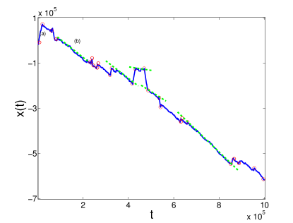
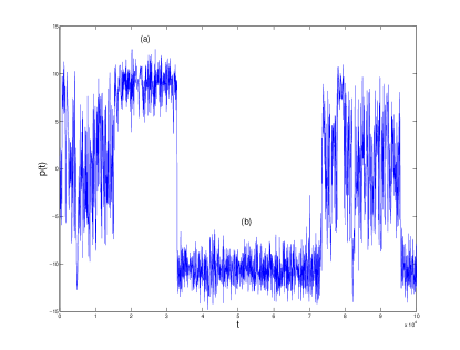
Figure 1: Examples of numerical solutions of the equations of motion. The upper panel depicts the trajectory as a function of time. The dashed lines depict the fitted slopes, corresponding to Eq. (26). The lower panel depicts momentum as a function of time, over a short time scale. Note that (a) and (b) denote the same segments in both figures.

Numerical	Analytic	$P_{n}^{res}$
-10.9149	-10.4243	-8.4742
-0.8898	-0.9152	-0.93063
0.1423	0.1251	0.1266
-9.4296	-10.4642	-8.5484
-0.3535	-0.3577	0.2533
-1.0523	-1.2855	-1.5490
-7.0634	-6.3443	-5.1400

Table 1: Comparison between the numerical value of the slopes of the segments which compose the trajectory presented in Fig.1, and the analytic estimation (26). For comparison, we provide the value of the corresponding $P_{n}^{res}$ for each segment.

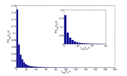
Figure 2: Distribution of the numerical values of the hopping time, $t_{hop}k_{m}\Delta$ (see Eq.(31))

In order to validate the main result of the analytic calculation, we decompose each trajectory of the numerical solution into linear segments as shown in Fig. 1, by using piece-wise linear spline methods ertel1976some . We then fit each segment to a linear function and compare the result to Eq. (26). We find a good agreement between Eq. (26) and the slopes of the linear segments which compose the trajectory, see for example Fig. 1 and table I. We repeat this procedure over many realizations and calculate the relative error between the numerical results and Eq. (26),

$$E_{r}=\left|\frac{p_{stat}-p_{num}}{p_{stat}}\right|.$$ (33)

The distribution of $E_{r}$ is presented in Fig.3.

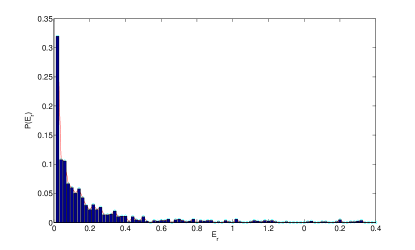
Figure 3: The distribution of the deviation between analytical and numerical results, where $E_{r}$ is given by Eq. (33).

We turn to validate the assumptions of this work. The analysis presented in Sec. IV relies on the assumption that the resonances are separated, (see (14)). We therefore calculate $\eta$ for different resonances for many different realizations. We find that for the studied parameter space, the distribution function of $\eta$ is concentrated around $0.05$, as shown in Fig.4. We can therefore conclude that (14) is satisfied for the parameter space considered in our work.

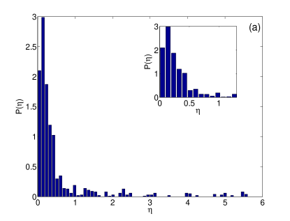
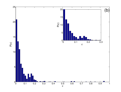
Figure 4: The distributions of the small parameters for the studied systems. (a) The distribution of $\eta$ (b) The distribution of $\varepsilon$. The insets depict the zooms on smaller regimes.

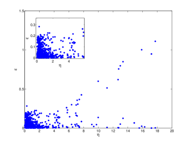
Figure 5: Scatter plot of $\varepsilon$ Vs $\eta$

Figure 6: Distribution of the oscillatory components of momentum, normalized by the characteristic resonance width, $\left|\dot{\xi}/\Delta\right|$.

Figure 4(b) depicts the distribution of $\varepsilon$, the second small parameter in this work, evaluated over many different linear segments. We find that the distribution of $\varepsilon$ is strongly localized near $0$, with a standard deviation which is typically $\mathcal{O}\left(10^{-2}\right)$. This result is consistent with (13) and supports the assumption by which $\varepsilon$ is a small number. Figure 5 depicts a scatter of $\varepsilon$ and $\eta$, which allows a comparison between the relative magnitudes of the small parameter. The scatter of the values of $\eta$ and $\epsilon$ is presented in Fig. 5.

In Sec.III, we have argued that the oscillatory component of the momentum, $\dot{\xi}$ can be taken self consistently to satisfy $\frac{\dot{\xi}}{\Delta}=\mathcal{O}\left(\varepsilon\right)$ and $k_{n}\xi=\mathcal{O}\left(\varepsilon\right)$. We examine this assumption numerically; for each segment, we subtract the calculated slope of the segment and examine the remaining oscillatory component. Fig.6 depicts the probability density function of $\left|\frac{\mbox{$\dot{\xi}$}}{\Delta}\right|$. We find that indeed, the distribution of $\left|\frac{\mbox{$\dot{\xi}$}}{\Delta}\right|$ is strongly localized around an average of $\mathcal{O}\left(10^{-2}\right)$, and is therefore commonly a small parameter. A similar result is found for $k_{n}\xi$.

VI Summary and Discussion

In this we work we calculated the trajectories of classical particles under the action of the potential (3), by estimating the momentum of particles near Chirikov resonances . We found that for short time scales the momentum satisfies Eq. (26), provided the conditions (11), (13) and (14) are satisfied. For these time intervals the position is such that $\xi\left(t\right)$ is of order $\varepsilon$, satisfying (13). If the initial conditions are such that the momentum is near a resonance and $k_{n}\chi\left(0\right)$ is of order $\varepsilon$ the trajectory will remain near a resonance for a time interval of the order $t_{hop}$, otherwise it moves chaotically until it approaches the vicinity of a region in which these conditions are satisfied. It is the main result of this work. This was verified numerically, and in particular, it was demonstrated that there is a wide range of parameters for which Eq. (26) holds. We find that on longer time scales, hopping between Chirikov resonances takes place.

It is interesting to compare our results to previous studies, which examined Eq.(3) in two different limits: extremely small amplitudes and infinite number of overlapping resonances.

In the limit of extremely small amplitudes, $A_{m}\rightarrow 0,\,\forall m$ in Eq.(3), it was predicted zaslavskiui1972stochastic ; Chirikov1979263 that the momentum of a particle will remain localized in phase space. This outcome can be derived from our random walk model by taking the limit of an extremely weak potential (3), $A\rightarrow 0$ and correspondingly, $\eta\rightarrow 0$. In this scenario, no overlap between resonances exists and the hopping is suppressed. As a result, the random walk is replaced with localization in phase space such that $p\left(t\right)=p_{stat}+\mathcal{O}\left(\varepsilon\right)$ remains localized around a single resonance in phase space. This result is reflected in Eq.(31), as in the limit $\eta\rightarrow 0$ and fixed $\varepsilon$, one finds that $t_{hop}\rightarrow\infty$.

Earlier work krivolapov2012transport ; krivolapov2012universality focuses on the behavior of for long time and large $N$. In this limit the number of resonances becomes infinite, and the motion of the particle was found to obey anomalous diffusion in phase space. Since in the large $N$ limit, the resonances become dense in phase space and the rate of hopping between resonances becomes rapid. In this case, the high-rate random walk results in diffusion in phase space Diffusion_and_Reactions_in_Fractals .

The result of the present work can be a starting point of the analysis of the case where there are few weakly overlapping resonances, which is opposite to the one studied in previous work levi-naturephys-2012 . This is a mixed system, where the motion in some parts of the phase space is regular, while in other parts it is chaotic tabor ; book_mechlichtenberglieberman ; RevModPhys.64.795 . The Chirikov theory Chirikov1979263 ; zaslavskiui1972stochastic is not applicable for this case. In addition, the Poincaré-Birkhoff scenario for generation of chaos tabor is not applicable here, since this system is time dependent with incommensurate periods.

The results of this work provide a more complete picture of the dynamics in potentials of the form (1).

We thank Yevgeny Krivolapov (Bar-Lev) for illuminating communications. This work was partly supported by the Israel Science Foundation (ISF - 1028), by the US-Israel Binational Science Foundation (BSF -2010132), by the USA National Science Foundation (NSF DMS 1201394)and by the Shlomo Kaplansky academic chair.

References

- [1] D. S. Lemons and A. Gythiel. Paul langevin’s 1908 paper “On the theory of brownian motion” [“Sur la théorie du mouvement brownien,” c. r. acad. sci. (paris) 146, 530–533 (1908)]. American Journal of Physics, 65(11):1079–1081.
- [2] G. E. Uhlenbeck and L. S. Ornstein. On the theory of the brownian motion. Physical Review, 36(5):823–841, 1930.
- [3] P. A. Sturrock. Stochastic acceleration. Physical Review, 141(1):186–191, 1966.
- [4] B. V. Chirikov. A universal instability of many-dimensional oscillator systems. Physics Reports, 52(5):263 – 379, 1979.
- [5] L. Golubović, S. Feng, and F.-A. Zeng. Classical and quantum superdiffusion in a time-dependent random potential. Physical Review Letters, 67(16):2115–2118, 1991.
- [6] L. Levi, Y. Krivolapov, S. Fishman, and M. Segev. Hyper-transport of light and stochastic acceleration by evolving disorder. Nat Phys, 8(12):912–917, 2012.
- [7] M. Wilkinson. Adiabatic transport of localized electrons. Journal of Physics A: Mathematical and General, 24(11):2615, 1991.
- [8] Y. Krivolapov and S. Fishman. Transport in time-dependent random potentials. Physical Review E, 86(5):051115, 2012.
- [9] Y. Krivolapov and S. Fishman. Universality classes of transport in time-dependent random potentials. Physical Review E, 86(3):030103, 2012.
- [10] V.I. Yukalov, E.P. Yukalova, and V.S. Bagnato. Bose systems in spatially random or time-varying potentials. Laser physics, 19(4):686–699, 2009.
- [11] J. Bourgain. Growth of sobolev norms in linear schrödinger equations with quasi-periodic potential. 204(1):207–247, 1999.
- [12] F. Borgonovi and D. L. Shepelyansky. Particle propagation in a random and quasi-periodic potential. Physica D: Nonlinear Phenomena, 109:24, 1997.
- [13] P. W. Anderson. Absence of diffusion in certain random lattices. Phys. Rev., 109:1492–1505.
- [14] E. Abrahams, P. W. Anderson, D. C. Licciardello, and T. V. Ramakrishnan. Scaling theory of localization: Absence of quantum diffusion in two dimensions. Phys. Rev. Lett., 42:673–676, 1979.
- [15] S. John. Electromagnetic absorption in a disordered medium near a photon mobility edge. Physical Review Letters, 53(22):2169–2172, 1984.
- [16] T. Schwartz, G. Bartal, S. Fishman, and M. Segev. Transport and Anderson localization in disordered two-dimensional photonic lattices. Nature, 446(7131):52–55, 2007.
- [17] J Billy, V Josse, Z Zuo, A Bernard, B Hambrecht, P Lugan, D Clément, L Sanchez-Palencia, P Bouyer, and A Aspect. Direct observation of anderson localization of matter waves in a controlled disorder. Nature, 453(7197):891–894.
- [18] C. Sulem and P.L. Sulem. The Nonlinear Schrödinger Equation: Self-Focusing and Wave Collapse. Number v. 139 in Applied Mathematical Sciences. U.S. Government Printing Office, 1999.
- [19] B.E.A. Saleh and M.C. Teich. Fundamentals of Photonics. Wiley Series in Pure and Applied Optics. Wiley, 2007.
- [20] L. Guidoni, C. Triché, P. Verkerk, and G. Grynberg. Quasiperiodic optical lattices. Phys. Rev. Lett., 79:3363–3366, Nov 1997.
- [21] C. Yuce. Dynamical control in a quasi-periodically modulated optical lattice. Europhysics letters, 103(3):30011, 2013.
- [22] M. Tabor. Chaos and Integrability in Nonlinear Dynamics: An Introduction, volume 86. American Physical Society, 2012.
- [23] A. J. Lichtenberg and M. A. Lieberman. Regular and Chaotic Dynamics (Applied Mathematical Sciences). Springer, 2nd edition, 1992.
- [24] J. D. Meiss. Symplectic maps, variational principles, and transport. Rev. Mod. Phys., 64:795–848, Jul 1992.
- [25] G. M. Zaslavskiĭ and B. V. Chirikov. Stochastic instability of non-linear oscillations. Soviet Physics Uspekhi, 14(5):549–567, 1972.
- [26] M. N. Rosenbluth. Comment on “classical and quantum superdiffusion in a time-dependent random potential”. Phys. Rev. Lett., 69:1831–1831, Sep 1992.
- [27] V. Bezuglyy, B. Mehlig, M. Wilkinson, K Nakamura, and E Arvedson. Generalized ornstein-uhlenbeck processes. Journal of mathematical physics, 47(7):073301, 2006.
- [28] B.V. Chirikov and D.L. Shepelyanskii. Diffusion during multiple passage through a nonlinear resonance. Soviet Physics - Technical Physics, 27(2):156–160, 1982.
- [29] J. E. Ertel and E. B. Fowlkes. Some algorithms for linear spline and piecewise multiple linear regression. Journal of the American Statistical Association, 71(355):640–648, 1976.
- [30] D. Ben-Avraham and S. Havlin. Diffusion and Reactions in Fractals and Disordered Systems. Cambridge University Press, 2000. Cambridge Books Online.