SIMPLIFIED DESCRIPTION OF THE MSSM HIGGS SECTOR

Abstract

In the Minimal Supersymmetric extension of the Standard Model or MSSM, the lighter Higgs boson has a rather large mass, $M_{h}\approx 125$ GeV. Together with the non-observation of superpartners at the LHC, this suggests that the SUSY–breaking scale is rather high, ${M_{S}\raisebox{-3.69899pt}{\leavevmode\nobreak\ \shortstack{$>$ \\ [-0.07cm] $\sim$}}\leavevmode\nobreak\ 1}$ TeV. This implies a dramatic simplification of the MSSM Higgs sector that is summarised here.

1 The post-Higgs boson discovery MSSM Higgs sector

In the MSSM, two Higgs doublets $H_{d}$ and $H_{u}$ are needed to break the electroweak symmetry, leading to three neutral and two charged Higgs states; for a review see Ref.[1]. The tree–level masses of the CP–even $h$ and $H$ bosons depend only on $\tan\beta=v_{d}/v_{u}$, the ratio of vevs of the two doublets and on the pseudoscalar Higgs mass $M_{A}$. Nevertheless, many parameters of the MSSM such as the SUSY scale, taken to be the geometric average of the stop masses $M_{S}\!=\!\sqrt{m_{\tilde{t}_{1}}m_{\tilde{t}_{2}}}$, the higgsino mass $\mu$ and the stop/bottom trilinear couplings $A_{t/b}$ enter $M_{h/H}$ through loop corrections. The CP–even Higgs mass matrix can be written in the basis as:

$${\cal M}_{S}^{2}=M_{Z}^{2}\left(\begin{array}[]{cc}c^{2}_{\beta}&-s_{\beta}c_{\beta}\\ -s_{\beta}c_{\beta}&s^{2}_{\beta}\\ \end{array}\right)+M_{A}^{2}\left(\begin{array}[]{cc}s^{2}_{\beta}&-s_{\beta}c_{\beta}\\ -s_{\beta}c_{\beta}&c^{2}_{\beta}\\ \end{array}\right)+\left(\begin{array}[]{cc}\Delta{\cal M}_{11}^{2}&\Delta{\cal M}_{12}^{2}\\ \Delta{\cal M}_{12}^{2}&\Delta{\cal M}_{22}^{2}\\ \end{array}\right)$$ (7)

where we use the notation $c_{\beta}\!\equiv\!\cos\beta$, $s_{\beta}\!\equiv\!\sin\beta$ and include the radiative corrections into a $2\times 2$ matrix $\Delta{\cal M}_{ij}^{2}$. One can then easily derive the Higgs masses $M_{h,H}$ and the mixing angle $\alpha$ that diagonalizes the $h,H$ system, $h=-\sin\alpha H_{d}^{0}+\cos\alpha H_{u}^{0}$ and $H=\cos\alpha H_{d}^{0}+\sin\alpha H_{u}^{0}$:

$$M_{h/H}^{2} = \frac{1}{2}\big{(}M_{A}^{2}+M_{Z}^{2}+\Delta{\cal M}_{11}^{2}+\Delta{\cal M}_{22}^{2}\mp\sqrt{M_{A}^{4}+M_{Z}^{4}-2M_{A}^{2}M_{Z}^{2}c_{4\beta}+C}\big{)}$$ (8)

$$\tan\alpha = \frac{2\Delta{\cal M}_{12}^{2}-(M_{A}^{2}+M_{Z}^{2})s_{\beta}}{\Delta{\cal M}_{11}^{2}-\Delta{\cal M}_{22}^{2}+(M_{Z}^{2}-M_{A}^{2})c_{2\beta}+\sqrt{M_{A}^{4}+M_{Z}^{4}-2M_{A}^{2}M_{Z}^{2}c_{4\beta}+C}}$$ (9)

$$C=4\Delta{\cal M}_{12}^{4}\!+\!(\Delta{\cal M}_{11}^{2}\!-\!\Delta{\cal M}_{22}^{2})^{2}\!-\!2(M_{A}^{2}\!-\!M_{Z}^{2})(\Delta{\cal M}_{11}^{2}\!-\!\Delta M_{22}^{2})c_{2\beta}\!-\!4(M_{A}^{2}\!+\!M_{Z}^{2})\Delta{\cal M}_{12}^{2}s_{2\beta}$$

In previous works [2, 3], it was pointed out that since the measured value of the $h$ boson mass is high, $M_{h}=125$ GeV, leading to a rather large SUSY-breaking scale [4], $M_{S}\raisebox{-3.69899pt}{\leavevmode\nobreak\ \shortstack{$>$ \\ [-0.07cm] $\sim$}}\leavevmode\nobreak\ 1$ TeV, it implies that the leading radiative corrections are now almost fixed when the constraint $M_{h}=125$ GeV is taken into account. In the $2\times 2$ correction matrix of eq. (7), only the $\Delta{\cal M}^{2}_{22}$ entry which involves the by far leading top/stop corrections proportional to the fourth power of the top Yukawa coupling, is relevant to a good approximation [5]. In this limit $\Delta{\cal M}^{2}_{22}\gg\Delta{\cal M}^{2}_{11},\Delta{\cal M}^{2}_{12}$, one can simply trade $\Delta{\cal M}^{2}_{22}$ for the known $M_{h}$ value:

$$\Delta{\cal M}^{2}_{22}=\frac{M_{h}^{2}(M_{A}^{2}+M_{Z}^{2}-M_{h}^{2})-M_{A}^{2}M_{Z}^{2}c^{2}_{2\beta}}{M_{Z}^{2}c^{2}_{\beta}+M_{A}^{2}s^{2}_{\beta}-M_{h}^{2}}\,.$$ (10)

In this case, called habemus MSSM or hMSSM in Ref.[5], one obtains simple expressions for the mass $M_{H}$ and the angle $\alpha$ in terms of $M_{A},\tan\beta$ and $M_{h}$:

$${\rm hMSSM}:\leavevmode\nobreak\ \leavevmode\nobreak\ \begin{array}[]{l}M_{H}^{2}=\frac{(M_{A}^{2}+M_{Z}^{2}-M_{h}^{2})(M_{Z}^{2}c^{2}_{\beta}+M_{A}^{2}s^{2}_{\beta})-M_{A}^{2}M_{Z}^{2}c^{2}_{2\beta}}{M_{Z}^{2}c^{2}_{\beta}+M_{A}^{2}s^{2}_{\beta}-M_{h}^{2}}\\ \ \ \ \alpha=-\arctan\left(\frac{(M_{Z}^{2}+M_{A}^{2})c_{\beta}s_{\beta}}{M_{Z}^{2}c^{2}_{\beta}+M_{A}^{2}s^{2}_{\beta}-M_{h}^{2}}\right)\,.\end{array}$$ (13)

Concerning the charged Higgs boson, the quantum corrections to its mass are much smaller for large $M_{A}$, and one can write to a good approximation, $M^{2}_{H^{\pm}}\simeq M_{A}^{2}+M_{W}^{2}$.

This approach allows to disregard the radiative corrections in the MSSM Higgs sector and their complicated dependence on all the MSSM parameters. This considerably simplifies the phenomenological studies in the MSSM Higgs sector which up to now do not use the constraint $M_{h}=125$ GeV as an input as it should be, and rely either on benchmark scenarios in which most of the MSSM parameters are fixed or refuge to large scans over the parameter space.

2 Fit of the SM Higgs couplings

In the MSSM, the couplings of the lighter $h$ state to gauge bosons and fermions, normalized to their SM values read:

$$c_{V}^{0}\!=\!\sin(\beta\!-\!\alpha)\ ,\ \ c_{t}^{0}\!=\!\frac{\cos\alpha}{\sin\beta}\ ,\ \ c_{b}^{0}\!=\!-\frac{\sin\alpha}{\cos\beta}\,.$$ (14)

They depend on the tree–level inputs $\tan\beta$ and $M_{A}$ but also on the full MSSM spectrum because of the quantum corrections that enter the angle $\alpha$ as in the case of the Higgs masses. As discussed earlier, knowing $\tan\beta$ and $M_{A}$ and fixing $M_{h}$ to its measured value, the couplings can be determined. Nevertheless, this applies only for the radiative corrections to the Higgs masses. In addition, there exists direct radiative corrections to the Higgs couplings different from the ones of the mass matrix in eq. (7) and which will complicate the situation.

If the $h$ coupling to the bottom and top quarks could be significantly modified (by stop loops in the production process $gg\to h$ in the former and by the $\Delta_{b}$ corrections in the latter cases; see Ref.[5]), $c_{t,b}^{0}\to c_{t,b}$, the couplings to $\tau$ leptons and $c$ quarks do not receive substantial direct corrections and one still has $c_{c,\tau}\approx c_{t,b}^{0}$. Consequently, because of the direct radiative corrections, the Higgs couplings cannot be described by only $\beta$ and $\alpha$ as in eq. (14). To characterize the Higgs particle at the LHC, it was advocated [5] that three independent $h$ couplings should be considered, namely $c_{t}$, $c_{b}$ and $c_{V}=c_{V}^{0}$. Thus, one can define the following effective Lagrangian:

$${\cal L}_{h} \!=\! c_{V}g_{hVV}hV_{\mu}^{+}V^{-\mu}+c_{t}y_{t}h\bar{t}_{L}t_{R}\!-\!c_{t}y_{c}h\bar{c}_{L}c_{R}\!-\!c_{b}y_{b}h\bar{b}_{L}b_{R}\!-\!c_{b}y_{\tau}h\bar{\tau}_{L}\tau_{R}\!+\!{\rm h.c.}$$ (15)

where $y_{t,c,b,\tau}=m_{t,c,b,\tau}/v$ are the Yukawa couplings of the heavy SM fermions, $g_{hVV}\!=\!2M^{2}_{V}/v$ the $hVV$ couplings with $V\!=\!W,Z$. Following an earlier analysis performed in Ref.[6] where details can be found, a three–dimensional fit of the $\sqrt{s}=7+$8 TeV ATLAS and CMS Higgs data has been performed and the result in the space $[c_{t},c_{b},c_{V}]$ is shown on the left-hand side of Fig. 1. The obtained best-fit values for the Higgs couplings are: $c_{t}=0.89$, $c_{b}=1.0$ and $c_{V}=1.02$.

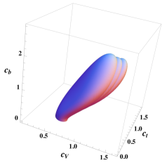
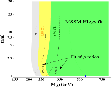
Figure 1: Left: best-fit regions at 99%CL for the Higgs signal strengths in the three dimensional space $[c_{t},c_{b},c_{V}]$ [5]. Right: best-fit regions for the signal strengths and their ratios in the plane $[\tan\beta,M_{A}]$; the best point is in blue [5].

In cases where the direct corrections are not quantitatively significant one can reduce the number of effective parameters down to two using the MSSM relations of eq. (14). Using the formulae of eq. (13) for the mixing angle and the $M_{h}\!\approx 125$ GeV value as an input, one can perform a fit in the $[\tan\beta,M_{A}]$ plane as shown on the right-hand side of Fig. 1. It illustrates the 68%, 95% and 99%CL contours obtained from fitting the signal strengths and their ratios. The best-fit point is realized for the values $\tan\beta\!=\!1$ and $M_{A}\!=\!557\;{\rm GeV}$, which translates into $M_{H}=580$ GeV, $M_{H^{\pm}}=563$ GeV and $\alpha=-0.837\leavevmode\nobreak\ {\rm rad}$. Such a low $\tan\beta$ point implies an extremely large SUSY scale value, $M_{S}={\cal O}(100)$ TeV to accommodate a $125$ GeV Higgs boson. Notice, that the $\chi^{2}$ value is relatively flat all over the $1\sigma$ region and, thus, larger $\tan\beta$ values could also be appropriate, hence allowing for not too large SUSY scale values. Nevertheless, one obtains that the pseudoscalar should verify $M_{A}\raisebox{-3.69899pt}{\leavevmode\nobreak\ \shortstack{$>$ \\ [-0.07cm] $\sim$}}\leavevmode\nobreak\ 200$ GeV in all cases.

3 Heavy scalar searches

In our quite “model–independent” approach, defined in eq. (13), we make no restriction on the SUSY scale which can be at any value, even quite high. It allows to reopen the small $\tan\beta$ region, $\tan\beta\!\raisebox{-3.69899pt}{\leavevmode\nobreak\ \shortstack{$<$ \\ [-0.07cm] $\sim$}}\leavevmode\nobreak\ \!3$, that was long thought to be excluded from the negative search of a SM–like scalar boson at LEP which set the limit $M_{h}\!\raisebox{-3.69899pt}{\leavevmode\nobreak\ \shortstack{$>$ \\ [-0.07cm] $\sim$}}\leavevmode\nobreak\ \!114$ GeV, but assuming a setting with $M_{S}\!\raisebox{-3.69899pt}{\leavevmode\nobreak\ \shortstack{$<$ \\ [-0.07cm] $\sim$}}\leavevmode\nobreak\ \!1$ TeV. If $M_{S}$ is large enough as indicated by present data (see Ref.[4] for example), low $\tan\beta$ values would still be allowed. In the left-hand side of Fig. 2, we display the contours in the plane $[\tan\beta,M_{S}]$ for mass values in the window $M_{h}=120$–132 GeV of the observed Higgs state.

The contour corresponding to the LEP2 limit $M_{h}=114$ GeV indicates that $\tan\beta\approx 1$ is still viable provided that $M_{S}\raisebox{-3.69899pt}{\leavevmode\nobreak\ \shortstack{$>$ \\ [-0.07cm] $\sim$}}\leavevmode\nobreak\ 20$ TeV. The present value $M_{h}=125$ sets stronger constraints: for example, while one can accommodate a scale $M_{S}\approx 1$ TeV with $\tan\beta\approx 5$, a large scale $M_{S}\approx 20$ TeV is required to obtain $\tan\beta\approx 2$. Let us discuss the implications for heavy Higgs searches.

The most promising process to look for the heavier MSSM Higgs scalars is by far $pp\!\to\!gg\!+\!bb\!\to\!H/A\!\to\!\tau\tau$. Searches for this channel have been performed by ATLAS [7] with $\approx 5$ fb^-1 data at the 7 TeV run and by CMS [8] with $\approx 5+20$ fb^-1 data at the 7 TeV and 8 TeV runs. Upper limits on the production cross section times decay branching ratio have been set and they can be turned into constraints on the MSSM parameter space. The sensitivity of the CMS $pp\to h,H,A\to\tau\tau$ analysis in the plane $[\tan\beta,M_{A}]$ using 25 fb^-1 of data can be found in Ref.[8]. The excluded region obtained from the observed limit at the 95%CL is extremely restrictive and for $M_{A}\approx 250$ GeV the high $\tan\beta\raisebox{-3.69899pt}{\leavevmode\nobreak\ \shortstack{$>$ \\ [-0.07cm] $\sim$}}\leavevmode\nobreak\ 10$ region is entirely excluded and one is even sensitive to large values $M_{A}\approx 800$ GeV for $\tan\beta\raisebox{-3.69899pt}{\leavevmode\nobreak\ \shortstack{$>$ \\ [-0.07cm] $\sim$}}\leavevmode\nobreak\ 45$.

Nevertheless, there is a caveat to this exclusion limit because the constraint applies for a particular benchmark, the maximal mixing scenario with $X_{t}/M_{S}=\sqrt{6}$, assuming $M_{S}=1$ TeV. In fact this exclusion limit is valid in far more situations than the “MSSM $M_{h}^{\rm max}$ scenario” and it should be extended to the low $\tan\beta$ regime which, in the chosen scenario with $M_{S}=1$ TeV, is excluded by the LEP2 limit on the lighter $h$ mass but is resurrected if the SUSY scale is kept as a free parameter. Reopening the low $\tan\beta$ region allows to hunt for the heavier scalar bosons in various interesting processes at the LHC. Heavier CP–even $H$ decays into massive gauge bosons $H\to WW,ZZ$ and lighter Higgs bosons $H\to hh$, CP–odd scalar decays into a vector and a Higgs boson, $A\to hZ$, CP–even and CP–odd scalar decays into top quarks, $H/A\to t\bar{t}$, and the charged scalar decays into a gauge boson and a Higgs boson, $H^{\pm}\to Wh$.

A preliminary study of these processes has been performed [3] relying on the searches for the SM Higgs boson or other heavy resonances made by the ATLAS and CMS collaborations. The results which are shown on the left-hand of Fig. 2 are interesting since these searches cover a large part of the parameter space of the MSSM Higgs sector in a model–independent way, i.e. without the need to precise the SUSY particle spectrum that appear in the quantum corrections. More especially, the channels $H\to VV$ and $H/A\to t\bar{t}$ are very constraining as they probe the entire low $\tan\beta$ area up to $M_{A}\approx 600$ GeV. Notice that $A\to hZ$ and $H\to hh$ could also be seen at the current LHC in small parts of the MSSM parameter space.

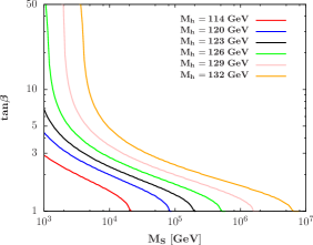
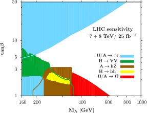
Figure 2: Left: contours for fixed values $M_{h}=120$–132 GeV in the $[\tan\beta,M_{S}]$ plane in the decoupling limit $M_{A}\gg M_{Z}$; the “LEP2 contour” for $M_{h}=114$ GeV is shown in red. Right: the estimated sensitivities [3] in the various search channels for the heavier MSSM Higgs bosons in the $[\tan\beta,M_{A}]$ plane: $H/A\!\to\!\tau\tau$, $H\!\to\!WW\!+\!ZZ$, $H/A\!\to\!t\bar{t}$, $A\!\to\!hZ$ and $H\!\to\!hh$. Taken from Ref.[3].

4 Summary

We have discussed a simplified framework that describes the MSSM Higgs sector after the discovery of the lighter $h$ boson. Including the constraint $M_{h}\!=\!125$ GeV, it can be again parameterized by the two inputs $\tan\beta$ and $M_{A}$ as at tree-level, irrespective of the SUSY parameters that enter the radiative corrections such as the SUSY scale $M_{S}$. Allowing large $M_{S}$ values reopens the low $\tan\beta$ region which can be probed in many interesting processes at the LHC. This is the case of e.g. the processes $gg\to H/A\to t\bar{t}$ which need further studies [9].

References

References

• [1] A. Djouadi, Phys. Rept. 459, 1 (2008); Phys. Rept. 457, 1 (2008); arXiv:1311.0720.
• [2] L. Maiani, A. Polosa and V. Riquer, New J. Phys. 14, 073029 (2012);
Phys. Lett. B 718, 465 (2012); Phys. Lett. B 724, 274 (2013).
• [3] A. Djouadi and J. Quevillon, JHEP 10, 028 (2013).
• [4] A. Arbey et al, Phys. Lett. B 708, 162 (2012); JHEP 09, 107 (2012).
• [5] A. Djouadi, L. Maiani et al, Eur.Phys.J. C 73, 2650 (2013).
• [6] A. Djouadi and G. Moreau, Eur.Phys.J. C 73, 2512 (2013).
• [7] ATLAS Collaboration, JHEP 1302, 095 (2013).
• [8] CMS Collaboration, CMS-PAS-HIG-13-021.
• [9] J. Quevillon et al, in preparation.