Optimal stopping under model uncertainty: randomized stopping times approach
Denis Belomestnylabel=e1]denis.belomestny@uni-due.de
[Volker Krätschmerlabel=e2]volker.kraetschmer@uni-due.de
[
Duisburg-Essen University
Duisburg-Essen University
Faculty of Mathematics
Thea-Leymann-Str. 9
D-45127 Essen
Germany
E-mail: e2
Abstract
In this work we consider optimal stopping problems with conditional convex risk measures
of the form
where is a lower semicontinuous convex mapping and stands for the set of all probability measures which are absolutely continuous w.r.t. a given measure and on Here the model uncertainty risk depends on a (random) divergence
measuring the distance between a hypothetical probability measure we are uncertain about and a reference one at time
Let be an adapted nonnegative, right-continuous stochastic process fulfilling some proper integrability condition and let be the set of stopping times on , then without assuming any kind of time-consistency for the family we derive a novel representation
which makes the application of the standard dynamic programming based approaches possible.
In particular, we generalize the additive dual representation of Rogers, [38] to the case of optimal stopping under uncertainty. Finally, we develop several Monte Carlo algorithms and illustrate their power for optimal stopping under Average Value at Risk.
60G40,
60G40,
91G80,
Optimized certainty equivalents,
optimal stopping,
primal representation,
additive dual representation,
randomized stopping times,
thin sets,
keywords:
[class=MSC]
keywords:
\arxiv
arXiv:0000.0000
\startlocaldefs\endlocaldefs
and
T1This research was partially supported by the Deutsche
Forschungsgemeinschaft through the SPP 1324 “Mathematical methods for extracting quantifiable information from complex systems” and by
Laboratory for Structural Methods of Data Analysis in Predictive Modeling, MIPT, RF government grant, ag. 11.G34.31.0073.
1 Introduction
In this paper we study the optimal stopping problems in an uncertain environment.
The classical solution to the optimal stopping problems based on the dynamic programming principle assumes that there is a unique subjective prior distribution driving the reward process.
However, for example, in incomplete financial markets, we have to deal with multiple equivalent martingale measures not being sure which one underlies the market. In fact under the presence of the multiple possible distributions, a solution of the optimal stopping problem by maximization with respect to some subjective prior cannot be reliable. Instead, it is reasonable to view the multitude of possible distributions as a kind of model uncertainty risk which should be taken into account while formulating an optimal stopping problem. Here one may draw on concepts from the theory of risk measures. As the established generic notion for static risk assessment at present time , convex risk measures are specific functionals on vector spaces of random variables viewed as financial risks (see [27] and [28]). They typically have the following type of robust representation
(1.1)
where denotes the set of probability measures which are absolutely continuous w.r.t. a given reference probability measure and is some penalty function (see e.g. [15] and [25]). In this way, model uncertainty is incorporated, as no specific probability measure is assumed. Moreover, the penalty function scales the plausibility of models.
Turning over from static to dynamic risk assessment, convex risk measures have been extended to the concept of conditional convex risk measures at a future time which are specific functions on the space of financial risks with random outcomes (see [9], [19] and [16]). Under some regularity conditions, they have a robust representation of the form (see e.g. [26], [18] or [25, Chap. 11])
(1.2)
where is a (random) penalty function and consists of all with As in (1.1), the robust representation (1.2) mirrors the model uncertainty, but now at a future time
In recent years the optimal stopping with families of conditional convex risk measures was subject of several studies. For example, the works
[36] and [32] are settled within a time-discrete framework, where in addition the latter one provides some dual representations extending the well-known ones from the classical optimal stopping. Optimal stopping in continuous time was considered in [5], [6], [7], [14]. All these contributions restrict their analysis to the families satisfying the property of time consistency, sometimes also called recursiveness, defined to mean
Hence the results of the above papers can not be, for example, used to solve optimal stopping problems under such very popular convex risk measure as Average Value at Risk.
The only paper which tackled the case of non time-consistent families of conditional convex risk measures so far is [40], where the authors considered the so-called distorted mean payoff functionals.
However, the analysis of [40] excludes the case of Average Value at Risk as well. Moreover, the class of processes to be stopped is limited to the functions of a one-dimensional geometric Brownian motion. The main probabilistic tool used in [40] is the Skorokhod embedding.
In this paper we consider a rather general class of conditional convex risk measures having representation (1.2)
with
for some lower semicontinuous convex mapping The related class of risk measures known as the class of divergence risk measures or optimized certainty equivalents was first introduced in [10],
[11]. Any divergence risk measure has the representation
with
(cf. [10], [11], [17], or Appendix A).
Here we study the problem of optimally stopping the reward process where is an adapted nonnegative, right-continuous stochastic process with satisfying some suitable integrability condition. We do not assume any time-consistency for the family and basically impose no further restrictions on . Our main result is the representation
(1.3)
which allows one to apply the well known methods from the theory of ordinary optimal stopping problems. In particular, we derive the so-called additive dual representation of the form:
(1.4)
where is the class of adapted martingales vanishing at time 0. This dual representation generalizes the well-known dual representation of Rogers, [38].
The representation (1.4) together with (1.3) can be used to efficiently construct lower and upper bounds for the optimal value (1.3) by Monte Carlo.
The paper is organised as follows. In Section 2 we introduce notation and set up the optimal stopping problem. The main results are presented in Section 3 where in particular a criterion ensuring the existence of a saddle-point in (1.3) is formulated. Section 4 contains some discussion on the main results and on their relation to the previous literature. A Monte Carlo algorithm for computing lower and upper bounds for the value function is formulated in Section 5, where also an example of optimal stopping under Average Value at Risk is numerically analized.
The crucial idea to derive representation (1.3) is to consider the optimal stopping problem
where denotes the set of all randomized stopping times on It will be studied in Section 6, where in particular it will turn out that this optimal stopping problem has the same optimal value as the originial one. Finally, the proofs are collected in Section 7.
2 The set-up
Let be a probability space and denote by the class of all finitely-valued random variables (modulo the -a.s. equivalence). Let be a Young function, i.e., a left-continuous, nondecreasing convex function such that and . The Orlicz space associated with is defined as
It is a Banach space when endowed with the Luxemburg norm
The Orlicz heart is
For example, if for some then is the usual space. In this case where
stands for norm. If takes the value , then and is defined to consist of all essentially bounded random variables. By Jensen inequality, we always have In the case of finite we see that is a linear subspace of which is dense w.r.t. (see Theorem 2.1.14 in [21]).
Let and let be a filtered probability space, where
is a right-continuous filtration with containing only the sets with probability or as well as all the null sets of . Furthermore, consider a lower semicontinuous convex mapping satisfying
for some and
Its Fenchel-Legendre transform
is a finite nondecreasing convex function whose restriction to
is a finite Young function (cf. Lemma A.1 in Appendix A). We shall use
to denote the Orlicz heart w.r.t. Then we can define a conditional convex risk measure via
for all where denotes the set of all probability measures which are absolutely continuous w.r.t. such that is integrable and on Note that
is integrable for every and any
due to the Young’s inequality. Consider now a right-continuous nonnegative stochastic process adapted to Furthermore, let contain all finite stoping times w.r.t. The main object of our study is the following optimal stopping problem
(2.1)
If we set for and
otherwise, we end up with the classical stopping problem
(2.2)
It is well known that the optimal value of the problem (2.2) may be viewed as a risk neutral price of the American option with the discounted payoff at time However, in face of incompleteness, it seems to be not appropriate to assume the uniqueness of the risk neutral measure. Instead, the uncertainty about the stochastic process driving the payoff should be taken into account. Considering the optimal value of the problem (2.1) as an alternative pricing rule, model uncertainty risk is incorporated by taking the supremum over where the penalty function is used to assess the plausibility of possible models. The more plausible is the model, the lower is the value of the penalty function.
Example 2.1.
Let us illustrate our setup in the case of the so called Average Value at Risk risk measure. The Average Value at Risk risk measure at level is defined as the following functional:
where and denotes the left-continuous quantile function of the distribution function of defined by for . Note that for any Moreover, it is well known that
where is the Young function defined by
for and otherwise (cf. [25, Theorem 4.52] and [30]). Observe that the set consists of all probability measures on with
a.s.. Hence the optimal stopping problem
(2.1) reads as follows
(2.3)
The family of conditional convex risk measure associated with
is also known as the conditional AV@R at level
(cf. [25, Definition 11.8]).
Example 2.2.
Let us consider, for any the continuous convex mapping defined by for and The Fenchel-Legendre transform of is given by
for In view of Lemma A.1 (cf. Appendix A) the corresponding risk measure
has the representation
(2.4)
for This is the well-known entropic risk measure. Optimal stopping with the entropic risk measures is easy to handle, since it can be reduced to the standard optimal stopping problems via
(2.5)
Example 2.3.
Set for any then the set contains all probability measures on with
and
3 Main results
Let denote the topological interior of the effective domain of the mapping We shall assume to be a lower semicontinuous convex function satisfying
(3.1)
3.1 Primal representation
The following theorem is our main result.
Theorem 3.1.
Let be atomless with countably generated for every Furthermore, let (3.1) be fulfilled, and let then
Remark 3.2.
The functional
is known as the optimized certainty equivalent w.r.t. (cf.
[10],[11]). Thus the relationship
(3.2)
may also be viewed as a representation result for optimal stopping with optimized certainty equivalents.
Let us illustrate Theorem 3.1 for the case with some The Young function satisfies the conditions of Theorem 3.1 if and only if The Fenchel-Legendre transform of is given by
and it fullfills the inequality for Then, as an immediate consequence of Theorem 3.1, we obtain the following primal representation for the optimal stopping problem
(2.3).
Corollary 3.3.
Let be atomless with countably generated for every If
then it holds for
Let us now consider the case for some This mapping meets all requirements of Theorem 3.1, and Then by Theorem 3.1, we have the following primal representation of the corresponding optimal stopping problem.
Corollary 3.4.
Let be atomless with countably generated for every If
for some
then
3.2 The existence of solutions
A natural question is whether we can find a real number and a -stopping time which solve (3.2). We may give a fairly general answer within the context of discrete time optimal stopping problems. In order to be more precise, let denote all stopping times from with values in where is any finite subset of containing Consider now the stopping problem
(3.3)
Turning over to the filtration defined by
with we see that
with describes some adapted process. Hence we can apply Theorem 3.1 to get
(3.4)
In this section we want to find conditions which guarantee the existence of a saddle point for the optimization problems
(3.5)
and
(3.6)
To this end, we shall borrow some arguments from the theory of Lyapunoff’s theorem for infinite-dimensional vector measures. A central concept in this context is the notion of thin subsets of integrable mappings. So let us first recall it. For a fixed probability space a subset is called thin if for any with there is some
nonzero vanishing outside and satisfying for every (cf. [31], or [1]). Best known examples are finite subsets of or
finite-dimensional linear subspaces of if
is atomless (cf. [31], or [1]).
Proposition 3.5.
Let the assumptions of Theorem 3.1
be fulfilled, and let
with
Moreover, let be a thin subset of for with and
Then there are and satisfying
In particular, it holds
for any and
The proof of Proposition 3.5 can be found in Section 7.5.
Example 3.6.
Let the mapping be defined by for some Obviously, is convex, nondecreasing, and satisfies as well as Hence defines a lower semicontinuous convex function which satisfies (3.1), and whose Fenchel-Legendre transform coincides with since is continuous.
Moreover, for any such that and the set is contained in the finite-dimensional linear subspace of spanned by the sequence of r. v.
where by definition
As a result,
is a thin subset of in the case of atomless (cf. e.g. [1, Proposition 2.6]).
3.3 Additive dual representation
In this section we generalize the celebrated additive dual representation for optimal stopping problems (see [38]) to the case of optimal stopping under uncertainty. The result in [38] is formulated in terms of martingales with satisfying The set of all such adapted martingales will be denoted by
Theorem 3.7.
Let
be the Snell envelope of an integrable right-continuous stochastic process adapted to
If for some then
where the infimum is attained for with being the martingale part of the Doob-Meyer decomposition of Even more it holds
Remark 3.8.
By inspection of the proof of Theorem 2.1 in [38], one can see that the assumption for some is only used to guarantee the existence of the Doob-Meyer decomposition of the Snell envelope Therefore this assumption may be relaxed, if we consider discrete time optimal stopping problems on the set for some finite containing In this case, the Doob-Meyer decomposition always exists if is integrable, and Theorem 3.7 holds with replaced by and replaced by (see also
[32, Theorem 5.5]).
Theorem 3.1 allows us to extend the additive dual representation to the case of stopping problems
(2.1). We shall use the following notation. For a fixed and we shall denote by the Snell-envelope w.r.t. to defined via
The application of Theorem 3.1 together with Theorem 3.7 provides us with the following additive dual representation of the stopping problem (2.1).
Theorem 3.9.
Under assumptions on and of Theorem 3.1 and under the condition for some and any the following dual representation holds
Here
stands for the martingale part of the Doob-Meyer decomposition of the Snell-envelope
Remark 3.10.
Under the assumptions of Theorem 3.1, we have that Furthermore, is convex and nondecreasing with (see Lemma A.1 in Appendix A) so that for any
where denotes the right-sided derivative of Using the monotonicity of again, we conclude that
for all and Hence the application of Theorem 3.9 to (3.3) is already possible under the assumptions of Theorem 3.1.
The dual representation for the optimal stopping problem under Average Value at Risk reads as follows.
Corollary 3.11.
Let the assumptions on and be as in Theorem 3.1. If
for some then it holds
-a.s.
(3.7)
Here
denotes the martingale part of the Doob-Meyer decomposition of
the Snell-envelope
Remark 3.12.
Let us consider a discrete time optimal stopping problem for some finite with In view of Remark 3.10, the assumptions of Theorem 3.1 are already sufficient to obtain the dual representation (3.7) with replaced by and replaced by
were studied, where for any the functional maps a linear subspace
of the space into and satisfies for a.s.. In fact there is a one-to-one correspondence between conditional convex risk measures and dynamic utility functionals satisfying the following two properties:
•
conditional translation invariance:
for
and
•
conditional concavity:
for
and with
More precisely, any conditionally translation invariant and conditionally concave dynamic utility functional defines a family of conditional convex risk measures via and vice versa. The results of [32] essentially rely on the following additional assumptions
•
regularity:
for and
•
recursiveness:
for
Recursiveness is often also referred to as time consistency. Obviously, the dynamic utility functional defined by satisfies the regularity and the conditional translation invariance, but it fails to be recursive (cf. [25, Example, 11.13]). Even worse, according to Theorem 1.10 in [34] for any there is in general no regular conditionally translation invariant and recursive dynamic utility functional such that This means that we can not in general reduce the stopping problem (2.3) to
the stopping problem (4.1) with a regular, conditionally translation invariant and recursive dynamic utility functional . Note that this conclusion can be drawn from Theorem 1.10 of [34], because is law-invariant, i.e.,
for identically distributed and , and satisfies the properties as well as
for any and with
The stopping problem (2.3) may also be viewed as a special case of the following stopping problem:
(4.2)
where is a so-called distortion function, i.e., is nondecreasing and satisfies Indeed, if for
the distortion function is defined by
then the stopping problems (2.3) and (4.2) coincide. Recalling Theorem 1.10 of [34] again, we see that the stopping problem
(4.2) is not in general representable in the form (4.1) with some regular, conditionally translation invariant and recursive dynamic utility functional.
The stopping problem (4.2) was recently considered by [40]. However, the analysis in [40] relies on some additional assumptions. First of all, the authors allow for all finite stopping times w.r.t. to some filtered probability space instead of restricting to those which are bounded by a fixed number. Secondly, they assume a special structure for the process namely it is supposed that for an absolutely continuous nonnegative function on and for a one-dimensional geometric Brownian motion . Thirdly, the authors focus on strictly increasing absolutely continuous distortion functions so that their analysis does not cover the case of Average Value at Risk. More precisely,
in [40] the optimal stopping problems of the form
(4.3)
are studied, where denotes the set of all finite stopping times. A crucial step in the authors’ argumentation is the reformulation of the optimal stopping problem (4.3) as
where and are derivatives of and respectively, and denotes the set of all distribution functions with a nonnegative support such that
The main idea of the approach in [40] is that any such distribution function may be described as the distribution function of for some finite stopping time and this makes the application of the Skorokhod embedding technique possible. Hence, the results essentially rely on the special structure of the stochastic process and seem to be not extendable to stochastic processes of the form where is a multivariate Markov process. Moreover, it remains unclear whether the analysis of [40] can be carried over to the case of bounded stopping times, as the Skorokhod embedding can not be applied to the general sets of stopping times (see e.g. [3]).
5 Numerical example
In this section we illustrate how our results can be used to price Bermudan-type options in uncertain environment.
Specifically, we consider the model with identically distributed assets, where each underlying has dividend yield .
The dynamic of assets is given by
(5.1)
where , are independent one-dimensional Brownian
motions and are constants. At any time the holder of the option may exercise it and
receive the payoff
If we are uncertain about our modelling assumption and if the Average Value at Risk is used to measure the risk related to this uncertainty, then the risk-adjusted
price of the option is given by
(5.2)
where consists of all probability measures on with
(5.3)
If we restrict our attention to the class of generalised Black Scholes models of the type
with adapted processes and independent Brownian motions then
Due to Corollary 3.3, one can use the standard methods based on dynamic programming principle to
solve (5.2) and stands for a set of stopping times with values in
Indeed, for any fixed the optimal value of the stopping problem
can be, for example, numerically approximated via the well known regression methods like Longstaff-Schwartz method. In this way one can get a (suboptimal) stopping rule
where are continuation values estimates. Then
(5.4)
is a low-biased estimate for . Note that the infimum in (5.4) can be easily computed using a simple search algorithm. An upper-biased estimate can be constructed using the well known Andersen-Broadie dual approach (see [2]). For any fixed this approach would give us a discrete time martingale which in turn can be used to build an upper-biased estimate via the representation (3.7):
(5.5)
Note that (5.5) remains upper biased even if we replace the infimum of the objective function in (5.5) by its value at a fixed point
In Table 1 we present the bounds and together with their standard deviations for different values of As to implementation details, we used basis functions for regression (see [2]) and training paths to compute
In the dual approach of Andersen and Broadie, inner simulations were done to approximate In both cases we simulated testing paths to compute the final estimates.
For comparison let us consider a problem of pricing the above Bermudan option under entropic risk measure (2.4). Due to (2.5), we need to solve the optimal stopping problem
The latter problem can be solved via the standard dynamic programming combined with regression as described
above. In Table 2 the upper and lower MC bounds for are presented for different values of the parameter Unfortunately for larger values of the corresponding MC estimates become unstable due to the presence of exponent in (2.5).
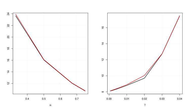
In Figure 1 the lower bounds for AV@R and the entropic risk measure are shown graphically.
As can be seen the quality of upper and lower bounds are quite similar. However due to above mentioned instability, AV@R should be preferred under higher uncertainty.
Figure 1: Lower and upper bounds for Bermudan option prices under AV@R (left) and entropic risk (right) measures.
Table 1: Bounds (with standard deviations) for -dimensional Bermudan max-call with parameters , under AV@R at level
Lower bound
Upper bound
0.33
23.64(0.026)
23.92(0.108)
0.50
16.06(0.019)
16.12(0.045)
0.67
12.05(0.014)
12.09(0.034)
0.75
10.71(0.013)
10.75(0.030)
Table 2: Bounds (with standard deviations) for -dimensional Bermudan max-call with parameters , under entropic risk measure with parameter
Lower bound
Upper bound
0.0025
8.218979 (0.011)
8.262082 (0.029)
0.005
8.399141 (0.015)
8.454748 (0.032)
0.01
8.797425 (0.017)
8.888961 (0.041)
0.02
9.698094 (0.020)
10.03958 (0.058)
0.03
12.72327 (0.020)
12.74784 (0.072)
0.04
17.47090 (0.022)
17.50481 (0.095)
6 The optimal stopping problem with randomized stopping times
In order to prove Theorem 3.1 we shall proceed as follows.
First, by Lemma A.1 (cf. Appendix A), we obtain immediately
(6.1)
The proof of Theorem 3.1 would be completed, if we can show that
(6.2)
Using Fubini’s theorem, we obtain for any and every
where stands for the distribution function of and denotes the right-sided derivative of the convex function In the same way we may also find
Hence the property for yields
(6.3)
for and Since the set of distribution functions
of is not, in general, a convex subset of the set of distribution functions on we can not apply the known minimax results. The idea is to first establish (6.2) for the larger class of randomized stopping times, and then to show that the optimal value coincides with the optimal value
Let us recall the notion of randomized stopping times. By definition
(see e.g. [20]), a randomized stopping time w.r.t. is
a mapping which is nondecreasing and left-continuous in the second component such that is a stopping time w.r.t. for any Notice that any randomized stopping time is also an ordinary stopping time w.r.t. the enlarged filtered probability space
Here
denotes the uniform distribution on defined on the usual Borel algebra on We shall call a randomized stopping time to be degenerated if is constant for every There is an obvious one-to-one correspondence between stopping times and degenerated randomized stopping times.
Consider the stochastic process defined by
which is adapted w.r.t. the enlarged filtered probability space.
Denoting by the set of all randomized stopping times we shall study the following new stopping problem
(6.4)
Obviously, is valid for every stopping time where is the corresponding degenerated randomized stopping time such that Thus, in general the optimal value of the stopping problem (6.4) is at least as large as the one of the original stopping problem
(2.1) due to (6.1). One reason to consider the new stopping problem (6.4) is that it has a solution under fairly general conditions.
Proposition 6.1.
Let be quasi-left-continuous, defined to mean a.s. whenever is a sequence in satisfying for some . If is countably generated, then there exists a randomized stopping time such that
Proposition will be proved in Section 7.1.
Moreover
the following important minimax result for the stopping problem
(6.4) holds.
Moreover, if is quasi-left-continuous and if is countably generated, then there exist and such that
for and
The proof of Proposition 6.2 can be found in Section 7.2.
In the next step we shall provide conditions ensuring that the stopping problems
(2.1) and (6.4) have the same optimal value.
Proposition 6.3.
Let be atomless with countably generated for every If (3.1) is fulfilled, and if belongs to then
The proof of Proposition 6.3 is delegated to Section 7.3.
7 Proofs
We shall start with some preparations which also will turn out to be useful later on. Let us recall (cf. [20]) that every
induces a
stochastic kernel
with being the distribution of under for any Here stands for the usual Borel algebra on This stochastic kernel has the following properties:
The associated stochastic kernel is useful to characterize the distribution function of
Lemma 7.1.
For any with associated stochastic kernel the distribution function of may be represented in the following way
Proof
Let and let us fix Then
holds (cf. [20, Theorem 4.5]), where the last equation on the right hand side is due to Fubini-Tonelli theorem. Then by definition of we obtain for every
This completes the proof.
Following a suggestion by one referee we placed the proof of Proposition 6.1 in front of that of Proposition 6.2.
Let us introduce the filtered probability space defined by
We shall denote by the set of randomized stopping times according to Furthermore, we may extend the processes
and to right-continuous processes
and in the following way
Recall that we may equip with the so called Baxter-Chacon topology which is compact in general, and even metrizable within our setting because is assumed to be countably generated (cf. Theorem 1.5 in [4] and discussion afterwards).
Next, consider the mapping
By assumption on , the processes and are quasi-left-continuous. Moreover, is continuous due to Lemma A.1, (i) in Appendix A, so that is a quasi-left-continuous and right-continuous adapted process. Hence in view of [20, Theorem 4.7], the mapping is continuous w.r.t. the Baxter-Chacon topology for every and thus
is upper semicontinuous w.r.t. the Baxter-Chacon topology. Then by compactness of the Baxter-Chacon topology, we may find some randomized stopping time
such that
This completes the proof because
and
belongs to for every
Since is assumed to belong to the mapping
is finite and convex, and thus continuous. Moreover, by Lemma A.1 (cf. Appendix A)
Hence for some Thus attains its minimum at some due to continuity of
Moreover, if is quasi-left-continuous and if is countably generated, then for some due to Proposition 6.1. It remains to show that
Following the same line of reasoning as for the derivation of
(6.3), we may rewrite in the following way.
(7.1)
where stands for the distribution function of and denotes the right-sided derivative of the convex function
Obviously, we have
(7.2)
Set which is a real number because
has been already proved to be a finite function which attains its minimum on some compact interval of .
Furthermore, we may conclude from for that
We want to apply Fan’s minimax theorem (cf. [23, Theorem 2] or [13]) to . In view of (7.2) and (7.3) it remains to
show that for every and any there exists some such that
(7.5)
To this end let with associated stochastic kernels
and First,
defines a stochastic kernel satisfying
Then
defines some with Furthermore, we obtain
due to Lemma 7.1. In view of (7.1) this implies (7.5) and the proof of Proposition 6.2 is completed.
The starting idea for proving Proposition 6.3 is to reduce the stopping problem (6.4) to suitably discretized random stopping times.
The choice of the discretized randomized stopping times is suggested by the following lemma.
Lemma 7.2.
For the construction
defines a sequence in satisfying the following properties.
(i)
pointwise, in particular it follows
for any and every
(ii)
holds for any continuity point of
(iii)
For any and every we have
where for and for
Proof
Statements (i) and (ii) are obvious, so it remains to show (iii).
To this end recall from Lemma 7.1
(7.6)
Since is a probability measure, we also have
(7.7)
for every
Then by definitions of and
(7.8)
for and with Analogously, we also obtain
(7.9)
Then statement (iii) follows from (7.6) combining (7.7) with (7.8) and (7.9). The proof is finished.
We shall use the discretized randomized stopping times, as defined in Lemma 7.2, to show
that we can restrict ourselves to discrete randomized stopping times in the stopping problem (6.4).
Proof
Let the mapping be defined by For every the mapping is convex and thus continuous. Recalling that a direct application of Lemma 7.2, (i), along with the dominated convergence theorem yields part (i).
Using terminology from [37] (see also [39]),
statement (i) implies that the sequence
of continuous mappings epi-converges to the continuous mapping Moreover, in view of
(7.3) and (7.4), we may conclude
drawing on Theorem 7.31 in [37] (see also Satz B 2.18 in
[39]).
The following result provides the remaining missing link to prove Proposition 6.3.
Lemma 7.4.
Let (3.1) be fulfilled. Furthermore, let and let us for any denote by the set containing all nonrandomized stopping times from taking values in
with probability If is atomless with countably generated for every and if for then
(7.10)
Proof
Let If then the statement of
Lemma 7.4 is obvious. So let us assume Set and let the mapping be defined via
We already know from Lemma 7.2 that
(7.11)
holds for any Here for
Next
defines a random variable on which satisfies
a.s.. In addition, we may observe that holds a.s.. Since the probability spaces
are assumed to be atomless and countably generated, we may draw on Corollary C.4 (cf. Appendix C) along with Lemma
C.1 (cf. Appendix C) and Proposition B.1 (cf. Appendix B) to find a sequence
in such that is a partition of for and
where is the interval defined in (7.3). Note that is a sequence in and that is bounded for every Thus, in view of (7.2) the statement () together with Arzela-Ascoli theorem implies that we can find a subsequence
such that
for some continuous mapping Hence, we may conclude from (7.13) and (7.12)
(7.14)
For any we may find some such that
which implies by (7.14) together with (7.4):
and (7.10) is proved.
Therefore it remains to show the statement ().
Proof of ()
First, observe that for and real numbers the
inequality holds. Hence
(7.15)
By convexity, the mappings are also locally Lipschitz continuous. Thus, in view of (7.15), it is easy to verify that is equicontinuous at every This proves ().
Now, we are ready to prove Proposition 6.3. By (6.1) we have
Moreover, due to (ii) of Corollary 7.3 and Lemma 7.4 we conclude that for any
Just simplifying notation, we assume that with being a positive integer.
By (3.4) we have
So it is left to show that there exists a solution of the maximization problem (3.5) and a solution of the minimization problem (3.6). Indeed such a pair would be as required.
In view of (7.4), we may find some compact interval of such that
(7.16)
Let denote the space of continuous real-valued mappings on This space will be equipped with the sup-norm whereas the product is viewed to be endowed with the norm defined by
The key in solving the maximization problem (3.5) is to show that
(7.17)
is a weakly compact subset of w.r.t. the norm
Here stands for the set of all satisfying for as well as for and
Furthermore, define
Notice that any mapping is extendable to a real-valued convex function on , and therefore also continuous.
Before proceeding, we need some further notation, namely denoting the set of all satisfying with a.s. for and a.s.. Obviously, the subset consists of extreme points of Any
may be associated with the mapping
It is extendable to a real-valued convex function on , and thus also continuous. Hence, the mapping
is well-defined, and obviously linear. In addition it satisfies the following convenient continuity property.
Lemma 7.5.
Let be the product topology of
on
where denotes the weak* topology on
Then, is compact w.r.t. and the mapping is continuous w.r.t. and the weak topology induced by In particular
the image of under is weakly compact w.r.t.
Proof
The continuity of follows in nearly the same way as in the proof of Proposition 3.1 from [22]. Moreover, is obviously closed w.r.t. the product topology and even compact due to Banach-Alaoglu theorem. Then by continuity of the set is weakly compact w.r.t. This completes the proof.
We need some further preparation to utilize Lemma 7.5.
Lemma 7.6.
Let with and let If is atomless and if is a thin subset of , then
is a thin subset of
Proof
Let with Since is atomless, we may find disjoint contained in with Then by assumption there exist nonzero such that vanishes outside as well as
for and
Moreover, we may choose with for at least one and
Finally, and, setting
for This completes the proof.
The missing link in concluding the desired compactness of the set from
(7.17)
is provided by the following auxiliary result.
Lemma 7.7.
Let be atomless for and furthermore let
the subset of be thin for arbitrary with and
Then for any there exist and mappings
such that and
Proof
Let with and We may draw on Lemma 7.6 to observe that is a thin subset of Then the statement of Lemma 7.7 follows immediately from Proposition C.3 (cf. Appendix C) applied to the sets (), where
Under the assumptions of Lemma 7.7, the set defined in (7.17) coincides with which in turn is weakly compact w.r.t. due to Lemma 7.5.
Corollary 7.8.
Under the assumptions of Lemma 7.7, the set (cf. (7.17)) is weakly compact w.r.t.
Now we are ready to select a solution of the maximization problem (3.5).
Existence of a solution of maximization problem (3.5):
Let the assumptions of Proposition 3.5 be fulfilled. In view of (7.16) it suffices to solve
Let us assume that
because otherwise would be optimal. Since for by assumption, any stopping time
is concentrated on
By Corollary 7.8, the set (cf. (7.17)) is weakly compact w.r.t. the norm Furthermore, the concave mapping
defined by is continuous w.r.t. This means that is convex as well as well as continuous, and thus also weakly lower semicontinuous because closed convex subsets are also weakly closed. Hence is weakly upper semicontinuous, and therefore its restriction to attains a maximum. In particular, the set
has a maximum. This shows that we may find a solution of (3.5).
Existence of a solution of problem (3.6):
By we may define a convex, and therefore also continuous mapping Moreover by Lemma
A.1 (cf. Appendix A),
This means that for some Hence attains its minimum at some because is continuous. Any such is a solution of the problem (3.6).
Appendix A Appendix
Lemma A.1.
Let be a lower semicontinuous, convex mapping satisfying and
Furthermore, let
denote the set of all probability measures on which are absolutely continuous w.r.t. such that the Radon-Nikodym derivative satisfies Then the following statements hold true.
(i)
If for some then the Fenchel-Legendre transform of is a nondecreasing, convex finite mapping. In particular its restriction to
is a finite Young-function, which in addition satisfies the condition
if and
in the case of
(ii)
If for some then for any from we obtain
where the supremum on the left hand side of the equality is attained for some
Proof
Let for some Obviously, is a nondecreasing convex function satisfying the properties
(A.1)
Next, we want to verify the finiteness of Since is nondecreasing, and holds for any it suffices to show that for every For that purpose consider the mapping
By assumption on we have
Hence for any we may find some such that we obtain
Moreover,
is upper semicontinuous for Hence, for every there is some with
As a finite convex function is continuous. Since it is also nondecreasing, we may conclude from (A.1) that its restriction to is a finite Young function. Let us now assume that Then
Analogously, may be derived in the case of Thus we have proved the full statement (i).
Let us turn over to the proof of statement (ii), and let us consider the mapping
Then, due to convexity of we may apply Jensen’s inequality along with statement (i) to conclude
and
Thus, for any we find some such that
In addition, for the mapping is a convex mapping on hence its restriction to is continuous. This implies that is a real-valued function.
Moreover, it is easy to check that is a so called convex risk measure, defined to mean that it satisfies the following properties.
for Since due to statement (i), we may conclude from
[17, (5.23)]
This completes the proof.
Appendix B Appendix
Let be a filtered probability space, and let the product space
be endowed with the product topology
of the weak* topologies
on
(for ).
Proposition B.1.
Let be separable w.r.t. the weak topology for and let be relatively compact w.r.t.
Then for any from the
closure of we may find a sequence in which converges to w.r.t. the
Proof
Setting we shall denote by the topological dual of w.r.t. It is easy to check that
where and
(for ) defines
a linear operator from onto which is continuous w.r.t. the product topology of the weak topologies and the weak topology
Since is separable by assumption, we may conclude that is separable too. Then the statement of the Proposition
B.1 follows immediately from [24], p.30.
Appendix C Appendix
Let for denote by a filtered probability space, and let the set gather all sets
from satisfying for
and We shall endow respectively the product spaces
with the product topologies
of the weak* topologies
on
(for and ). Fixing and
nonnegative the subset
is defined to consist of all such that a.s. for any and
a.s.. For abbreviation we shall use notation
Lemma C.1.
is a compact subset of w.r.t. the topology for
and arbitrary nonnegative
Proof
The statement of Lemma C.1 is obvious in view of the Banach-Alaoglu theorem.
Proposition C.2.
Let be nonvoid for such that is a thin subset of for with and any Furthermore, let us fix and consider the set consisting of all
from satisfying for
any
Then the set has extreme points, and for each extreme point
there exists some
such that
a.s. holds for
Proof
We shall use ideas from the proof of Proposition 6 in [33].
First, let us, for any , denote by the set of all from satisfying for
and It is
closed w.r.t. Hence by Lemma C.1, the set
is compact w.r.t. for every nonnegative
Since it is also convex, we may use the Krein-Milman theorem to conclude that each set has some extreme point if it is nonvoid. Notice that contains at least so that it has some extreme point. We shall now show by backward induction that for any and any nonnegative
with nonvoid
each of its extreme points satisfies a.s.
() for some with
if
Obviously, this would imply the statement of Proposition C.2.
For the set is nonvoid iff
holds for every In this case, is the only extreme point, which has trivial representation
corresponding to
Now let us assume that for some and every nonvoid statement is satisfied. Let be nonnegative with and select any extreme point
of Then belongs to
and is nonnegative. Moreover,
and it is easy to check that
is even an extreme point of Hence by assumption, there exists some satisfying
if and a.s. for
Setting we want to show This will be done by contradiction assuming Then for some where
We may observe by assumption that
(with ) as well as are all thin subsets of Since finite unions of thin subsets are thin subsets again (cf. [1, Proposition 2.1]), we may find some nonzero
vanishing outside and satisfying for
as well as
According to Theorem 2.4 in [1], we may choose such that
holds. Now, define and by
Since for and we obtain a.s.. So by construction,
differ, and belong both to Moreover, for
This contradicts the fact that is an extreme point of Therefore,
Now define by
Obviously, for follows from for Moreover, In particular
Finally, it may be verified easily that a.s. holds for Hence fulfills statement completing the proof.
Proposition C.3.
Let be nonvoid for such that is a thin subset of for with and any
Then for any there exist
and such that
and
Proof
Let us fix any and let denote the set consisting of all
where such that for By Proposition C.2, we may select an extreme point of and some
such that a.s. holds for Then and are as required.
Corollary C.4.
If is atomless for every then is the closure of
Proof
Let be arbitrary. Consider the subsets
where and any nonvoid, finite subset of The sets constitute a basis of the neighbourhoods of So let us select any and nonvoid finite subsets of
for
Let with and Then the set
consisting of all with is a nonvoid finite subset of in particular it is
thin because is assumed to be atomless (cf.
[31, Lemma 2]). Hence we may apply Proposition C.3 to select some satisfying
for and This means
and completes the proof.
Acknowledgements
The authors would like to thank Alexander Schied and Mikhail Urusov for fruitful discussions and helpful remarks.
References
[1] Anantharaman, R. (2012). Thin subspaces of . Quaestiones Mathematicae 35, 133 – 143.
[2] Andersen, L. and Broadie, M. (2004). A
primal-dual simulation algorithm for pricing multidimensional American
options. Management Sciences, 50(9), 1222-1234.
[3] Ankirchner, S. and Strack, P. (2011). Skorokhod embeddings in bounded time. Stochastics and Dynamics 11, 215–226.
[4] Baxter, J. R. and R. V. Chacon (1977).
Compactness of stopping times. Z. Wahrscheinlichkeitstheorie verw. Gebiete 40, 169 – 181.
[5] Bayraktar, E., Karatzas, I. and Yao, S. (2010). Optimal stopping for dynamic convex risk measures. Illinois J. Math. 54, 1025 – 1067.
[6] Bayraktar, E. and Yao, S. (2011).
Optimal stopping for non-linear expectations. Stochastic Process. Appl. 121, 185 – 211.
[7] Bayraktar, E. and Yao, S. (2011).
Optimal stopping for non-linear expectations. Stochastic Process. Appl. 121, 212 – 264.
[8] Belomestny, D. (2013).
Solving optimal stopping problems by empirical dual optimization. Annals of Applied Probability, 23(5), 1988–2019.
[9] Bion-Nadal, J. (2008). Dynamic risk measures: Time consistency and risk measures from BMO martingales. Finance & Stochastics 12, 219–244.
[10] Ben-Tal, A. and Teboulle, M. (1987). Penalty functions and duality in stochastic programming via divergence functionals. Math. Oper. Research 12, 224 – 240.
[11] Ben-Tal, A. and Teboulle, M. (2007). An old-new concept of convex risk measures: the optimized certainty equivalent. Math. Finance 17, 449 – 476.
[12] Biagini, S. and Frittelli, M. (2008).
A unified framework for utility maximization problems: an Orlicz space approach.
Annals of Applied Probability 18, 929 – 966.
[13] Borwein, J. M. and Zhuang, D. (1986). On Fan’s minimax theorem. Mathematical Programming 34, 232 - 234.
[14] Cheng, X. and Riedel, F. (2013). Optimal stopping under ambiguity in continuous time. Math. Financ. Econ. 7, 29 – 68.
[15] Cheridito, P., Delbaen, F. and Kupper, M. (2004). Coherent and convex monetary risk measures for bounded cádlág processes. Stochastic Processes and their Applications, 112(1), 1–22.
[16] Cheridito, P., Delbaen, F. and Kupper, M. (2006). Dynamic monetary risk measures for bounded discrete time processes. Electronic Journal of Probability 11, 57–106.
[17] Cheridito, P. and Li, T. (2009). Risk measures on Orlicz hearts. Mathematical Finance 19, 189–214.
[18] Delbaen, F., Peng, S. and Rosazza Gianin, E. (2010). Representation of the penalty term of dynamic concave utilities. Finance & Stochastics 14, 449–472.
[19] Detlefsen, K. and Scandolo, G. (2005). Conditional and dynamic convex risk measures. Finance & Stochastics, 9(4), 539–561.
[20] Edgar, G. A., Millet, A. and Sucheston, L. (1981).
On compactness and optimality of stopping times, LNM 939, Springer, 36 - 61.
[21] Edgar, G.A. and Sucheston, L. (1992). Stopping times and directed processes. Cambridge University Press, Cambridge.
[22] Edwards, D. A. (1987). On a theorem of Dvoretsky, Wald, and Wolfowitz concerning Liapunov measures. Glasgow Math. J. 29, 205 – 220.
[23] Fan, K. (1953). Minimax theorems. Proc. Nat. Acad. Sci. U. S. A. 39, 42 - 47.
[24] Floret, K. (1978). Weakly compact sets, LNM 801, Springer.
[25] Föllmer, H. and A. Schied (2010). Stochastic Finance. de Gruyter, Berlin, New York (3rd. ed.).
[26] Föllmer, H. and I. Penner (2006). Convex Risk Measures and the Dynamics of their Penalty Functions, Statistics Decisions 24, 61–96.
[27] Frittelli, M. and Rosazza Gianin, E. (2002). Putting order in risk measures. Journal of Banking & Finance 26(7), 1473–1486.
[28] Frittelli, M. and Rosazza Gianin, E. (2004). Dynamic Convex Risk Measures. in: Risk Measures for the 21st Century, G. Szegö ed., J. Wiley, 227–248.
[29] Haugh, M. B. and Kogan, L. (2004). Pricing American options: A duality approach. Oper. Res. 52, 258 – 270.
[30] Kaina, M. and Rüschendorf, L. (2009). On convex risk measures on spaces. Math. Methods Oper. Res. 69, 475 – 495.
[31] Kingman, J. F. C. and Robertson, A. P. (1968). On a theorem of Lyapunov. J. London Math. Soc. 43, 347 – 351.
[32] Krätschmer, V. and Schoenmakers, J. (2010). Representations for optimal stopping under dynamic monetary utility functionals. SIAM J. Financial Math. 1, 811–832.
[33] Kühn, Z. and Rösler, U. (1998). A generalization of Lyapunov’s convexity theorem with applications in optimals stopping. Proceedings of the American Mathematical Society 126, 769 – 777.
[34] Kupper, M. and Schachermayer, W. (2009).
Representation results for law invariant time consistent functions. Math. Financ. Econ 2, 189 – 210.
[35] Peng, S. (1997). Backward SDE and related g-expectations, in: El Karoui, N. and Mazliak, L. (eds.), Backward stochastic differential equations, Pitman Res. Notes Math. Ser. Vol. 364, Longman, Harlow, 1997, pp. 141-159.
[36] Riedel, F. (2009). Optimal stopping with multiple priors. Econometrica, 77(3), 857-908.