Strong and radiative decays of the $D_{s0}^{*}(2317)$ and $D_{s1}(2460)$

Abstract

Since their discovery in 2003, the open charm states $D_{s0}^{*}(2317)$ and $D_{s1}(2460)$ provide a challenge to the conventional quark model. In recent years, theoretical evidence has been accumulated for both states in favor of a predominantly $DK$ and $D^{*}K$ molecular nature, respectively. However, a direct experimental proof of this hypothesis still needs to be found. Since radiative decays are generally believed to be sensitive to the inner structure of the decaying particles, we study in this work the radiative and strong decays of both the $D_{s0}^{*}(2317)$ and $D_{s1}(2460)$, as well as of their counterparts in the bottom sector. While the strong decays are indeed strongly enhanced for molecular states, the radiative decays are of similar order of magnitude in different pictures. Thus, the experimental observable that allows one to conclusively quantify the molecular components of the $D_{s0}^{*}(2317)$ and $D_{s1}(2460)$ is the hadronic width, and not the radiative one, in contradistinction to common belief. We also find that radiative decays of the sibling states in the bottom sector are significantly more frequent than the hadronic ones. Based on this, we identify their most promising discovery channels.

1 Introduction

Since the beginning of this millenium, mounting experimental evidence in hadronic spectroscopy puts into question quark models like the Godfrey-Isgur model [1] that successfully described the ground and some low excited states of mesons with open charm or bottom. This picture was challenged when two narrow resonances with open charm were discovered by the BaBar [2] and CLEO collaborations [3], respectively. These states are now named $D_{s0}^{*}(2317)$ and $D_{s1}(2460)$ and referred to in the following as $D_{s0}^{*}$ and $D_{s1}$, respectively. Their respective masses were about $160~{}\mathrm{MeV}$ and $70~{}\mathrm{MeV}$ below the predictions of the Godfrey-Isgur quark model. On the other hand, the states are located by almost the same amount of about 45 MeV below the $DK$ and $D^{*}K$ thresholds, respectively. This appears a mere numerical coincidence in quark models, and is a consequence of the parity doubling assumption in Refs. [4, 5, 6]. However, as stressed in Ref. [7], this can be explained naturally if the systems are bound states of the $DK$ and $D^{*}K$ meson pairs, respectively [8, 9, 10, 11, 12, 13, 14].

Weinberg introduced a model-independent way to quantify the molecular admixture in the wave function of a physical state [15]. The relation between the coupling constant $g$ of a hadronic molecule with a mass $M$ and a binding energy $\epsilon=m_{1}+m_{2}-M$ to its constituents with masses $m_{1}$ and $m_{2}$ and the reduced mass $\mu=m_{1}m_{2}/(m_{1}+m_{2})$ is found to be

$$g^{2}=16\pi\lambda^{2}\frac{(m_{1}+m_{2})^{2}}{\mu}\sqrt{2\mu\epsilon}+\mathcal{O}\left(R\sqrt{2\mu\epsilon}\right)\ ,$$ (1)

where $1/R$ denotes the momentum scale related to dynamics not included explicitly, such as effective range corrections or other channels. The parameter $\lambda^{2}$ is the probability of finding a two-body continuum state in the physical state. It is thus zero for an elementary particle and one for a pure two-body molecule. For a shallow bound state whose binding energy is small so that $R\sqrt{2\mu\epsilon}\ll 1$, the pole contribution dominates the $S$-matrix elements in the near-threshold region, in particular the scattering length. This makes $g$ in principle accessible to experiment, albeit $DK$ scattering is not likely to be directly observed experimentally in the near future. However, the scattering properties can be calculated using lattice quantum chromodynamics (QCD). Indeed, there have been lattice calculations of the $S$-wave isoscalar $DK$ scattering length. It was calculated directly in Ref. [16, 17] at two pion masses, and the obtained values agree with the ones from the indirect calculation in Ref. [18].In lattice QCD, the isoscalar $DK$ scattering is relatively difficult because of the presence of the disconnected Wick contractions which are of leading order at both the $1/N_{c}$ expansion and chiral expansion [19]. In Ref. [18], the charmed meson-light meson scattering lengths for the channels which are free of disconnected contractions are calculated, and then the $DK$ scattering length was extracted [20] using unitarized chiral perturbation theory, the parameters of which were determined from fitting to the lattice results. In this sense, we refer to the calculation of the $DK$ scattering length as “indirect”. These lattice results agree perfectly with the prediction of Eq. (1) for $\lambda=1$ taking into account the uncertainties. This provides strong evidence from the theoretical point of view that the $D_{s0}^{*}$ and $D_{s1}$ are $D^{(*)}K$ molecular states. However, a clear experimental proof is still missing.

It was stressed in Refs. [21, 22, 23, 18] that the leading loop contributions to the hadronic widths of $D_{s0}^{*}$ and $D_{s1}$ are quite sensitive to $g^{2}$ and thus allow one to quantify their molecular admixtures experimentally. Especially, no additional counterterm is present at leading order (LO). The situation for the radiative decays is less clear. While Refs. [24, 22, 25] provide predictions, a LO counterterm obstructs a prediction in Ref. [26] and hampers the sensitivity to the coupling constant $g^{2}$.

In this work, we reinvestigate the decays of the $D_{s0}^{*}$ and $D_{s1}$ in an effective field theory description appropriate for these systems. Our key finding is that the radiative decays of the $D_{s0}^{*}$ and $D_{s1}$ are insensitive to their precise nature, contrary to the strong decays. In particular, the electromagnetic transition rates are not enhanced by the fact that for molecular states the decay has to run via meson loops because of the presence of counterterms. Using a different formalism, we also confirm the findings of Ref. [26] that radiative decays suffer from a contact interaction with unknown coefficient already at LO. This supports the claim that only an experimental hadronic width of the $D_{s0}^{*}$ and $D_{s1}$ of the order of $100$ keV can be regarded as the smoking gun for a predominantly molecular nature of these two states.

Unfortunately, the experimental information available at present is rather limited. At best, ratios between hadronic and radiative decays are published, with only upper limits for most transitions. There is hope that with the advent of high precision and high intensity experiments like $\overline{\text{P}}$ANDA, this situation will be improved significantly.

Since heavy quark flavor symmetry connects the open charm and bottom sectors, states similar to the $D_{s0}^{*}$ and $D_{s1}$ are expected in the open bottom sector. Such predictions have been made for conventional mesons with parity doubling [5], using heavy quark effective theory [27, 28] or for $B^{(*)}K$ molecules in a variety of publications [11, 12, 13, 14, 29]. Here, we update the latter class of works, and especially identify radiative decays as the probably most promising discovery modes of the bottom-partners of the $D_{s0}^{*}$ and $D_{s1}$.

The paper is organized as follows. The theoretical framework and the interaction Lagrangians are presented in Sec. 2. Both the isospin breaking hadronic decays and radiative decays of the $D_{s0}^{*}$ and $D_{s1}$ and their bottom partners are calculated in Sec. 3. The last section contains a brief summary.

2 Framework

Various earlier works demonstrated that both the $D_{s0}^{*}$ and $D_{s1}$ can straightforwardly be produced by unitarizing $DK^{(*)}$ scattering amplitudes which are derived, for example, from chiral perturbation theory (CHPT) at LO  [11, 12, 14, 30, 31] or next-to-leading order (NLO) [21, 26, 23, 20, 18]. These amplitudes were also used to calculate their strong decays. In principle, the electromagnetic decays could also be addressed with the full set of equations by gauging the integral equation [32]. However, since we are interested in an observable close to the resonance pole only, we can take a simpler route. First, we extract the pole residues from the full calculation, and then use these as input of a one-loop evaluation of the actual decays. For a proper field theoretical derivation of the connection between the two approaches in a different context, see Sec. 3.3 of Ref. [33].

Our approach is based on the Lagrangian describing the coupling of the molecules to a heavy-light meson pair in an $S$-wave:

$$\mathscr{L}_{\mathrm{Mol}}^{D} \!\!= \!\!g_{DK}D_{s0}^{*}\left(D^{+\dagger}K^{0\dagger}+D^{0\dagger}K^{+\dagger}\right)+g_{D_{s}\eta}D_{s0}^{*}D_{s}^{\dagger}\eta^{\dagger}$$ (2)

$$\!\!+g_{D^{*}K}D^{\mu}_{s1}\left(D^{*+\dagger}_{\mu}K^{0\dagger}+D^{*0\dagger}_{\mu}K^{+\dagger}\right)+g_{D^{*}_{s}\eta}D^{\mu}_{s1}D_{s,\mu}^{*\dagger}\eta^{\dagger}+\mathrm{h.c.},$$

where $g_{i}$ denote the corresponding coupling constants. Since we are only interested in the near-threshold region, a constant coupling is used for the $S$-wave coupling. In Ref. [18], the $D_{s0}^{*}$ pole was generated dynamically using unitarized NLO heavy meson-Goldstone boson scattering amplitudes. The low-energy constants (LECs) were fit to lattice calculations for various scattering lengths. The same values of the LECs are used in this work. We here mainly present the extension of the earlier formalism necessary for this work. For more details, we refer to Refs. [20, 18, 34]. Each of the isoscalar heavy meson-kaon scattering amplitudes has a pole below threshold which corresponds to the particle of interest. The coupling constants defined in the Lagrangian in Eq. (2) are then determined from the residues of these poles:

$$g_{DK}=(9.0\pm 0.5)~{}\mathrm{GeV},\qquad g_{D^{*}K}=(10.0\pm 0.3)~{}\mathrm{GeV}$$

$$g_{D_{s}\eta}=(8.0\pm 0.2)~{}\mathrm{GeV},\qquad g_{D^{*}_{s}\eta}=(7.7\pm 0.5)~{}\mathrm{GeV},$$ (3)

where the uncertainties are propagated from the errors of the LECs with correlations taken into account. The couplings of the $D_{s0}^{*}$ ($D_{s1}$) to the $DK$ ($D^{*}K$) turn out to be larger than those to the $D_{s}\eta$ ($D_{s}^{*}\eta$). In addition, the $DK$ channel indeed dominates over the $D_{s}\eta$ channel, thanks to an enhancement by a factor of

$${\sqrt{(m_{\eta}+m_{D_{s}}-M)/(m_{D}+m_{K}-M)}\simeq 2}\;.$$ (4)

Accordingly, applying Eq. (1) to the couplings in Eq. (2), we find values of $\lambda^{2}$ for both $D_{s0}^{*}$ and $D_{s1}$ of about $0.8$, however, with a sizable uncertainty of the order of 50%, which comes from $R\sim 1/\sqrt{2\mu(m_{\eta}+m_{D_{s}}-M)}$, due to the proximity of the $D_{s}\eta$ channel—this provides additional evidence for the interpretation of $D_{s0}^{*}$ and $D_{s1}$ as predominantly molecular states. Note that the mentioned large uncertainty refers to quantifying the molecular component of the scalar and axial-vector states; the residues themselves are known to much higher accuracy, see Eq. (2), and it is their uncertainty that matters for the calculations below.

Table 1: Comparison of our predictions of the masses of the ${\bar{B}}K$ and ${\bar{B}}^{*}K$ bound states with those in Refs. [11, 12, 14, 27, 5]. All masses are given in MeV.

	This calculation	Ref. [11]	Refs. [12, 14]	Ref. [27]	Ref. [29]	Ref. [5]
$M_{B^{*}_{s0}}$	$5625\pm 45$	$5643$	$5725\pm 39$	$5667$	$5696\pm 40$	$5718\pm 35$
$M_{B_{s1}}$	$5671\pm 45$	$5690$	$5778\pm 7$	$5714$	$5742\pm 40$	$5765\pm 35$

Since heavy quark flavor symmetry allows us to use the same parameters and predict the heavy-flavor partners, we can extend these calculations to the open bottom sector. In our previous study [29], we took the same subtraction constant which is used to regularize the divergent two-meson loop integrals in dimensional regularization for both the bottom and charm systems. Now, we use a different method which makes the transmission of the scale-dependence of the loop integrals more transparent/physical: we first use a three-momentum sharp cutoff to regularize the loop integral and fix it to reproduce the dimensional-regularized loop in the charm sector, and use the same cutoff to determine the value of the subtraction constant in the bottom sector. Then the masses of the generated states with positive parity can be calculated by searching for poles of the scattering amplitudes. The results are presented in the first column of Table 1. The uncertainty contains both that of the LECs and of the heavy-flavor symmetry breaking, added in quadrature. We estimated the latter as $(\Lambda_{\text{QCD}}/m_{c})\epsilon\sim 40~{}\mathrm{MeV}$. Within uncertainties, the masses obey the relation

$$M_{B_{s1}}-M_{B_{s0}}\simeq M_{B^{*}}-M_{B}.$$ (5)

In Table 1, we also compare our results with previous studies. Our values agree within errors with Refs. [11, 27, 29], while there is some discrepancy to the results of Refs. [12, 14, 5].

The Lagrangian for coupling the bottom molecules to heavy-light meson pairs is analogous to Eq. (2). The corresponding residues for the $B_{s0}^{*}$ and $B_{s1}$ read

$$g_{BK}=(30\pm 1)~{}\mathrm{GeV},\qquad g_{B^{*}K}=(30\pm 1)~{}\mathrm{GeV}$$ (6)

$$g_{B_{s}\eta}=(12\pm 6)~{}\mathrm{GeV},\qquad g_{B^{*}_{s}\eta}=(10\pm 7)~{}\mathrm{GeV}.$$ (7)

The larger couplings reflect the fact that the bottom states are more deeply bound, as expected from Eq. (1). Indeed, the large binding energy renders useless any estimate of the probability as $\lambda^{2}$ via Eq. (1).

To calculate the radiative decays, we need the magnetic moments of the heavy mesons in addition to the electric photon-meson coupling which comes from gauging the kinetic term of the heavy mesons. The Lagrangian reads [35, 36] 

$$\mathscr{L}_{\rm mag.~{}mom.} {=} \frac{i}{2}eF_{\mu\nu}M_{H}\left[\varepsilon^{\mu\nu\alpha\beta}v_{\alpha}\left(\beta Q+\frac{Q^{\prime}}{m_{Q}}\right)_{ab}\left(P_{a}P^{*\dagger}_{b\beta}-P^{*}_{a\beta}P^{\dagger}_{b}\right)\right.$$

$$\left.+P_{a}^{*\mu}P^{*\dagger\nu}_{b}\left(\beta Q-\frac{Q^{\prime}}{m_{Q}}\right)_{ab}\right]$$

where $M_{H}$ is the mass of the heavy meson, and the pseudoscalar (vector) mesons with open charm are collected in $P_{a}$ ($P^{*}_{a\mu}$) with $a$ labeling the light flavors

$$P=\left(D^{0},D^{+},D_{s}^{+}\right),\quad P^{*}_{\mu}=\left(D^{*0}_{\mu},D^{*+}_{\mu},D_{s,\mu}^{*+}\right).$$ (9)

The $\beta Q$ term, where ${Q=\mathrm{diag}(2/3,-1/3,-1/3)}$ is the light quark charge matrix, comes from the magnetic moment of the light degrees of freedom, and the $Q^{\prime}/m_{Q}$ term is the magnetic moment coupling of the heavy quark with $Q^{\prime}$ and $m_{Q}$ being the charge and mass of the heavy quark, respectively. The quantities $\beta$ and $m_{Q}$ can be fixed from experimental data for $\Gamma(D^{*0}\to D^{0}\gamma)$ and $\Gamma(D^{*+}\to D^{+}\gamma)$. We will use one set of values determined in Ref. [36], which are $1/\beta=379~{}\mathrm{MeV}$ and $m_{c}=1863~{}\mathrm{MeV}.$ The transition to the bottom sector is made by using $m_{b}=4650~{}\mathrm{MeV}$ and the same value for $\beta$.

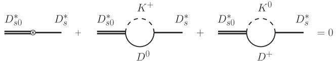
Figure 1: The mass renormalization mechanism that ensures that the $D_{s0}^{*}$ and $D_{s}^{*}$ do not mix for the physical particles. The loops are evaluated at $p^{2}=M_{D_{s0}^{*}}^{2}$. Double lines denote molecules, single lines charmed mesons, and dashed lines kaons.

Since the longitudinal components of the vector fields, $\partial_{\mu}P_{a}^{*\mu}$, have scalar quantum numbers, hadronic loops couple them to the scalar fields. In this way, the longitudinal components of the vector fields contribute to the self-energy of the scalar field. Analogously, the longitudinal components of the axial vectors couple to the pseudoscalar fields. Thus, for the purpose of renormalization, we have to add the counterterms

$$\mathscr{L}_{\text{long.}}=C_{DK}D_{s0}^{*}\left(\mathcal{D}_{\mu}D_{s}^{*\dagger\mu}\right)-C_{D^{*}K}\left[\left(\mathcal{D}_{\mu}D_{s1}^{*\mu}\right)D_{s}^{\dagger}-i\varepsilon_{\mu\nu\alpha\beta}v^{\alpha}D_{s1}^{\mu}D_{s}^{*\dagger\beta}\right]\ ,$$ (10)

with the coupling constants $C_{DK}$ and $C_{D^{*}K}$ adjusted to cancel the loops at the poles, cf. Fig. 1 and Ref. [24].

Furthermore, the Lagrangian for the leading contact interactions for the radiative decays reads

$$\mathscr{L}_{\rm Contact} \!\!= \!\!\kappa F_{\mu\nu}\left(v^{\mu}D_{s0}^{*}D_{s}^{*\dagger\nu}+D_{s1}^{\mu}v^{\nu}D_{s}^{\dagger}+\varepsilon^{\mu\nu\alpha\beta}{D_{s1}}_{\alpha}D^{*\dagger}_{s\beta}\right)$$ (11)

$$\!\!+\tilde{\kappa}\varepsilon^{\mu\nu\alpha\beta}F_{\mu\nu}v_{\beta}D_{s1,\alpha}D_{s0}^{*\dagger}+\text{h.c.}$$

We will discuss the relative importance of contact interactions and loop diagrams in a CHPT power counting scheme in Sec. 3.2.

For numerical calculations, we will take the following values for the meson masses [37]:

$$\begin{array}[]{lll}M_{D^{0}}=1864.86~{}\mathrm{MeV},&M_{D^{+}}=1869.62~{}\mathrm{MeV},&M_{D_{s}^{+}}=1968.49~{}\mathrm{MeV},\\ M_{D^{*0}}=2006.98~{}\mathrm{MeV},&M_{D^{*+}}=2010.28~{}\mathrm{MeV},&M_{D_{s}^{*+}}=2112.3~{}\mathrm{MeV},\\ M_{B^{+}}=5279.25~{}\mathrm{MeV},&M_{B^{0}}=5279.58~{}\mathrm{MeV},&M_{B^{0}}=5366.77~{}\mathrm{MeV},\\ M_{B^{*+}}=5325.2~{}\mathrm{MeV},&M_{B^{*0}}=5325.2~{}\mathrm{MeV},&M_{B_{s}^{*0}}=5415.4~{}\mathrm{MeV},\\ M_{\pi^{0}}=134.98~{}{\rm MeV},&M_{\pi^{+}}=139.570~{}\mathrm{MeV},&M_{\eta}=547.85~{}{\rm MeV},\\ M_{K^{+}}=493.677~{}\mathrm{MeV},&M_{K^{0}}=497.614~{}\mathrm{MeV}.&\end{array}$$

It is important to also specify the uncertainties of the mass differences used in our approach: $M_{D^{+}}-M_{D^{0}}=(4.8\pm 0.2)~{}\mathrm{MeV}$, $M_{D^{*+}}-M_{D^{*0}}=(3.3\pm 0.2)~{}\mathrm{MeV}$, $M_{B^{+}}-M_{B^{0}}=(-0.33\pm 0.24)~{}\mathrm{MeV}$, $M_{B^{*+}}-M_{B^{*0}}=(-0.33\pm 0.24)~{}\mathrm{MeV}$ [37]. The mass splittings in the charm and bottom sectors have different patterns because the interference between the $m_{d}-m_{u}$ contribution and the electromagnetic contribution is different [38].

3 Two-Body Decays

3.1 Hadronic Decays

In this section, we calculate the hadronic decay widths $D_{s0}^{*}\to D_{s}\pi^{0}$ and $D_{s1}\to D_{s}^{*}\pi^{0}$ and their corresponding bottom partners. The narrow widths of the charmed states can only be understood, if they are isoscalar states for then the pionic decays violate isospin. One natural decay mechanism, which is present irrespective of the assumed nature of the states, is the strong decay of the scalar (axial vector) state into a $D_{s}$ ($D_{s}^{*}$) and a virtual $\eta$-meson, followed by the isospin violating transition to a pion via the $\pi^{0}$-$\eta$ mixing amplitude $\epsilon_{\pi\eta}=0.013\pm 0.001$. This amplitude is analytic in the quark masses and scales as $(m_{u}-m_{d})/m_{s}$. Different groups using different underlying models for the $D_{sJ}$ states report hadronic widths due to the $\pi^{0}$-$\eta$ mixing ranging between 3 and 25 keV [5, 12, 14, 26, 22, 23].

For molecular states one more isospin violating mechanism exists, since they decay through meson loops [26, 22, 23]. Because the charged and neutral mesons have different masses, the meson loops of, for instance, $D^{+}K^{0}$ and $D^{0}K^{+}$ are different numerically. This difference introduces an additional, sizable isospin breaking that is specific for molecular states. In effect, most studies found hadronic widths for the hadronic molecules larger than $100$ keV. Especially, the most refined investigation including lattice data to fix higher-order operators finds a hadronic width of $(133\pm 22)$ keV [18].

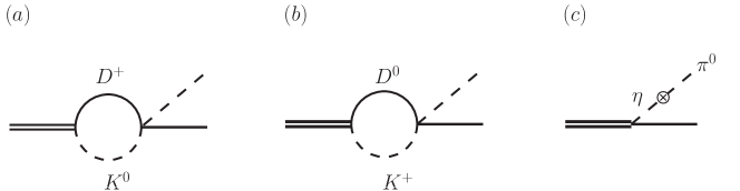
Figure 2: The two mechanisms that contribute to the hadronic width of the $D_{s0}^{*}$. (a) and (b) represent the nonvanishing difference for the loops with $D^{+}K^{0}$ and $D^{0}K^{+}$, respectively. (c) depicts the decay via $\pi^{0}$-$\eta$ mixing.

Table 2: Hadronic decay widths from different mechanisms.

Decays	loops	$\pi^{0}$-$\eta$ mixing	full result
$D_{s0}^{*}\to D_{s}\pi^{0}$	$(26\pm 3)~{}\mathrm{keV}$	$(23\pm 3)~{}\mathrm{keV}$	$(96\pm 19)~{}\mathrm{keV}$
$D_{s1}\to D_{s}^{*}\pi^{0}$	$(20\pm 3)~{}\mathrm{keV}$	$(19\pm 3)~{}\mathrm{keV}$	$(78\pm 14)~{}\mathrm{keV}$
$B_{s0}\to B_{s}\pi^{0}$	$(8\pm 5)~{}\mathrm{keV}$	$(6\pm 6)~{}\mathrm{keV}$	$(0.8\pm 0.8)~{}\mathrm{keV}$
$B_{s1}\to B_{s}^{*}\pi^{0}$	$(7\pm 4)~{}\mathrm{keV}$	$(5\pm 5)~{}\mathrm{keV}$	$(1.8\pm 1.8)~{}\mathrm{keV}$

In our formalism, the isospin violating decays are represented by the diagrams shown in Fig. 2. For the calculation of the loop diagrams, we put the heavy-light rescattering vertex on shell for two reasons. First, the off-shell effects contribute to subleading orders only. Second, we followed the same procedure when solving the scattering equations that led to the values of the residues in Eqs. (2) and (6). the results are given in Its first column lists the results from the meson loops, see Fig. 2 (a) and (b). Since the mass differences in the $D$ sector are significantly larger than in the see above, the contribution of the loops to the widths is significantly larger for the former than for the latter. The uncertainties are propagated from the uncertainties of the residues in Eqs. (2) and (6), as well as those of the LECs for the heavy-light rescattering vertex. When the widths are calculated exclusively from $\pi^{0}$-$\eta$-mixing, diagram (c) of Fig. 2, we find around $20~{}\mathrm{keV}$ in the charm sector and about $5~{}\mathrm{keV}$ in the bottom sector, see the second column of Table 2. The difference can be explained by the much larger phase space in the charm sector.

The last column of Table 2 lists the full result, showing that interference effects play an important role. The differences between the bottom and charm sectors are even larger for the full result since interference between the two mechanisms is vastly different. The uncertainties for the full results are obtained by adding the uncertainties for the individual contributions linearly. This is done to incorporate the fact that the residues, $g_{DK}$ and $g_{D_{s}\eta}$ in the case of $D_{s0}^{*}$, are not necessarily independent quantities while they contribute largely to the uncertainties in the individual channels, respectively.

Note that our results differ significantly from the phenomenological studies of Ref. [39]. There, the predicted hadronic widths for the $B^{(*)}K$ molecules are much larger, in the range from 50 to 90 keV. The reason is that therein the masses of the molecules predicted in Refs. [12, 14] were used, which are around 100 MeV larger than those calculated in this paper, see Table 1. We checked that, if we keep all the LECs to the best fit values of Ref. [18], and only change the subtraction constant to produce a mass of $B_{s0}^{*}$ at 5725 MeV used in Ref. [39], then we obtain a larger width of 73 keV, which is consistent with the result in Ref. [39].

3.2 Radiative Decays

3.2.1 Power Counting

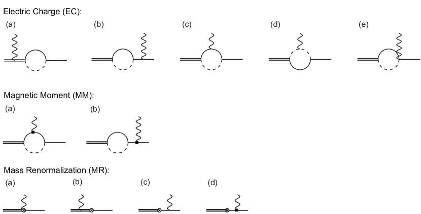
Figure 3: Different contributions to the radiative decays. In this case, the dashed lines denote kaons only. A photon coupling to the magnetic moment is denoted by a filled box.

We first address the relative size of the different contributions. We employ here the standard power counting scheme of CHPT coupled to heavy fields [40, 41, 42]. The relevant momentum scale is $p\sim\sqrt{2\mu\epsilon}\sim m_{K}$. The integration measure counts as $\mathcal{O}\left(p^{4}\right)$, the light meson propagator as $\mathcal{O}\left(p^{-2}\right)$ and the heavy one as $\mathcal{O}\left(p^{-1}\right)$. Similarly, the coupling of a photon to the electric charge gives $\mathcal{O}\left(p^{2}\right)$ for light and $\mathcal{O}\left(p\right)$ for heavy mesons. The field strength tensor of the photon, relevant for the coupling to the magnetic moments and the contact interaction, enters as $\mathcal{O}\left(p^{2}\right)$. The hard scale in CHPT is given by $\Lambda_{\chi}\sim 1~{}\mathrm{GeV}$. Thus, higher orders are suppressed by positive powers in $p/\Lambda_{\chi}$.

Consider first the one-loop diagrams where the photon couples to the electric charge of the involved mesons. For a photon emission inside the loop from a light meson, Fig. 3 EC(d), we find a factor of $\mathcal{O}\left(p^{-5}\right)$ from two light and one heavy propagators, plus the axial vector coupling as $\mathcal{O}\left(p\right)$, and the coupling of a photon to the electric charge of a light meson as $\mathcal{O}\left(p^{2}\right)$, so that this diagram counts in total as

$$\mathcal{O}\left(p^{4}\frac{1}{p^{5}}p^{3}\right)=\mathcal{O}\left(p^{2}\right).$$ (12)

Here, we have counted the $S$-wave coupling of the generated state to $D^{(*)}K$ as $\mathcal{O}\left(p^{0}\right)$. The same process with a charged intermediate heavy meson, Fig. 3 EC(c), gives

$$\mathcal{O}\left(p^{4}\frac{1}{p^{4}}p^{2}\right)=\mathcal{O}\left(p^{2}\right).$$ (13)

All other diagrams in the same set are of the same order, as required by gauge invariance. Since the contact interactions are proportional to the photon field strength tensor, they also contribute at order $p^{2}$. This means that there is no enhancement of the loop diagrams compared with the contact term and, contrary to the hadronic decays, we expect different models for the $D_{s}^{*}$ structure to lead to similar results. Below we will use the available data to fix the contact interaction in one channel in order to predict the others.

We also consider the contributions from the magnetic couplings of the heavy mesons. The size of the diagrams in Fig. 3 MM(a) are estimated as

$$\mathcal{O}\left(p^{4}\frac{1}{p^{4}}p^{3}\right)\sim\mathcal{O}\left(p^{3}\right).$$ (14)

They are thus suppressed by one order in $p/\Lambda_{\chi}$ relative to the LO. We will still calculate them for two reasons. First, the explicit calculation of a higher-order correction provides a measure of how well the chiral expansion converges. Secondly, all electric couplings vanish for the $D_{s1}\to D_{s0}^{*}\gamma$ and $B_{s1}\to B_{s0}\gamma$ transitions, so that the decays via the hadron loops contribute formally only at subleading order, while the leading contact term $\tilde{\kappa}$ in Eq. (11) enters for this channel at $\mathcal{O}\left(p^{2}\right)$. However, the corresponding loop is enhanced since it scales with the product of the residues for the coupling of the molecules to the continuum. We therefore conclude that no quantitative conclusions can be drawn for the $D_{s1}\to D_{s0}^{*}\gamma$ and $B_{s1}\to B_{s0}\gamma$ decays.

Typical further higher order diagrams include an additional pion exchange in the loop. This leads to additional factors of order $(p/\Lambda_{\chi})^{2}$, which imply that they can be safely neglected. The largest subleading contribution stems from the NLO term for the axial vector coupling. It is suppressed by one order, $p/\Lambda_{\chi}$, and we will use it to estimate the theoretical uncertainty for the amplitudes.

We close with some technical remarks. The diagrams in the first line of Fig. 3 show the full gauge invariant set of diagrams for which the photon couples to the electric charge. These are obtained by gauging the kinetic terms and the axial vector coupling. In Ref. [34] the explicit expressions for the amplitudes of all possible transitions are given. An explicit calculation confirms that the two subsets ($D^{0}K^{+}$ and $D^{+}K^{0}$ for $D_{s0}^{*}$) are gauge invariant separately, but there is still a remaining divergence. However, once the mass renormalization diagrams shown in the last line of Fig. 3 are included, all divergences are cancelled leaving a renormalized divergence-free amplitude.

In Ref. [26] vector and axial vector states are treated in the tensor formulation [43, 44]. In our approach, we modify the standard treatment of the vector formulation by employing a trick introduced by Stückelberg (see, for instance, Ref. [45]). The standard Lagrangian for an arbitrary vector particle $V$ with mass $m_{V}$ reads

$$\mathscr{L}_{V}=-\frac{1}{2}V^{\mu\nu}V_{\mu\nu}^{\dagger}+m_{V}^{2}V^{\mu}V_{\mu}^{\dagger}$$ (15)

with the field strength tensor $V_{\mu\nu}=D_{\mu}V_{\nu}-D_{\nu}V_{\mu}$ and the covariant derivative $D_{\mu}=\partial_{\mu}-i\,e\,A_{\mu}+\ldots$, where the ellipses indicate the presence of additional terms not relevant for the following discussion and $A_{\mu}$ denotes the photon field. The propagator resulting from this Lagrangian is

$$\frac{i}{l^{2}-m_{V}^{2}+i\varepsilon}\left(\frac{l^{\mu}l^{\nu}}{m_{V}^{2}}-g^{\mu\nu}\right),$$ (16)

with $l$ the vector meson momentum. This may make calculations rather extensive. Therefore, one may add another term to the Lagrangian that vanishes for on-shell vector particles:

$$\mathscr{L}_{V}=-\frac{1}{2}V^{\mu\nu}V_{\mu\nu}^{\dagger}+m_{V}^{2}V^{\mu}V_{\mu}^{\dagger}-\lambda(D_{\mu}V^{\mu})(D^{\nu}V_{\mu}^{\dagger})$$ (17)

and thus the propagator changes to

$$\frac{i}{[l^{2}-m_{V}^{2}+i\varepsilon]}\left(\frac{1-\lambda}{\lambda}\frac{l^{\mu}l^{\nu}}{[l^{2}-m_{V}^{2}/\lambda+i\varepsilon]}+g^{\mu\nu}\right).$$ (18)

where we are free to choose $\lambda=1$. Since we are dealing with radiative decays it is important to notice that also after gauging the coupling to a photon changes. For a much more detailed discussion of vector meson Lagrangians and the Stückelberg construction, we refer the reader to the comprehensive review [46].

3.2.2 Results

Table 3: The decay widths (in keV) calculated only from the coupling to the electric charge (EC), from the magnetic moments (MM) and from the contact term (CT), respectively, compared to the total (including interference). The CT strength for the transitions to odd parity mesons is fixed to data, while that to even parity states, marked as ’?’, is undetermined and part of the uncertainty.

Decay Channel	EC	MM	CT	Sum
$D_{s0}^{*}\rightarrow D_{s}^{*}\gamma$	$2.0$	$0.03$	$3.3$	$9.4$
$D_{s1}\to D_{s}\gamma$	$4.2$	$0.2$	$11.3$	$24.2$
$D_{s1}\to D^{*}_{s}\gamma$	$9.4$	$0.5$	$10.3$	$25.2$
$D_{s1}\to D_{s0}^{*}\gamma$	–	$1.3$	?	$1.3$
$B_{s0}\rightarrow B_{s}^{*}\gamma$	$22.4$	$0.6$	$5.2$	$32.6$
$B_{s1}\to B_{s}\gamma$	$39.4$	$25.8$	$5.1$	$4.1$
$B_{s1}\to B^{*}_{s}\gamma$	$46.5$	$0.1$	$6.4$	$46.9$
$B_{s1}\to B_{s0}\gamma$	–	$0.02$	?	$0.02$

Our amplitudes consist of three different contributions. For the decays via heavy meson-kaon loops, we considered the coupling of the photon to the electric charges and to the magnetic moment of the heavy mesons, as well as the contact interaction. In Table 3, we show the central values for the width calculated using one of the three contributions exclusively while discarding the remaining ones. With the contact interaction fixed to data as described below, the largest contribution comes from the loop diagrams where the photon couples to the electric charges. Coupling the photon to magnetic moments, which is of one order higher, gives in general small contributions. Therefore, the chiral expansion converges well. The magnetic contribution to the transition $D_{s1}\to D_{s0}^{*}\gamma$ is larger than the others in the charm sector, since it scales, as expected, with the product of two sizable resonance couplings $g_{DK}g_{D^{*}K}$, while all others scale with the product of one of them and the axial coupling constant $g_{\pi}$ for the $D^{*}D_{s}K$ vertex.

Two results stand out here and need to be explained. In the decay $B_{s1}\to B_{s}\gamma$ the contribution from the magnetic moment is particularly large because of a constructive interference that does not appear in any of the other channels. Individually, the interfering diagrams do not contribute more than expected from the power counting. However, this large contribution interferes destructively with the electric charge contribution. This leads, in turn, to a width about one order of magnitude smaller than those for the $B_{s1}\to B_{s}^{*}\gamma$ and $B_{s0}\to B_{s}^{*}\gamma$, despite of having the largest phase space. The same mechanism is not present in the other channels for different reasons. In the case of of the corresponding open charm decay, $D_{s1}\to D_{s}\gamma$, the charge of the heavy quark, $2/3$ instead of $-1/3$, prevents a similar effect. For the other open bottom channels $B_{s0}\to B_{s}^{*}\gamma$ and $B_{s1}\to B_{s}^{*}\gamma$ the relevant loops give too small contributions. The second interesting result is the small decay width for $B_{s1}\to B_{s0}\gamma$. Here we notice that the decay width scales with $E_{\gamma}^{3}/M_{B_{s1}}^{2}$. When we compare this to the same factor in the charm equivalent, we find a suppression of $\sim 1/150$, explaining the tiny decay width.

Table 4: Results for the relevant decay channels, compared to PDG 2012 [37]. The ^∗ denotes an input quantity.

	Our Result	Exp		Our Result	Exp
$R_{1}$	$0.10\pm 0.04$	$<0.059$	$R_{5}$	$0.98\pm 0.01$	$0.93\pm 0.09$
$R_{2}$	$0.38\pm 0.17^{\ast}$	$0.38\pm 0.05$	$R_{6}$	$0.37\pm 0.17$	$0.35\pm 0.04$
$R_{3}$	$0.40\pm 0.16$	$<0.16$	$R_{7}$	$0.39\pm 0.16$	$<0.24$
$R_{4}$	$0.02\pm 0.02$	$<0.22$	$R_{8}$	$0.02\pm 0.02$	$<0.25$

The currently available data are rather limited. Only upper limits exist for some decay widths, while others are not yet measured at all. The only available ratios are:

$$R_{1}:=\frac{\Gamma(D_{s0}^{*}\rightarrow D_{s}^{*}\gamma)}{\Gamma(D_{s0}^{*}\rightarrow D_{s}\pi^{0})},\qquad R_{2}:=\frac{\Gamma(D_{s1}\rightarrow D_{s}\gamma)}{\Gamma(D_{s1}\rightarrow D_{s}^{*}\pi^{0})},$$

$$R_{3}:=\frac{\Gamma(D_{s1}\rightarrow D^{*}_{s}\gamma)}{\Gamma(D_{s1}\rightarrow D_{s}^{*}\pi^{0})},\qquad R_{4}:=\frac{\Gamma(D_{s1}\rightarrow D_{s0}^{*}\gamma)}{\Gamma(D_{s1}\rightarrow D_{s}^{*}\pi^{0})},$$

$$R_{5}:=\frac{\Gamma(D_{s1}\rightarrow D_{s}^{*}\pi^{0})}{\Gamma(D_{s1}\rightarrow D_{s}^{*}\pi^{0})+\Gamma(D_{s1}\rightarrow D_{s0}^{*}\gamma)},$$

$$R_{6}:=\frac{\Gamma(D_{s1}\rightarrow D_{s}\gamma)}{\Gamma(D_{s1}\rightarrow D_{s}^{*}\pi^{0})+\Gamma(D_{s1}\rightarrow D_{s0}^{*}\gamma)},$$

$$R_{7}:=\frac{\Gamma(D_{s1}\rightarrow D^{*}_{s}\gamma)}{\Gamma(D_{s1}\rightarrow D_{s}^{*}\pi^{0})+\Gamma(D_{s1}\rightarrow D_{s0}^{*}\gamma)},$$

$$R_{8}:=\frac{\Gamma(D_{s1}\rightarrow D_{s0}^{*}\gamma)}{\Gamma(D_{s1}\rightarrow D_{s}^{*}\pi^{0})+\Gamma(D_{s1}\rightarrow D_{s0}^{*}\gamma)}.$$ (19)

In Table 4, we compare our results to the experimental values. We have chosen the ratio $R_{2}$ to fix the free parameter, namely the strength of the contact interaction $\kappa$ in Eq. (11). The same term contributes to the decays $D_{s0}^{*}\to D_{s}^{*}\gamma$, $D_{s1}\to D_{s}\gamma$ and $D_{s1}\to D_{s}^{*}\gamma$. However, an independent contact term $\tilde{\kappa}$ in Eq. (11) contributes to $D_{s1}\to D_{s0}^{*}\gamma$. We thus assign an uncertainty of 100% to this transition amplitude. The uncertainties include those from neglecting higher order contributions and of the coupling constants. Within the theoretical uncertainties, all results agree with the measured ratios or upper limits. The only possible exception is $R_{3}$, which is consistent only within two standard deviations. In our approach, almost identical values are found for each of the pairs of ratios $R_{2}$ and $R_{6}$, $R_{3}$ and $R_{7}$ since $\Gamma(D_{s1}\rightarrow D_{s}^{*}\pi^{0})\gg\Gamma(D_{s1}\rightarrow D_{s0}^{*}\gamma)$, in line with the observed proximity of $R_{2}$ and $R_{6}$.

Table 5: Results for the radiative decay widths in keV. The first column gives our result with all uncertainties from higher orders and coupling constants added in quadrature. The numbers in the second column are from a parity doubling model by Bardeen et al. [5]; in the third from light-cone sum rules by Colangelo et al. [47]; and in the fourth from Lutz and Soyeur [26], who provide two values with reasonable estimates for their remaining free parameter. The fifth column reports model calculations by Faessler et al. [22, 25, 39].

Decay Channel	Our Results	[5]	[47]	[26]	[22, 25, 39]
$D_{s0}^{*}\to D_{s}^{*}\gamma$	$(9.4\pm 3.8)$	$1.74$	$4-6$	$1.94(6.47)$	0.55-1.41
$D_{s1}\to D_{s}\gamma$	$(24.2\pm 10.7)$	$5.08$	$19-29$	$44.50(45.14)$	2.37-3.73
$D_{s1}\to D^{*}_{s}\gamma$	$(25.2\pm 9.7)$	$4.66$	$0.6-1.1$	$21.8(12.47)$	–
$D_{s1}\to D_{s0}^{*}\gamma$	$(1.3\pm 1.3)$	$2.74$	$0.5-0.8$	$0.13(0.59)$	–
$B_{s0}\to B_{s}^{*}\gamma$	$(32.6\pm 20.8)$	$58.3$	–	–	3.07-4.06
$B_{s1}\to B_{s}\gamma$	$(4.1\pm 10.9)$	$39.1$	–	–	2.01-2.67
$B_{s1}\to B_{s}^{*}\gamma$	$(46.9\pm 33.6)$	$56.9$	–	–	–
$B_{s1}\to B_{s0}\gamma$	$(0.02\pm 0.02)$	$0.0061$	–	–	–

Table 5 contains the results for the individual radiative decay widths. The theoretical uncertainties given there contain various contributions, we only show the sum of all added in quadrature. The largest uncertainty stems from the chiral expansion, which is estimated by multiplying the amplitudes by $(1\pm\sqrt{2\mu\epsilon}/\Lambda_{\chi})$, followed by the uncertainty of the contact term propagated from the error of the data used to fix it. Smaller uncertainties come from the residues and the axial vector coupling $g_{\pi}$, determined from the pionic decay of the $D^{*}$. In the case of the latter improved experimental data on the $D^{*}$ width would be helpful.

In absence of experimental information, we can compare our results only to the results of previous calculations which are given in the table as well, where the values in the last two columns were based on the hadronic molecular picture of the $D_{s0}^{*}$ and $D_{s1}$. Another result in the molecular picture was performed by Gamermann et al. [24], using an flavor-SU(4) Lagrangian, with a width of $0.475^{+0.831}_{-0.290}$ keV for the $D_{s0}^{*}\to D_{s}^{*}\gamma$.

The results by Lutz and Soyeur [26] are the closest to ours, while other calculations generally find smaller numbers. However, the differences are not large: all results, even those from the parity-doubling model for the $c\bar{s}$ mesons [5], agree with ours within two standard deviations. Similarly, the values from different models in the bottom sector agree within three standard deviations. This is however only based on our uncertainties. Once other models quote their residual error as well, the statistical significance of any deviation will decrease.

In contrast to this, the hadronic width is enhanced significantly for molecular states due to an additional loop contribution, but here the leading contact interaction is proportional to $(m_{u}-m_{d})E_{\pi}$ and thus suppressed. Consequently, calculations performed for compact $c\bar{s}$ states predict significantly smaller values. In contradistinction, the origins of larger contributions for molecular states are the two-particle cuts in meson loops, resulting in total widths of the order of $100~{}\mathrm{keV}$, and a larger coupling constant in Eq. (2). As can be seen in Eq. (1), the pure molecule sets an upper bound for $\lambda^{2}$, with an uncertainty of $\mathcal{O}\left(R\sqrt{2\mu\epsilon}\right)$. In principle, the $D^{(*)}K$ meson loops can also contribute to the width of the $c\bar{s}$ mesons. However, the coupling constant would be much smaller since $\lambda^{2}\ll 1$ for such states.

Similar to the charm sector, all values in the bottom sector from different models agree within three standard deviations, and less when the hitherto-unknown uncertainties of other models are considered.

4 Summary and Conclusion

We presented hadronic and radiative decay widths of the charm-strange resonances $D_{s0}^{*}(2317)$ and $D_{s1}(2460)$ under the assumption that they are $D^{(*)}K$ bound states. Our results are in fair agreement with available data. In detail, the decay widths are larger by more than one order of magnitude for the isospin violating hadronic decays than for the radiative decays: the hadronic widths are around 100 keV while the radiative ones are of the order of a few keV.

Our analysis revealed that only the hadronic decays are sensitive to a possible molecular component of both the $D_{s0}^{*}$ and $D_{s1}$— a hadronic width of 100 keV or larger can be regarded as a unique feature for molecular states. This experimental accuracy could possibly be reached with $\overline{\text{P}}$ANDA at the future accelerator facility FAIR. The origin of this enhanced width is the presence of two-meson cuts and the large coupling constant of the molecules to their constitutents—those should be much smaller in for non-molecular states. In contrast to this, the radiative decays turn out to be similar in size for all models for the states of interest. From the effective field theory point of view, this can be understood by the presence of a counterterm at LO, which is of short-distance nature, in these decays.

We also made predictions for their heavy flavor partners in the open bottom sector. Larger binding energies lead to much reduced hadronic widths. Since the radiative decay widths are much larger than those of the strong decays, radiative decays appear to be the most promising discovery channels for these positive parity bottom-strange mesons in future experiments.

References

- [1] S. Godfrey and N. Isgur, Phys. Rev. D 32, 189 (1985).
- [2] B. Aubert et al. [BaBar Collaboration], Phys. Rev. Lett. 90, 242001 (2003) [hep-ex/0304021].
- [3] D. Besson et al. [CLEO Collaboration], Phys. Rev. D 68, 032002 (2003) [Erratum-ibid. D 75, 119908 (2007)] [hep-ex/0305100].
- [4] M. A. Nowak, M. Rho and I. Zahed, Phys. Rev. D 48, 4370 (1993) [hep-ph/9209272].
- [5] W. A. Bardeen, E. J. Eichten and C. T. Hill, Phys. Rev. D 68, 054024 (2003) [hep-ph/0305049].
- [6] M. A. Nowak, M. Rho and I. Zahed, Acta Phys. Polon. B 35, 2377 (2004) [hep-ph/0307102].
- [7] F.-K. Guo, C. Hanhart and U.-G. Meißner, Phys. Rev. Lett. 102, 242004 (2009) [arXiv:0904.3338 [hep-ph]].
- [8] T. Barnes, F. E. Close and H. J. Lipkin, Phys. Rev. D 68, 054006 (2003) [hep-ph/0305025].
- [9] E. van Beveren and G. Rupp, Phys. Rev. Lett. 91, 012003 (2003) [hep-ph/0305035].
- [10] E. van Beveren and G. Rupp, Eur. Phys. J. C 32, 493 (2004) [hep-ph/0306051].
- [11] E. E. Kolomeitsev and M. F. M. Lutz, Phys. Lett. B 582, 39 (2004) [hep-ph/0307133].
- [12] F.-K. Guo, P.-N. Shen, H.-C. Chiang, R.-G. Ping and B.-S. Zou, Phys. Lett. B 641, 278 (2006) [hep-ph/0603072].
- [13] Y.-J. Zhang, H.-C. Chiang, P.-N. Shen and B.-S. Zou, Phys. Rev. D 74, 014013 (2006) [hep-ph/0604271].
- [14] F.-K. Guo, P.-N. Shen and H.-C. Chiang, Phys. Lett. B 647, 133 (2007) [hep-ph/0610008].
- [15] S. Weinberg, Phys. Rev. 130, 776 (1963).
- [16] D. Mohler, C. B. Lang, L. Leskovec, S. Prelovsek and R. M. Woloshyn, Phys. Rev. Lett. 111, 222001 (2013) [arXiv:1308.3175 [hep-lat]].
- [17] C. B. Lang, L. Leskovec, D. Mohler, S. Prelovsek and R. M. Woloshyn, arXiv:1403.8103 [hep-lat].
- [18] L. Liu, K. Orginos, F.-K. Guo, C. Hanhart and U.-G. Meißner, Phys. Rev. D 87, 014508 (2013) [arXiv:1208.4535 [hep-lat]].
- [19] F.-K. Guo, L. Liu, U.-G. Meißner and P. Wang, Phys. Rev. D 88, 074506 (2013) [arXiv:1308.2545 [hep-lat]].
- [20] F.-K. Guo, C. Hanhart and U.-G. Meißner, Eur. Phys. J. A 40, 171 (2009) [arXiv:0901.1597 [hep-ph]].
- [21] J. Hofmann and M. F. M. Lutz, Nucl. Phys. A 733, 142 (2004) [hep-ph/0308263].
- [22] A. Faessler, T. Gutsche, V. E. Lyubovitskij and Y. -L. Ma, Phys. Rev. D 76, 014005 (2007) [arXiv:0705.0254 [hep-ph]].
- [23] F.-K. Guo, C. Hanhart, S. Krewald and U.-G. Meißner, Phys. Lett. B 666, 251 (2008) [arXiv:0806.3374 [hep-ph]].
- [24] D. Gamermann, L. R. Dai and E. Oset, Phys. Rev. C 76, 055205 (2007) [arXiv:0709.2339 [hep-ph]].
- [25] A. Faessler, T. Gutsche, V. E. Lyubovitskij and Y. -L. Ma, Phys. Rev. D 76, 114008 (2007) [arXiv:0709.3946 [hep-ph]].
- [26] M. F. M. Lutz and M. Soyeur, Nucl. Phys. A 813, 14 (2008) [arXiv:0710.1545 [hep-ph]].
- [27] T. Mehen and R. P. Springer, Phys. Rev. D 72, 034006 (2005) [hep-ph/0503134].
- [28] H.-Y. Cheng and F.-S. Yu, arXiv:1404.3771 [hep-ph].
- [29] M. Cleven, F.-K. Guo, C. Hanhart and U.-G. Meißner, Eur. Phys. J. A 47, 19 (2011) [arXiv:1009.3804 [hep-ph]].
- [30] D. Gamermann, E. Oset, D. Strottman and M. J. Vicente Vacas, Phys. Rev. D 76, 074016 (2007) [hep-ph/0612179].
- [31] D. Gamermann and E. Oset, Eur. Phys. J. A 33, 119 (2007) [arXiv:0704.2314 [hep-ph]].
- [32] M. Mai, P. C. Bruns and U.-G. Meißner, Phys. Rev. D 86, 094033 (2012) [arXiv:1207.4923 [nucl-th]].
- [33] U.-G. Meißner, U. Raha and A. Rusetsky, Eur. Phys. J. C 41, 213 (2005) [Erratum-ibid. C 45, 545 (2006)] [nucl-th/0501073].
- [34] M. Cleven, PhD thesis, University of Bonn, 2013.
- [35] J. F. Amundson, C. G. Boyd, E. E. Jenkins, M. E. Luke, A. V. Manohar, J. L. Rosner, M. J. Savage and M. B. Wise, Phys. Lett. B 296, 415 (1992) [hep-ph/9209241].
- [36] J. Hu and T. Mehen, Phys. Rev. D 73, 054003 (2006) [hep-ph/0511321].
- [37] J. Beringer et al. [Particle Data Group Collaboration], Phys. Rev. D 86, 010001 (2012).
- [38] F.-K. Guo, C. Hanhart and U.-G. Meißner, JHEP 0809, 136 (2008) [arXiv:0809.2359 [hep-ph]].
- [39] A. Faessler, T. Gutsche, V. E. Lyubovitskij and Y. -L. Ma, Phys. Rev. D 77, 114013 (2008) [arXiv:0801.2232 [hep-ph]].
- [40] J. Gasser and H. Leutwyler, Annals Phys. 158, 142 (1984).
- [41] J. Gasser and H. Leutwyler, Nucl. Phys. B 250, 465 (1985).
- [42] J. Gasser, M. E. Sainio and A. Svarc, Nucl. Phys. B 307, 779 (1988).
- [43] G. Ecker, J. Gasser, H. Leutwyler, A. Pich and E. de Rafael, Phys. Lett. B 223, 425 (1989).
- [44] B. Borasoy and U.-G. Meißner, Int. J. Mod. Phys. A 11, 5183 (1996) [hep-ph/9511320].
- [45] C. Itzykson and J.-B. Zuber, Quantum Field Theory, McGraw-Hill, 1980.
- [46] U.-G. Meißner, Phys. Rept. 161, 213 (1988).
- [47] P. Colangelo, F. De Fazio and A. Ozpineci, Phys. Rev. D 72, 074004 (2005) [hep-ph/0505195].