Redshift evolution of the dynamical properties of massive galaxies from SDSS-III/BOSS

Abstract

We study the redshift evolution of the dynamical properties of $\sim 180,000$ massive galaxies from SDSS-III/BOSS combined with a local early-type galaxy sample from SDSS-II in the redshift range $0.1\leq z\leq 0.6$. The typical stellar mass of this sample is $M_{\star}$$\sim 2\times 10^{11}$$M_{\odot}$. We analyze the evolution of the galaxy parameters effective radius, stellar velocity dispersion, and the dynamical to stellar mass ratio with redshift. As the effective radii of BOSS galaxies at these redshifts are not well resolved in the SDSS imaging we calibrate the SDSS size measurements with HST/COSMOS photometry for a sub-sample of galaxies. We further apply a correction for progenitor bias to build a sample which consists of a coeval, passively evolving population. Systematic errors due to size correction and the calculation of dynamical mass, are assessed through Monte Carlo simulations. At fixed stellar or dynamical mass, we find moderate evolution in galaxy size and stellar velocity dispersion, in agreement with previous studies. We show that this results in a decrease of the dynamical to stellar mass ratio with redshift at $>2\sigma$ significance. By combining our sample with high-redshift literature data we find that this evolution of the dynamical to stellar mass ratio continues beyond $z\sim 0.7$ up to $z>2$ as $M_{\rm dyn}$/$M_{\star}$$\sim(1+z)^{-0.30\pm 0.12}$ further strengthening the evidence for an increase of $M_{\rm dyn}$/$M_{\star}$ with cosmic time. This result is in line with recent predictions from galaxy formation simulations based on minor merger driven mass growth, in which the dark matter fraction within the half-light radius increases with cosmic time.

1. Introduction

Early-type galaxies play an important role in observational studies of galaxy formation and evolution. Tight empirical correlations between the observed dynamical and stellar population properties of early-type galaxies have been derived that set useful constraints to their formation histories. These are correlations between size (effective radius, $R_{\rm e}$), surface brightness and stellar velocity dispersion ($\sigma_{\rm e}$), i.e., the fundamental plane (FP, Dressler et al. 1987; Djorgovski & Davis 1987; Bender et al. 1992, 1993), the stellar mass plane (Hyde & Bernardi, 2009b; Auger et al., 2010), the fundamental manifold of galaxies (Zaritsky et al., 2008), as well as correlations between galaxy color and stellar population age and metal abundance with galaxy mass (see review by Renzini, 2006).

Such scaling relations represent a powerful phenomenological tool to study the co-evolution of baryonic and dark matter in galaxies. The latter has been studied extensively for the local galaxy population. The tightness of the FP has been used to constrain stellar population variations or dark matter content in galaxies (Renzini & Ciotti, 1993) or to study non-homology (Ciotti et al., 1996). Gerhard et al. (2001) studied the dynamical properties and dark halo scaling relations of giant elliptical galaxies, and found that the tilt of the FP is best explained by a stellar population effect and not by an increasing dark matter fraction with luminosity.

Cappellari et al. (2006), using data from the SAURON survey (de Zeeuw et al., 2002), suggested that dynamical to stellar mass-to-light ratios larger than one are due to dark matter, assuming a constant stellar initial mass function (IMF) (Kroupa, 2001) and using self-consistent models (see Cappellari et al., 2013a, for a review). Other studies based on Sloan Digital Sky Survey (SDSS, York et al. 2000) data came to the conclusions that there is an excess over the predictions of stellar population models with a fixed IMF which are luminosity dependent (Padmanabhan et al., 2004; Hyde & Bernardi, 2009a, b).

These conclusions have recently been revised in Cappellari et al. (2013b) by means of a large number of axysimmetric dynamical models including different representations of dark matter halos reporting a variation of IMF slope with galaxy mass. In fact, as highlighted by Thomas et al. (2011), for instance, dark matter fraction and IMF are highly degenerate. They studied a sample of Coma galaxies and their detailed decomposition into luminous and dark matter reveals that for low-mass galaxies there is a good agreement between dynamical masses with dark matter halo and lensing results (galaxies with a $\sigma\sim 200$ $\mathrm{km\;s}^{-1}$ are consistent with a Kroupa IMF). For higher-mass galaxies ($\sigma>200$ $\mathrm{km\;s}^{-1}$), the disagreement can be due to either a non constant IMF (Kroupa IMF under-predicts luminous dynamical masses for galaxies at $\sigma\sim 300$ $\mathrm{km\;s}^{-1}$) or to a dark matter component which follows the light (see also Wegner et al. 2012).

A promising complementary approach to detailed studies of local galaxies for breaking the degeneracy between dark matter fraction and IMF is to study the evolution of fundamental plane, dynamical and stellar population properties of galaxies with look-back time (Bender et al., 1998; van Dokkum et al., 1998; Treu et al., 2005; Jørgensen et al., 2006; Saglia et al., 2010; Houghton et al., 2012; Bezanson et al., 2013b). Moreover, dark matter fractions can also be studied in samples of lensed galaxies at different redshifts (see Bolton et al. 2012a using data from both the Sloan Lens ACS sample, SLACS, Bolton et al. 2006, Bolton et al. 2008, and the BOSS Emission line Lens Survey, BELLS, Brownstein et al. 2012).

A large number of such investigations have been performed in recent years, analyzing the redshift evolution of galaxy sizes (e.g., Daddi et al., 2005; Trujillo et al., 2006a, b, 2007; Longhetti et al., 2007; Zirm et al., 2007; Toft et al., 2007; van Dokkum et al., 2008; Buitrago et al., 2008; Cimatti et al., 2008; Franx et al., 2008; Bernardi, 2009; Damjanov et al., 2009; Saracco et al., 2009; Bezanson et al., 2009; Mancini et al., 2009, 2010; Valentinuzzi et al., 2010a; Carrasco et al., 2010; Szomoru et al., 2012; Newman et al., 2012; Saracco et al., 2014) and dynamical properties of galaxies (van der Wel et al., 2005, 2008; Cenarro & Trujillo, 2009; Cappellari et al., 2009; van Dokkum et al., 2009; Newman et al., 2010; Onodera et al., 2010; Saglia et al., 2010; van de Sande et al., 2011; Toft et al., 2012; Onodera et al., 2012; van de Sande et al., 2013; Damjanov et al., 2013; Belli et al., 2014). The bottom line is that galaxy sizes appear to decrease (at fixed stellar mass) and stellar velocity dispersions increase (at fixed stellar mass) with increasing look-back time. Some of these conclusions are still controversial, however. Tiret et al. (2011), for example, argue that the size evolution disappears when one homogenizes literature data sets by measuring the stellar mass with the same method and provides accurate estimates of the sizes to prevent systematic effects in the $R_{\rm e}$ measurements of low $S/N$ high-z compact galaxies (Mancini et al., 2009). Mancini et al. (2010) also report evidence for galaxies as large as local ones at redshift higher than 1.4 suggesting that not all high-$z$ galaxies are compact. Moreover, the effect depends on the photometric band and on whether galaxies have young or old light-weighted ages and if they reside in clusters or field (see Valentinuzzi et al. 2010b for clusters and Poggianti et al. 2013 for field studies; see also Trujillo et al. 2011 for a different opinion).

So far, galaxies in the distant Universe (look-back times of a few billion years and above) have not been studied at the same statistical level as local galaxies. The new data set from the Baryon Oscillation Spectroscopic Survey (BOSS, Dawson et al. 2013) as part of the Sloan Digital Sky Survey-III (SDSSIII, Eisenstein et al., 2011) provides the opportunity to investigate the dynamical and stellar population properties of a galaxy sample of unprecedented size up to redshifts $z\sim 0.7$. The survey is currently obtaining spectroscopic data for nearly 1.5 million massive galaxies at redshifts between 0.2 and 0.7, hence up to look-back times of $\sim 6\;$Gyr. The combination of this sample with local early-type galaxies from SDSS-I/II allows us to make a statistically significant link between local galaxy properties and higher redshift observations. This is the main aim of the present paper.

The paper is organized as follows. The galaxy sample is described in Section 2. Photometric, kinematic, and dynamical properties are presented in Section 3, as well as the calibration technique for measuring the effective radii based on a sub-sample of galaxies with HST photometry and the correction for progenitor bias. The results are presented in Section 4 and discussed in Section 5. The paper concludes with Section 6.

Throughout the paper we assume the following cosmology with $H_{0}=71.9$ $\mathrm{km\;s^{-1}\;Mpc^{-1}}$, $\Omega_{\rm m}=0.258$, and $\Omega_{\Lambda}=0.742$ following the cosmology used for the stellar mass determination of BOSS galaxies in DR9 (Maraston et al., 2013).

2. Data

We use the galaxy sample from SDSS-III/BOSS covering a redshift range $0.2\lesssim z\lesssim 0.7$. To leverage our study on the redshift evolution we combine this sample with a local sample of massive galaxies at $z\sim 0.1$ drawn from SDSS-II.

2.1. Main galaxy sample from SDSS-III/BOSS

Data are taken from the SDSS-III/BOSS Data Release Nine (DR9, Ahn et al. 2012). BOSS (Dawson et al., 2013; Smee et al., 2013), one of the four surveys of SDSS-III (Eisenstein et al., 2011), is taking spectra for 1.5 million luminous massive galaxies with the aim of measuring the cosmic distance scale and the expansion rate of the Universe using the Baryonic Acoustic Oscillations (BAO) scale (Anderson et al., 2012). Data are taken with an upgraded version of the multi-object spectrograph on the SDSS telescope (Gunn et al., 2006). BOSS galaxy targets are selected from the SDSS ugriz imaging (Fukugita et al., 1996; Gunn et al., 1998; Stoughton et al., 2002), including new imaging part of DR8 mapping the southern Galactic hemisphere. A series of color cuts have been used to select targets for BOSS spectroscopy (Padmanabhan et al. 2014, in preparation). The selection criteria are designed to identify a sample of luminous and massive galaxies with an approximately uniform distribution of stellar masses following the Luminous Red Galaxy (LRG, Eisenstein et al. 2001) models of Maraston et al. (2009). The galaxy sample is composed of two populations: the higher redshift Constant Mass Sample (CMASS, $0.4<z<0.7$) and the Low-Redshift Sample (LOWZ, $0.2<z<0.4$). A fraction (around 1/3) of those LOWZ galaxies derived with those cuts have been already observed in SDSS-I/II and are included in the BOSS sample, but they are not re-observed if they had reliable redshifts. These two population are well separated in the $(g-r)$ and $(r-i)$ colors diagram (Masters et al., 2011).

To extract a working set of objects from the entire BOSS sample we matched galaxies from different catalogs of stellar velocity dispersions and stellar masses described in the following Sections using the keywords PLATE, MJD, FIBERID that uniquely determine a single observation of a single object. The final merged catalog comprises $491,954$ galaxies that are included in DR9. We selected objects from the LOWZ and CMASS samples (BOSS_TARGET1 = Target flags) with a good platequality (PLATEQUALITY=’good’), with object class ’galaxy’ (class_noqso=GALAXY), with high-confidence redshifts (ZWARNING_NQSO=0), and for which we have a unique set of objects in the case of duplicate observations (SPECPRIMARY=1).

The final sample we will analyze comprises $\sim 180,000$ objects (37% of the original sample) obtained after applying some additional redshift cuts and quality cuts to stellar velocity dispersions and stellar masses that we will discuss in Section 3.

2.2. Local galaxy sample from SDSS-II

In order to connect our BOSS galaxies to the local galaxy population, we use a sample of galaxies from the SDSS Data Release Seventh (DR7, Abazajian et al., 2009). We select early-types galaxies following Hyde & Bernardi (2009a). Galaxies had to be well fitted by a de Vaucouleurs profile in the $g$ and $r$-bands (fracDeV_g=1 fracDeV_r=1), with an early-type like spectrum (eClass $<$ 0), extinction-corrected $r$-band de Vaucouleurs magnitudes in the range $14.5<$deVMag_r$<17.5$ (this results in a tighter limit compared to that of the SDSS Main Galaxy sample, see details in Hyde & Bernardi 2009a), measured stellar velocity dispersion in DR7 velDisp $>0$, and with an axis ratio in $r$-band of $b/a>0.6$, to be more likely pressure supported. As described in Hyde & Bernardi (2009a) the DR7 $b/a$ distribution shows two distinct populations separated by this axis-ratio value with a 20% of low-luminosity objects at $b/a<0.6$. This retains $\sim 123,500$ DR7 objects.

Bernardi et al. (2010) did a detailed comparison of different methods to select early-types in the literature (morphologically based, colors, or structural parameters-based methods), showing that Hyde & Bernardi (2009a) cuts give similar results to other methods but is more efficient in discriminating elliptical galaxies from spirals, which is important in our analysis.

We select galaxies with zWarning$=0$ and apply some constraints on the errors of the parameters: errors on $R_{\rm e}<$70%, errors on the axis ratios $0<err_{b/a}<1$, errors in $\sigma<$30%. Only galaxies with stellar velocity dispersion of 70$<$$\sigma$$<$550$\mathrm{km\;s}^{-1}$ were selected, following the BOSS cuts.

3. Galaxy properties

The primary aim of this work is to study the redshift evolution of the dynamical properties of BOSS galaxies. Stellar masses are taken from Maraston et al. (2013) and stellar velocity dispersions from Thomas et al. (2013). Both of these quantities are included in the DR9 data release. We used a sub-sample of 240 galaxies with additional HST/COSMOS photometry and BOSS spectra (Masters et al., 2011) to derive a calibration for galaxy sizes from DR8. In the following sections we describe the galaxy parameters in more detail. In Section 3.4 we describe how the effective radii and stellar velocity dispersion are combined to derive virial masses.

The redshifts used in our analysis are those extracted from DR9 as z_noqso with formal $1\sigma$ error given by z_err_noqso (outputs of the BOSS pipeline as described in Bolton et al. 2012b and Schlegel et al. 2014, in preparation). Redshifts are successfully determined for $\sim 98\%$ of CMASS galaxies (Anderson et al., 2012, their Table 1). Errors in the measured redshift are less than about 0.0002 ($\sim 60$ $\mathrm{km\;s}^{-1}$). BOSS observed a few galaxies at $z>0.7$ and $z<0.2$. In our analysis we focus on the redshift range $0.2\leq z\leq 0.7$ and therefore excluded all the galaxies outside this redshift range. This cut retains 90% of the galaxies ($444,118$ objects).

3.1. Stellar mass

We use the stellar masses $M_{\star}$ from Maraston et al. (2013) as published in the DR9 data release. These masses are derived through broad-band spectral energy distribution (SED) fitting of model stellar populations on SDSS $u,g,r,i,z$ modelMag magnitudes from DR8, scaled to the $i$-band cmodelMag magnitude. The BOSS spectroscopic redshift is used to constrain the fits. We note that the DR9 data release also provides alternative mass estimates from Chen et al. (2012) (see Maraston et al., 2013, for discussion).

Maraston et al. (2013) use different types of templates to derive stellar masses; passive models, star-forming models or a mix, chosen so as to match the galaxy expected galaxy type, based on a color cut, in BOSS. In this paper we used stellar masses obtained with the passive template that is a mix of old populations with a spread in metallicity and which was found to reproduce well the colors of luminous red galaxies at redshift 0.4 to 0.7 (Maraston et al., 2009). This maximally old and passive LRG template minimizes the risk of underestimating $M_{\star}$ which is the typical effect that occurs when one determines stellar masses from light (Maraston et al., 2010; Pforr et al., 2012).

We adopt the stellar masses derived from the median of the probability distribution function (PDF). Typical uncertainties on $M_{\star}$ are $<0.1\;$dex, independently of redshift (see Maraston et al., 2013, for details).

The Portsmouth stellar mass pipeline described in Maraston et al. (2013) provides stellar masses using various types of configurations, i.e. Kroupa (2001) or Salpeter (1955) IMF, passive (Maraston et al., 2009) or star-forming (Maraston et al., 2006) models, and considering or not the mass-loss in the stellar evolution. The subset of calculations used here adopt a Kroupa IMF. As is well known, a Salpeter IMF produces systematically larger stellar masses by about a factor 1.6 (Maraston, 2005; Bolzonella et al., 2010). Systematic uncertainties are mainly due to the choice of the IMF ($\sim 0.2\;$dex).

We removed galaxies for which $M_{\star}$ was not properly determined due to unreliable values of redshift and photometry issues. This cut retains 387,590 galaxies (79% of the full sample).

3.2. Size

The photometric data used in this paper were derived using the SDSS-III DR8 pipeline (Aihara et al., 2011). One of the main updates performed in DR8 compared to Stoughton et al. (2002) is the correction for sky levels (in particular for extended galaxies) which past studies found to be overestimated (Bernardi et al., 2007; Lauer et al., 2007; Guo et al., 2009). This issue has also been addressed in detail in Blanton et al. (2011). SDSS effective radii are adopted from the DR8 catalog. In this section we describe this measurement and its calibration with COSMOS/HST imaging.

3.2.1 SDSS DR8 effective radii

Effective radii are estimated using seeing-corrected de Vaucouleurs effective radii (deVRad) and the associated errors (deVRadErr, of the order of $\sim 5-25$ % depending on redshift). Those values correspond to the effective radius along the semi-major axis derived on elliptical aperture.

BOSS galaxies are often not well resolved in SDSS imaging. The average seeing of the SDSS survey is 1$\farcs$05 from the PSF_FWHM in the $i$-band (lower and upper percentile of 0$\farcs$88 to 1$\farcs$24), which is better than in previous data releases due to the repeated images taken during the survey (see Ross et al., 2011; Masters et al., 2011). The median effective radius of BOSS galaxies (after having applied the previous cuts on the sample) is 1$\farcs$24 (upper and lower percentile 2$\farcs$12 and 0$\farcs$72, respectively). As a consequence, seeing effects will affect size measurements (see Saglia et al. 1993, Saglia et al. 1997, Bernardi et al. 2003), which we need to correct for. To develop a seeing correction we compare SDSS galaxy radii with measurements based on high-resolution HST/COSMOS imaging (Section 3.2.3).

The surface brightness models used by pipeline to obtain galaxy sizes are relatively simple (single parameter fits, i.e. exponential or de Vaucouleurs profiles); a more complex model is not feasible for this analysis because of the limitation of the image resolution. We tested this conclusion and found that performing Sérsic fits on BOSS images yields strong degeneracies between effective radius and Sérsic index, preventing robust estimate of effective radii. We estimate SDSS circularized radii as $R_{\rm e,circ}=R_{\rm e}\times q^{1/2}$ where $R_{\rm e}$ is the semi-major axis of the half-light ellipse and $q=b/a$ is the axis ratio which is part of the DR8 catalog.

The effective radii should, in principle, be referred to a fixed rest-frame wavelength to account for the fact that early-types have color gradients, so on average their optical radii are larger in bluer bands and at higher $z$ this effect will make the sizes larger (see Bernardi et al., 2003; Hyde & Bernardi, 2009a, for discussions). We did not apply any correction for this trend, because uncertainties of the size calibration ($\sim$ 10-25%) are larger than the typical variation in size measured in different filters (from 4% to 10%, Bernardi et al. 2003, Hyde & Bernardi 2009a). In Section 4.1 we describe the average effect this could have on the size evolution studies.

Effective radii were converted to physical radii using the code of Hogg (1999) which presents the scale conversion between arcsec and kpc for our given cosmology. Hereafter, we will use the notation pipeline $R_{\rm e}$ to represent SDSS effective radii in kpc. We further remove from the catalogs galaxies with unreliable values of $R_{\rm e}$ and their errors. This cut retains $\sim 370,000$ objects.

3.2.2 COSMOS effective radii

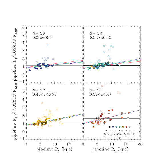
Figure 1.— Ratio between pipeline $R_{\rm e}$ from SDSS DR8 and COSMOS $R_{\rm e,Ser}$ as a function of pipeline $R_{\rm e}$. Points are coded as a function of redshift ($0.2\leq z\leq 0.3$, $0.3<z\leq 0.45$, $0.45<z<0.55$, and $0.55\leq z\leq 0.7$). Different lines represent different fitting procedures: the red line is a linear fit, the green line is a linear fit with one $2\sigma$ clip, the blue line is iterative $2\sigma$ clipping, the horizontal black line is the single offset. Circles are the points that have been used in the fit and open squares are points discarded in the iterative sigma clipping. Open stars are multiple systems in HST imaging which are unresolved in the SDSS images (Masters et al., 2011). Labels in each panel give the number of galaxies used in the fit including objects discarded in the iterative $2\sigma$ clipping (multiple systems are not included in this number).

Masters et al. (2011) constructed a sub-sample of 240 BOSS galaxies with HST/COSMOS imaging (Koekemoer et al., 2007; Leauthaud et al., 2007). This sample was used to calibrate the SDSS DR8 radii part of the CMASS sample. We adopted the effective radii from the public Zurich Structure & Morphology Catalog v1.0 (Scarlata et al., 2007; Sargent et al., 2007) derived from $I$-band (F814W) ACS images. Effective radii are available from this catalog for 224 of the 240 objects.

The catalog contains galaxy structural parameters derived from a two-dimensional decomposition using the GIM2D code (Galaxy Image 2D, Simard, 1998) on the ACS/HST images as deep as $I_{\rm AB}\sim 22.5$ (Sargent et al., 2007). We used the seeing-corrected effective radii R_GIM2D resulted from the one component Sérsic fit, of the form

$$I(r)=I_{\rm e}10^{[-b_{n}((r/R_{\rm e,"})^{1/n}-1)]}$$ (1)

where $I_{\rm e}$ is the effective intensity, and the constant $b_{n}$ is defined in terms of the shape parameter n and is chosen so that $R_{\rm e,"}$ encloses half of the total luminosity and it is measured in arcsec. The quantity $b_{n}$ can be well approximated by $b_{n}=0.868n-0.142$ (Caon et al., 1993). The Zurich Structure & Morphology Catalog v1.0 contains two values of the effective radius from GIM2D, R_GIM2D and R_0P5_GIM2D which correspond to the PSF-corrected effective radii. The choice of one of the two is purely arbitrary and they show a negligible median difference of 0$\farcs$001 (with R_GIM2D being smaller than R_0P5_GIM2D). The catalog gives the uncertainties on effective radii as 99% confidence lower and upper error on R_GIM2D (LE_R_GIM2D, UE_R_GIM2D, respectively). Those errors are $<1$% of R_GIM2D, much smaller than the errors in $R_{\rm e}$ from SDSS photometry ($\sim 15$ % in the COSMOS/BOSS sub-sample).

Sizes are converted to circularized effective radii $R_{\rm e,serc}$ following the procedure described in Saglia et al. (2010) which calculates the half-light radius obtained from the classical curve of growth analysis of the intrinsic Sérsic profile. The procedure requires R_GIM2D, Sérsic index SERSIC_N_GIM2D, and axis ratio $q=b/a$, where $a$, $b$ are the semi-major and minor axis of the half-light ellipse, and $q=1-\epsilon$, where $\epsilon$ is the ellipticity of the object ELL_GIM2D. Here we use a different parametrization than in Section 3.2.1 because we have additional information from the Sérsic fit (the two parametrization would give consistent results for a wide range of $q$).

We did not apply any correction to account for the fact that rest-frame wavelengths are different at different redshifts using only $i$-band data because this sample is only used for calibration purposes, and uncertainties due to the size calibration we derive using COSMOS radii are much larger than the wavelength variation at the redshifts considered (see Section 3.2.1). Moreover COSMOS has just one filter available for those galaxies. COSMOS radii were converted to kpc in the same way as SDSS radii using the code of Hogg (1999). Hereafter, we will use the notation COSMOS $R_{\rm e,Ser}$ to represent COSMOS effective radii in kpc.

3.2.3 Comparison SDSS vs COSMOS

A significant fraction (23 %) of BOSS galaxies with HST imaging are unresolved multiple systems in SDSS imaging (Masters et al., 2011). To derive an accurate calibration we excluded these unresolved multiple systems from our analysis (44 galaxies) using the public catalog of Masters et al. (2011) . The redshift range we wish to study is $0.2\leq z\leq 0.7$, and we discarded 4 additional galaxies at higher redshifts and 13 at $z<0.2$. This leaves us a sample of 163 galaxies. COSMOS redshifts are adopted, as not all of these objects (158 out of 163) have BOSS redshifts (this will not change our results, because the median difference between COSMOS and BOSS redshifts is negligible, 7.21$\times 10^{-6}$). We do not correct for PSF variations in the SDSS imaging, because the PSF is reasonably stable and the effect is negligible compared to the overall correction derived here.

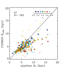
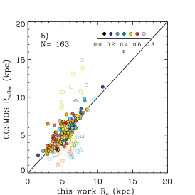
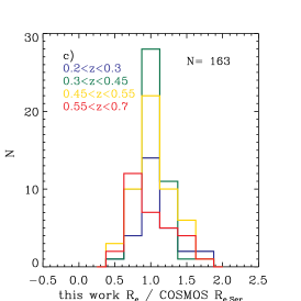
Figure 2.— Left panel: COSMOS $R_{\rm e,Ser}$ as a function of pipeline SDSS $R_{\rm e}$ coded in terms of redshift. Central panel: COSMOS $R_{\rm e,Ser}$ as a function of rescaled SDSS $R_{\rm e}$ (used in the present work) coded in terms of redshift. Symbols are as in Figure 1. Right panel: Distribution of the ratio between SDSS rescaled $R_{\rm e}$ and COSMOS $R_{\rm e,Ser}$ for the four redshift bins in Figure 1. Histograms contain also discarded objects but not multiple systems. Legends in each panel give the number of galaxies used in the derivation of the size correction including objects discarded in the iterative $2\sigma$ clipping (multiple systems are not included in this number).

Figure 1 shows the ratio between SDSS and COSMOS effective radii as a function of SDSS effective radius for four redshift bins. The ratio is around $1.1$ and SDSS radii can be overestimated by up to a factor two. The discrepancy between SDSS and COSMOS radii increases with increasing SDSS radius (see also Masters et al., 2011). Masters et al. (2011) found that a single offset was reproducing their data in which they compared the ratio SDSS over COSMOS radii as a function of COSMOS radii. In this work we compare the ratio of SDSS over COSMOS radii as a function of SDSS radii to derive a correction for the full BOSS sample. As is to be expected, there is also some redshift dependence, in the sense that SDSS radii overestimate most the true radii at higher redshifts. Also, as expected, the scatter of the relationships increases with redshift owing to the decrease in SDSS imaging quality.

The size calibration could be affected by the larger uncertainties in the SDSS effective radii due to the higher than typical sky background ($\geq$ 60-70%) of SDSS images in the COSMOS field (Masters et al., 2011; Mandelbaum et al., 2012) (on the other side seeing is smaller than typical of 10-15%) which could give relations between SDSS and COSMOS radii not universal for the full BOSS sample.

We performed fits to these relationships in the four redshift bins independently. We tested for linear correlations applying different levels of sigma clipping in the linear fits: no sigma clipping, red line in Figure 1; just one $2\sigma$ clipping green line in Figure 1; and an iterative $2\sigma$ clipping blue line in Figure 1 with a maximum of three iterations.

We fitted a linear relation of the form $R_{\rm e,pipeline}/R_{\rm e,COSMOS,Ser}=a+b(R_{\rm e,pipeline})$. The best-fit quantities $a$ and $b$, the number of galaxies used in the fit after the sigma clipping, the scatter of the relations $c$ (which include objects discarded by the $2\sigma$-clipping) and their associated errors obtained as $1\sigma$ uncertainties for each redshift bin are listed in Table LABEL:tab:sizecorr. The least-square fits were performed using the MPFIT algorithm (Markwardt, 2009) under the IDL environment. Fits with and without sigma clipping are consistent within the errors.

The slope of the relation increases slightly with redshift as to be expected. The scatter about the relation is comparable in the first three redshift bins, while the last redshift bin shows a considerably higher scatter (see Table LABEL:tab:sizecorr, $c=0.49\pm 0.06$). For this reason, we will only use the first three redshift bins in the analysis.

We tested the significance of the fits through an F-test by comparing the resulting $\chi^{2}$ values for free and fixed slope fits accounting for the number of degrees of freedom, and find a maximum probability of no relation to be $\sim$2 %, which confirms the statistical validity of our fits. The final fits we adopt for the radius correction in each redshift bin are the linear fits with iterative $2\sigma$ clipping (blue lines) because they give corrections with a smaller scatter compared to other fits (of 6-30%). The open squares in Figure 1 are those galaxies that were discarded in the sigma clipping. Open stars represent unresolved multiple systems not considered in the fits.

We additionally searched for correlations of the effective radius with several other DR8 structural parameters like axis ratio b/a, fracdev, and the difference between fiber2mag and modelmag with the aim at finding the best parameter space for the radius correction. None of these parameters helped improving the radius correction.

The size correction we derive here accounts also for the fact that galaxies in our sample could have been better described by a Sérsic profile rather than a de Vaucouleurs, therefore we should consider our calibrated sizes as ”Sérsic-like”.

Table 1Size correction for the four redshift bins.

$z$ range	$N$	$a$	$b$	$c$
$0.2\leq z\leq 0.3$	24	0.84 $\pm$0.11	0.04 $\pm$0.01	0.29$\pm$ 0.04
$0.3<z\leq 0.45$	48	0.75 $\pm$0.06	0.06 $\pm$0.01	0.19$\pm$ 0.02
$0.45<z<0.55$	41	0.75 $\pm$0.04	0.07 $\pm$0.01	0.32$\pm$ 0.03
$0.55\leq z\leq 0.7$	30	0.97 $\pm$0.17	0.08 $\pm$0.02	0.49$\pm$ 0.06

Notes. — A correlation of the form $R_{\rm e,pipeline}/R_{\rm e,COSMOS,Ser}=a+b(R_{\rm e,pipeline})$ is assumed. $N$ is the number of points used in the fit after iterative $2\sigma$ clipping. Uncertainties on each parameter are 1$\sigma$ errors. The rms scatter $c$ is derived as deviation of the data about the fits considering also objects discarded by the $2\sigma$-clipping.

3.2.4 Radius calibration

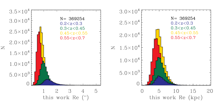
Figure 3.— Histogram of the effective radii derived in this work (after size correction), in arcseconds (left panel) and kpc (right panel) for various redshift bins as color-coded in Figure 2.

Figure 2 middle panel b) shows the final corrected radii that are obtained using the fits of Figure 1. For comparison the left a) panel shows the uncorrected radii. Panel c) presents the distribution of the ratio between the SDSS and COSMOS radii in various redshift bins after the correction. The radii agree well at all redshifts after the correction has been applied. More specifically, the median ratio between our rescaled $R_{\rm e}$ and COSMOS $R_{\rm e,Ser}$ is 1.02 (upper and lower quartile 1.34, 0.86 and mean 1.10) for $0.2\leq z\leq 0.3$, 0.98 (upper and lower quartile 1.15 and 0.85 and mean 1.01) for $0.3<z\leq 0.45$, 1.01 (upper and lower quartile 1.31 and 0.84 and mean 1.05) for $0.45<z<0.55$, and 0.99 (upper and lower quartile 1.41 and 0.73 and mean 1.02) for $0.55\leq z\leq 0.7$. Median values of the distributions in each redshift are compatible within $\pm 1\sigma/N^{1/2}$, where $N$ is the number of objects. Typical errors on rescaled radii range from 0.7 kpc at $z\sim 0.2$ to 1.0 kpc at $z\sim 0.7$ and median radii range from 5.34 to 4.28 kpc, mode 4.73 to 3.48 kpc, in this redshift range. If we did not apply the size correction we would have larger radii (median sizes range from 5.72 kpc at $z\sim 0.25$ to 5.40 kpc at $z\sim 0.55$, 6.51 kpc at $z\sim 0.65$, mode from 5.00 to 4.00 kpc and 5.00 at $z\sim 0.65$).

Filled circles in Figure 2 are those galaxies that were used in the previous section to derive the calibration. Open squares are those objects that were discarded in the iterative $2\sigma$ clipping. Open stars are the unresolved multiple systems discarded from the calibration. Most of the multiples are strong outliers in these plots and they would have been discarded during the sigma clipping fit.

Figure 3 shows the resulting distributions of galaxy effective radii (in both arcseconds and kpc) for the final sample of 369,254 galaxies in the various redshift bins. The size distribution can be described by a log-normal function (as the typical size distribution at low redshift, Shen et al. 2003; Bernardi et al. 2003) but with different peaks of the distributions suggesting a variation of typical sizes with $z$. In Section 4 we present our results using both the corrected SDSS size and pipeline sizes (which we circularized using SDSS axis ratio for this purpose).

3.2.5 Systematic errors

The systematics in the error budget have been assessed through Monte Carlo simulations which account for uncertainties in both parameters $a$ and $b$ of the fit. The average errors vary with redshift in a non-linear fashion. The errors are $\sim 0.6$ kpc at $z\sim 0.25$, $\sim 0.2$ kpc at $z\sim 0.55$, and $\sim 0.6$ kpc at $z\sim 0.65$.

We additionally include in our Monte Carlo simulations the impact of unresolved multiple systems, which have systematically overestimated sizes. By using the COSMOS/BOSS sub-sample we can estimate that those correspond to the $\sim$ 6% of the galaxies in this sample (see left panel of Figure 13). The sizes of the two components which are resolved in the COSMOS imaging (and unresolved in the SDSS imaging) allow us to assess the contribution of unresolved multiple systems in our analysis, which seems to be negligible compared to other systematic uncertainties (see Appendix B for details).

More detail on the Monte Carlo simulations are given also in Section 4, where we discuss the impact on the final science analysis.

3.3. Stellar velocity dispersion

Stellar velocity dispersions ($\sigma$) are taken from the Portsmouth Spectroscopic pipeline described in Thomas et al. (2013), also available in DR9. Briefly, stellar kinematics are derived by means of the Penalized Pixel-Fitting method pPXF (Cappellari & Emsellem, 2004) in spectra in which emission lines are fitted with Gaussian templates by using the GANDALF code (Sarzi et al., 2006). The stellar population models of Maraston & Strömbäck (2011) have been adopted to fit the stellar continuum. These are based on a hybrid model between MILES stellar library (Sánchez-Blázquez et al., 2006) and theoretical spectra at bluer wavelengths from UVBLUE (Rodríguez-Merino et al., 2005). Stellar population models based on the MILES library have a resolution of 2.54 Å FWHM (Beifiori et al., 2011), and therefore needed to be only slightly downgraded to match the BOSS spectral resolution ($R\sim 1800-2000$ at $5000\;$Å, 2.78 Å $-$2.50 Å FWHM). Stellar velocity dispersions have been measured in the typical rest-frame wavelength range $4500-6500$ Å most suitable for stellar kinematics analysis due to the presence of strong absorption features (Bender, 1990; Bender et al., 1994).

Stellar velocity dispersions from the Portsmouth Spectroscopic pipeline agree within a few percent with other DR9 measurements of $\sigma$ by Bolton et al. (2012b) and Chen et al. (2012) (see Thomas et al., 2013, for a detailed comparison of the systematic offsets between methods). Thomas et al. (2013) show that the typical error distribution on the $\sigma$ measurements for BOSS galaxies peaks at 14 %, and 93 % of the measurements have an error below 30 %. We therefore selected objects with an error in $\sigma$ below 30 % for the present study to be as inclusive as possible while still maintaining an acceptable accuracy in velocity dispersion (large errors are due to the low signal-to-noise, S/N, of BOSS spectra, mean $\sim 4.4$ from S_N median, which is sufficient to measure velocity dispersions, Thomas et al. 2013). This cut is not as tight as is generally applied but it allows us not to be affected by biases due to sample selection (for example, a common tighter cut with a relative error $<$ 10% would discard most of the low $\sigma$ galaxies at high redshift). Thomas et al. (2013) also show that $\sigma$ determinations show no bias with $S/N$. Errors on $\sigma_{\rm e}$ slightly vary with redshift, from 12 $\mathrm{km\;s}^{-1}$ at $z\sim 0.25$ to 39 $\mathrm{km\;s}^{-1}$ at $z\sim 0.65$.

Besides the cut in relative error below 30% we further restrict our sample to values of $70\leq\sigma\leq 550$ $\mathrm{km\;s}^{-1}$. We discard velocity dispersions below 70 $\mathrm{km\;s}^{-1}$ because of the limit in instrumental resolution of the BOSS spectrograph, and velocity dispersions above 550 $\mathrm{km\;s}^{-1}$ to exclude contamination by potential multiple systems (Bernardi et al., 2003, 2006, 2008). The final number of galaxies that survive these additional cuts in velocity dispersion is $\sim 370,000$, which is 75 % of the original sample.

The stellar velocity dispersions from BOSS spectroscopy ($\sigma_{\rm ap}$) are measurements within the 2$\ \!\!{}^{\prime\prime}$ diameter aperture of the BOSS fiber. Therefore, we applied an aperture correction to translate the BOSS velocity dispersions to the aperture corresponding to the effective radius using the relation of Cappellari et al. (2006) derived from the integral field data of the SAURON sample

$$\sigma_{\rm e}=\sigma_{\rm ap}\times(r_{\rm ap}/R_{\rm e,"})^{0.066}$$ (2)

in which $\sigma_{\rm e}$ is the stellar velocity dispersion within $R_{\rm e,"}$, and $r_{\rm ap}=1$$\ \!\!{}^{\prime\prime}$ is the radius of the BOSS fiber. $R_{\rm e,"}$ is taken from the rescaled effective radii converted to arcsecond. The relation of Cappellari et al. (2006) is consistent with that of Mehlert et al. (2003, slope=0.06) and slightly steeper but in agreement within the errors with older determinations by Jorgensen et al. (1995, slope=0.04).

Aperture corrections depend on galaxy profile and systematic evolution in the light profile of galaxies could affect the stellar velocity dispersion, as well as this rescaling factor could change from local SAURON galaxies to the higher redshift BOSS galaxies. However, we expect this effect to be negligible as the aperture corrections are small (maximum 3% at higher redshift) because the fiber diameter is close to the typical effective radius of galaxies at the redshifts studied here (see Figure 3). Typical uncertainties after the aperture correction range from 5 to 16% of $\sigma_{\rm e}$ (13 to 39 $\mathrm{km\;s}^{-1}$).

3.3.1 Systematic errors

We performed Monte Carlo simulations to estimate systematic errors on the aperture correction due to the size calibration (see Section 3.2.4), and have found them to be small. On average $\sigma_{\rm e}$ changes by $\sim 1.5$$\mathrm{km\;s}^{-1}$, which is well below the measurements errors.

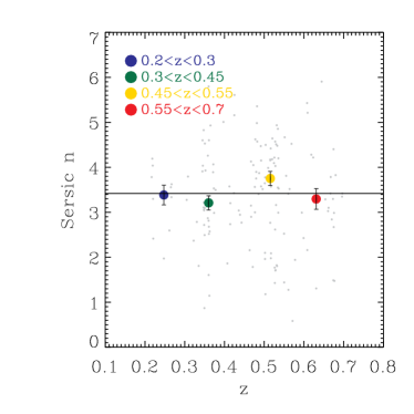
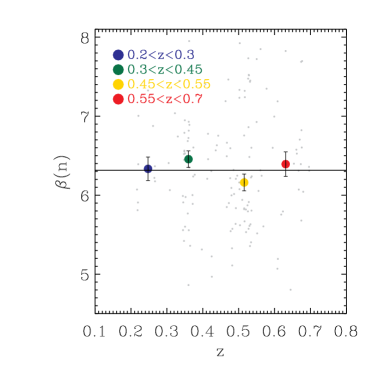
Figure 4.— Sérsic indices (left panel) and $\beta$ parameters (right panel, see Equation 3) of the COSMOS/HST sample for various redshift bins as color-coded in Figure 2. Colored symbols with error bars are the medians. The continuous line is the median value. The total number of objects is 150.

3.4. Dynamical mass

Following Beifiori et al. (2012), we estimate dynamical galaxy mass from the effective radius and velocity dispersion within the effective radius using the virial mass estimator as

$$M_{\rm dyn}=\beta(n)\;R_{\rm e}\sigma_{\rm e}^{2}/G$$ (3)

where $G$ is the gravitational constant and $\beta$ is a dimensionless constant that depends on galaxy structure, often adopted as $\beta=5.0\pm 0.1$ for local galaxies, see Cappellari et al. (2006).

Even though based on measurements within the effective radius, this virial estimator is designed to capture the total dynamical mass of a galaxy. A caveat is that this might only be true as long as total mass traces light. Thomas et al. (2011) found that this assumption might not be consistent with lensing studies. They suggest that Equation 3 may only yield about 86 % of the true total dynamical mass. However, this will only affect the absolute scale of the dynamical to stellar mass ratios that we derive, while their evolution with redshift will remain the same. As we are mostly interested in the latter, the main conclusions of this work will not be affected. As an additional check we therefore compared the $M_{\rm dyn}$/$M_{\star}$ derived here with those measured for local galaxies from more sophisticated dynamical modeling in and find good agreement (see Section 4.3). Still, it should be emphasized that any change in dynamical mass found here reflects a change of dynamical mass within $1R_{\rm e}$.

3.4.1 Dependence on structural parameters

The appropriate value of $\beta$ is actually a function of the Sérsic shape index n (Trujillo et al., 2004; Cappellari et al., 2006). Taylor et al. (2010) showed that dynamical masses and stellar masses correlate well when the structure of the galaxy is taken into account (see also Section 3.4.5). They find that dynamical masses estimated with the homology assumption exhibit residual trends with galaxy structure properties, so they introduce a structure-corrected dynamical mass adopting a constant $\beta$ that is Sérsic index dependent (Bertin et al., 2002). Note that the virial mass estimator of Cappellari et al. (2006) (Equation 3) has been calibrated on dynamical masses from Schwarzschild modeling where no assumption about homology is made.

For our sample of BOSS galaxies we cannot make any statements in this respect since SDSS images do not have the necessary angular resolution to perform Sérsic fits. However, we can expect this effect to be negligible, as the BOSS galaxy sample is restricted to massive galaxies in a relatively narrow mass range (Maraston et al., 2013) and limited redshift range so that variations of the Sérsic index will be minimal. Moreover, the fact that our size calibration is based on Sérsic $R_{\rm e}$ from COSMOS, allows us to account for possible differences between de Vaucouleurs profiles and Sérsic profiles resulting in a “Sérsic-like” calibrated radii.

We verify this assumption with the COSMOS sub-sample for which Sérsic indices are available. The Zurich Structure & Morphology Catalog v1.0 also contains values of galaxy Sérsic index, $n$. This allows us, for this sub-sample, to account for the variation of the parameter $\beta$ with $n$ and encapsulate the effects of galaxy structure on $M_{\rm dyn}$ (by assuming a constant $\beta$ for all galaxies Equation 3 implicitly assumes that all galaxies are homologous).

We estimate $\beta(n)$ following the analytic expression between $\beta(n)$ and the Sérsic index (Equation 20 of Cappellari et al., 2006), which is theoretically derived for spherical and isotropic models with a Sérsic profile for different values of $n$ (Bertin et al. 2002, see also Taylor et al. 2010 for a discussion of its importance on the SDSS sample).

Figure 4, right panel, shows the dependence of the $\beta(n)$ parameter on redshift for each galaxy in the sub-sample (gray points). Colored circles are the median $\beta(n)$ for each redshift bin. We find that the median $\beta(n)$ is $\sim 6.3$ for all redshifts bins (see continuous line in Figure 4, right panel). This is larger than the local values of 5 generally adopted, and yields systematically higher masses by $\sim$20%. The reason is the relatively low Sérsic indices (between 3.38 and 3.30 at $z\sim 0.25$ or $z\sim 0.6$, as shown in Figure 4, left panel) for the COSMOS sample, compared to typical Sérsic indices for local galaxies.

The key point illustrated by Figure 4, however, is that both $n$ and $\beta(n)$ do not evolve with redshift. As we focus in the redshift evolution and not absolute values for dynamical mass, the present study is not affected by a systematic offset in $\beta$. We will use $M_{\rm dyn}$ derived using a median $\beta=6.3$, which is the median value $\beta$ derived using the BOSS/COSMOS photometry.

3.4.2 Dependence on aperture

The dynamical mass obtained using the virial mass estimator (see Section 3.4) is based on stellar kinematics within an aperture of 1 effective radius and scaled to total dynamical mass via equation 3. This quantity is compared with the total stellar mass from Maraston et al. (2013) based on cmodelMag magnitudes. Hence both dynamical and stellar masses are total masses, which ensures a consistent comparison.

Still, the total dynamical mass is derived from observations within the effective radius, while the stellar mass comes from the total stellar light. We explore therefore the possible presence of a systematic effect from the different apertures in which kinematics and stellar populations have been measured. To this end we compare $M_{\star}$ derived from modelmag (rescaled to $i$-band cmodelmag) and $M_{\star}$ from aperture magnitudes within $R_{\rm e}$ (rescaled to $i$-band cmodelmag). This test is presented in Appendix A.

In brief, the difference between the two sets of masses is $\sim 0.08$ dex. The stellar masses measured from SED fitting within 1 $R_{\rm e}$ are higher by this amount, because of the higher $M/L$ ratio within $1R_{\rm e}$. We emphasize, however, that this quantity is an overestimate of the true total mass. Nevertheless, it is reassuring to verify that this systematic difference is relatively small. Most importantly, the offset is independent of redshift (see Appendix A). Hence the science analysis of this work is not affected, because we study redshift dependence and do not focus on absolute ratios between dynamical and stellar masses. We also note that the dynamical to stellar mass ratio is always larger than 0.08 dex in our redshift range, hence $M_{\star}$ does never exceed $M_{\rm dyn}$ ensuring physically meaningful solutions throughout.

3.4.3 Dependence on rotation

The possible presence of unresolved rotation is another complication that could affect our mass estimates from Equation 3. van der Marel & van Dokkum (2007) have measured increased rotational support at $z\sim 0.5$ and argue that data at different redshifts can be affected by rotation, with a stronger impact on low-$\sigma$ galaxies which are more rotationally supported than galaxies at high $\sigma$. As our BOSS sample consists of massive galaxies in a relatively small mass range (Maraston et al., 2013), however, we expect this effect to be negligible.

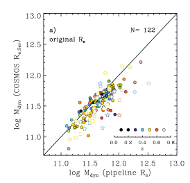
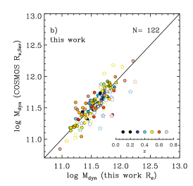
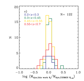
Figure 5.— Left panel: Dynamical masses derived using the original SDSS $R_{\rm e}$ assuming a constant $\beta=6.3$ versus dynamical masses derived using COSMOS $R_{\rm e,Ser}$ adopting a variable $\beta$ based on the Sérsic index. Symbols are as in Figure 1. Central panel: Same as left panel but using rescaled SDSS $R_{\rm e}$ adopted in the present study. Right panel: Distribution of the ratio of dynamical masses from rescaled SDSS $R_{\rm e}$ and COSMOS $R_{\rm e,Ser}$ for the four redshift bins of Figure 1. Legends in each panel give the number of galaxies used in the derivation of the size correction including objects discarded in the iterative $2\sigma$ clipping (multiple systems are not included in this number).

3.4.4 Dependence on galaxy type

Finally, in deriving $M_{\rm dyn}$ with Equation 3, we implicitly assume that the measured value of $\sigma_{\rm e}$ is dominated by the bulge component. For late-type galaxies we expect that the disc contribution to $\sigma_{\rm e}$ results in a broader distribution of $M_{\rm dyn}$, since the $\sigma_{\rm e}$ may not represent the actual dynamical state of those galaxies which is dominated by rotation (see Section 3.4.3) as well as the $\beta$ parameter we used could not be appropriate for late-type galaxies with low Sérsic index. As shown in Masters et al. (2011), however, the majority of BOSS galaxies ($74\pm 6$%) have early-type morphology and the remaining later types are bulge dominated, hence this effect will be negligible. We tested this assumption by only considering early-type galaxies for the CMASS sample using the morphological cut $(g-i)>2.35$ by Masters et al. (2011). We compared dynamical masses derived with COSMOS $R_{\rm e}$ and adopting $\beta$ based on the Sérsic index and dynamical masses with $R_{\rm e}$ derived in this work and found a good agreement between early-types and the full COSMOS/BOSS sub-samples, with a scatter around the one-to-one relation consistent within the errors ($\sim$0.14 dex).

3.4.5 Calibrated virial masses for the COSMOS sub-sample

As an additional test we compare our virial mass estimates based on the re-scaled effective radii with virial masses derived directly from the COSMOS effective radii, the result is shown in Figure 5. The left-hand panel shows the comparison between virial masses derived using COSMOS $R_{\rm e}$ and the uncorrected SDSS $R_{\rm e}$. As expected, there is a clear offset to higher virial masses from SDSS imaging because of the overestimation of galaxy radii.

The re-scaled radius of this work remedies this problem. The central panel of Figure 5 shows the comparison between virial masses derived using COSMOS $R_{\rm e}$, and adopting a variable $\beta$ based on the Sérsic index (see Section 3.4.1) and the corrected SDSS $R_{\rm e}$ of the present work (by using a constant $\beta=6.3$ as described in Section 3.4.1). Mass estimates agree well at all redshifts with a scatter of $\sim 0.14$ dex, which is well within the errors. The right-hand panel presents the distribution of the logarithmic ratio between COSMOS and SDSS masses after correction. The distribution is symmetric around zero for all redshift bins with a maximum deviation of $\sim$0.5 dex.

3.4.6 Random and systematic errors

The final errors in $M_{\rm dyn}$ are a combination of uncertainties in $\sigma_{\rm e}$ (which account for the aperture scaling of $\sigma$), $R_{\rm e}$, the statistical uncertainties due to the rescaling factor of $R_{\rm e}$, and $\beta$. This results in median random errors of $\sim 0.15$ dex depending on redshift (from 0.08 dex at $z=0.25$ to 0.18 dex at $z=0.65$). Based on Monte Carlo simulations we estimate median systematic errors due to the size calibration (see Section 3.2.4) and uncertainty of $\beta(n)$ to be $\sim$ 0.04 dex.

3.5. Local SDSS-II early-type galaxy sample

We combine the SDSS-III/BOSS sample described above with a local sample of massive galaxies at $z\sim 0.1$ drawn from SDSS-II. The galaxy properties of this local sample are presented in the following sections.

3.5.1 Stellar mass

Stellar masses and ages were estimated from the SED fitting of the $u,g,r,i,z$-band photometry following the same prescription of Maraston et al. (2013) with passive templates (the LRG model by Maraston et al. 2009 mentioned earlier). We homogenize the stellar mass distribution by selecting a sub-sample that matches the mass distribution of the BOSS sample. We constructed this sub-sample using the stellar mass distribution in the lowest BOSS redshift bin ($0.2<z<0.3$) as reference. For each stellar mass bin we randomly selected from the local galaxy distribution a number of galaxies equal to the number of galaxies in the low-$z$ BOSS one. This cut on the local early-types population retains $12,089$ galaxies. A discussion on the impact of the science analysis in this paper from this homogenization is given in Appendix E.

3.5.2 Size

We collect photometry and effective radii $R_{\rm e}$ from DR8 in which the correction for the sky over-subtraction of previous releases is already implemented (see discussion in Section 3.2.1) and no further correction to sizes (see Hyde & Bernardi 2009a for details) has been applied. This is motivated by the fact that we selected galaxies at redshift $z<0.2$ that are resolved in the SDSS imaging with $R_{\rm e}$$>$ FWHM of the PSF (retaining 96% of the objects).

3.5.3 Stellar velocity dispersion

We collect redshift and stellar velocity dispersions from the DR7 catalogs. Thomas et al. (2013) show that their DR7 $\sigma$ are consistent with SDSS pipeline $\sigma$ at the few percent level (see their Figure 1). The median offset across all the stellar velocity dispersion is $\sim$ 1%. However, this offset increases towards high stellar velocity dispersions. We can quantify the correct offset to apply to DR7 $\sigma$ looking at Figure 4 of Thomas et al. (2013) where their $\sigma$ are compared to Bolton et al. (2012a) $\sigma$ within BOSS, which is the relevant mass range.. The offset is 4%, which we correct for in the SDSS-II sample.

We further rescaled stellar velocity dispersions to the value at $R_{\rm e}$, following the procedure described in Section 3.3, accounting for the fact that DR7 galaxies were observed with a 3$\ \!\!{}^{\prime\prime}$ aperture. The variation in $\sigma_{\rm e}$ for the aperture correction in local SDSS galaxies is  2% ($\sigma_{\rm e}$ within Re on average 2% smaller than the SDSS ones, and median ratio between aperture size and $R_{\rm e}$ is $\sim$0.72).

3.5.4 Dynamical mass

Dynamical mass is derived from stellar velocity dispersion and size in the same way as for the BOSS sample as described in Section 3.4. To ensure internal consistency we use the same redshift independent parameter $\beta=6.3$ as for the BOSS sample derived from the BOSS/COSMOS photometry (see Section 3.4.1).

3.6. Correction for progenitor bias

BOSS target selection was designed to obtain a nearly uniform stellar mass distribution across the redshift range $0.2\leq z\leq 0.7$. Still, the sample needs to be corrected for effects from progenitor biases (e.g., Valentinuzzi et al., 2010b; Saglia et al., 2010; Cimatti et al., 2012, and references therein), as higher-$z$ galaxies in the sample are not necessarily progenitors of the lower-$z$ galaxies in the sample (see also Tojeiro et al., 2012).

To correct for the progenitor bias we compare – in each redshift bin – the galaxy ages from Maraston et al. (2013) (one of the products of the SED fit, see Section 3.1) and remove those galaxies from the low-$z$ sample whose ages (evolved to the highest redshift bin by subtracting the look-back time) would be lower than a given age threshold which is the time needed for a typical galaxy to become passive. For each redshift bin we select galaxies such that their age follows

$$t_{\rm g}(z)-(t_{\rm u}(z)-t_{\rm u}(z=0.65))>3Gyr$$ (4)

where $t_{\rm g}$ is the age of a galaxy at a give redshift, $t_{\rm u}$ is the age of the universe at the same redshift and $t_{\rm u}(z=0.65)$ is the age of the universe at the median redshift of the highest redshift bin. Histograms of the evolved ages for different redshift bins are shown in Figure 6. Galaxies in the shaded region have been discarded. As the age threshold we chose 3 Gyr, adopting the age limit used in Maraston et al. (2013) for calculating stellar masses (see their Section 3.1 for discussion). This threshold is only slightly larger than the 1.5 Gyr suggested by van Dokkum & Franx (2001).

We considered the highest redshift bin as a reference and we evolved all other redshift bins including the local SDSS early-type sample. By discarding galaxies with age$\;<3\;$Gyr, we retain 268,938 galaxies, which corresponds to the $\sim 65\%$ of the initial local and BOSS samples as shown in Figure 6.

We obtain similar results using the tighter selection criteria described in Cimatti et al. (2012), which select in each redshift bin the galaxies with ages within $\pm 1\sigma$ of the age distribution for each redshift bin accounting for the cosmic time elapsed from one bin to the other. This selection also discards objects at older ages and provides a sample size that is $\sim$54% of the initial one.

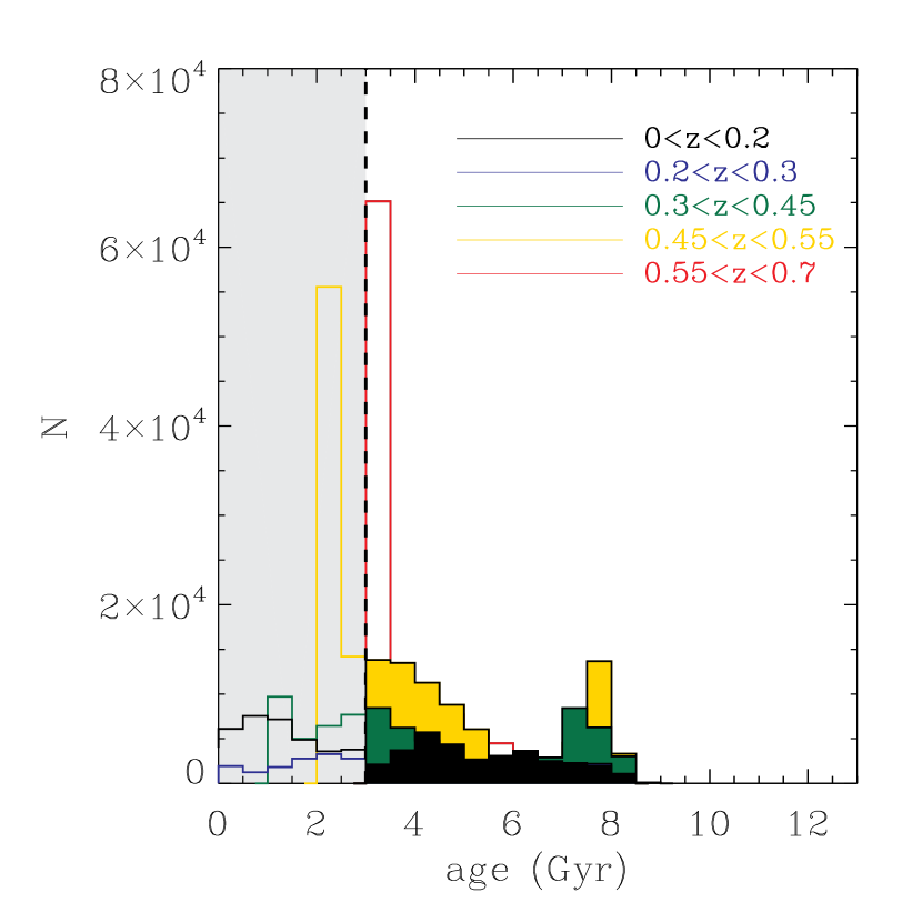
Figure 6.— Histograms of the ages for different redshift bins, evolved to the highest redshift bin by subtracting the look-back time, which are used to apply the progenitor-bias cut (see text for details). Galaxies in the shaded region, i.e., with an age below $3\;$Gyr, have been discarded.

Poggianti et al. (2013) found that galaxy sizes are correlated to luminosity-weighted ages such that older galaxies will show a stronger size evolution, with a stronger effect in clusters than in the field. Our progenitor bias correction minimizes that effect.

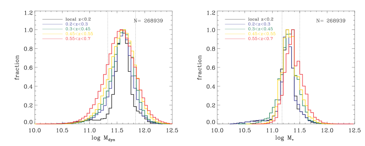
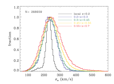
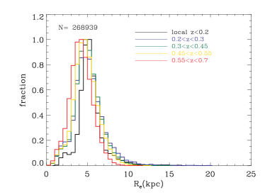
Figure 7.— Top panels: Distribution of $M_{\rm dyn}$ (with $\beta=6.3$, left panel) and $M_{\star}$ (right panel) for various redshift bins, normalized to the peak value in each bin. The BOSS mass distributions are fairly uniform over the redshift range under analysis (see also Figure 10 in Maraston et al. 2013). Local early-types from SDSS-II are selected to have the same stellar mass distribution of the lowest BOSS redshift bin. Dotted-black lines indicate the $\pm 1\sigma$ of the mass distributions adopted for the present analysis. Bottom left and right panels: distributions in stellar velocity dispersion distribution and effective radius. The progenitor-bias correction has been applied in all cases.

The distributions of $M_{\star}$, $M_{\rm dyn}$, $\sigma_{\rm e}$, and $R_{\rm e}$ of the final sample after correction for progenitor bias are shown in Figure 7 for various redshift bins. The typical median stellar mass is around $\log$$M_{\star}$$\sim 11.28$ dex, the median $R_{\rm e}$$\sim 5.2$ kpc, and $\sigma_{\rm e}\sim 231$ $\mathrm{km\;s}^{-1}$.

To study the effect of the progenitor bias correction on the redshift evolution of these quantities, we have performed a re-analysis for a sample without progenitor bias correction presented in Appendix D. It can be seen that generally results are consistent. Most importantly, the evolution of $M_{\rm dyn}$/$M_{\star}$ is fairly stable against the progenitor-bias correction, hence the main conclusions of these paper do not critically depend on the progenitor bias correction.

Table 2Fitting parameters for the redshift evolution of galaxy parameters between $0.1\leq z\leq 0.55$.

	$M_{\star}$		$M_{\rm dyn}$
Parameter	slope	zero point	slope	zero point
$R_{\rm e}$	$-0.49\pm 0.26$	$0.76\pm 0.04$	$-0.37\pm 0.20$	$0.73\pm 0.03$
$\sigma_{\rm e}$	$0.12\pm 0.02$	$2.36\pm 0.01$	$0.18\pm 0.06$	$2.35\pm 0.01$
$M_{\rm dyn}/M_{\star}$	$-0.48\pm 0.23$	$0.35\pm 0.03$	$-0.55\pm 0.17$	$0.36\pm 0.02$

Notes. — Uncertainties on each parameter are $1\sigma$ errors derived from Monte Carlo simulations. The relation we fitted for $R_{\rm e}$ is $\log R_{\rm e}=\log R_{\rm e,0}+\beta(1+z)$, for $\sigma_{\rm e}$ is $\log\sigma_{\rm e}=\log\sigma_{\rm e,0}+\gamma(1+z)$, and for $M_{\rm dyn}/M_{\star}$ is $\log(M_{\rm dyn}/M_{\star})=\log(M_{\rm dyn}/M_{\star})_{0}+\delta(1+z)$.

4. Results

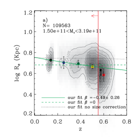
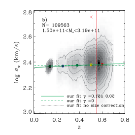
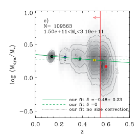
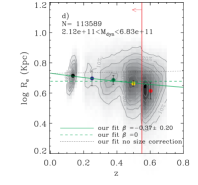
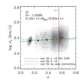
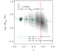
Figure 8.— Left panels: Effective radius $R_{\rm e}$ as a function of redshift. Central panels: Stellar velocity dispersion $\sigma_{\rm e}$ as a function of redshift. Right panels: Ratio between dynamical and stellar mass $M_{\rm dyn}$/$M_{\star}$ as a function of redshift. Top and bottom panels are for galaxies selected using $M_{\star}$ and $M_{\rm dyn}$, respectively (within $\pm 1\sigma$ of the mass distributions, total number of galaxies given by the labels). The shaded contour region indicates the full sample after correction for progenitor bias. Contours show 10 equally-spaced density levels showing the percentage of galaxies compared to the peak value of each plot. The colored filled circles are the median values in four redshift bins. The green solid line is a linear fit, the green dashed line is a fit with zero slope for comparison. The black dotted line is a linear fit to the sample if no size correction is applied. Error bars of the median points indicate the $1\sigma$ uncertainty derived from Monte Carlo simulations. The red-continuous lines and arrows indicate the range where we fit our data.

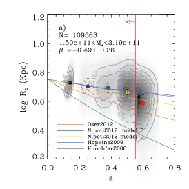
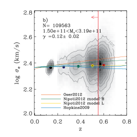
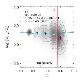
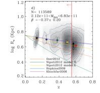
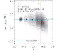
Figure 9.— Same as Figure 8 with predictions from theoretical models over-plotted as solid colored lines for comparison (see labels for references).

In this section we present the redshift evolution of the galaxy parameters effective radius, velocity dispersion, and dynamical to stellar mass ratio for our final sample of 256,849 SDSS-III/BOSS galaxies and 12,089 local early-type SDSS-II galaxies with a typical stellar mass of $\sim 2.2\times 10^{11}M_{\odot}$ and a typical dynamical mass of $\sim 3.9\times 10^{11}M_{\odot}$. The results are presented in Figure 8, where we plot the galaxy parameters effective radius (left-hand panels), stellar velocity dispersion (center panels), and dynamical to stellar mass ratio (right-hand panels) as functions of redshift. Shaded regions and contours indicate the number density of galaxies (10 equally-spaced density levels showing the percentage of galaxies compared to the peak value of each plot), and colored circles are the mean for each redshift bin. Fixed intervals in stellar mass and dynamical mass are considered in the top and bottom panels, respectively. They were selected to be within $\pm 1\sigma$ of the mass distributions of Figure 7. This allows us to keep a large number of galaxies with similar mass (186,269 and 189,613 galaxies for $M_{\star}$ and $M_{\rm dyn}$ selection for the full local and BOSS sample, respectively) without being affected by selection effects as a function of $z$. A finer division in both $M_{\star}$ and $M_{\rm dyn}$ would not change our results.

The solid line in Figure 8 is a linear fit to the relation, whereas the dashed line is a fit to the zero point at constant zero slope and the black dotted line is the linear fit to a sample without size correction. The fit parameters are summarized in Table LABEL:tab:fits.

We fit relationships of the form $X\propto(1+z)^{slope}$ to all data, but the result does not change significantly by fitting the means. We do not account for galaxies in the last redshift bin at $z>0.55$ in the fit because of the larger uncertainty of the radius calibration (see Section 3.2.3). The best-fitting values of zero-point, slope, and their associated errors are derived by performing least-squares linear regressions using the MPFIT package. We additionally consider the case where we only fit the zero-point (assuming a zero slope) to test the significance of the derived slopes (dashed lines). We also assess the latter with a comparison of the $\chi^{2}$ values of the two fits for free and fixed slope, accounting for the number of degrees of freedom, using the F-test statistics.

Figure 9 is a reproduction of Figure 8 in which the predictions of simulations are shown for comparison. Solid lines in Figure 9 are model predictions of Oser et al. (2012), Nipoti et al. (2012) (here we list a couple of models with different stellar-to-halo-mass prescriptions as a function of redshift that those author presented in their work), Hopkins et al. (2009), and Khochfar & Silk (2006) for the evolution of galaxy size and velocity dispersion. The predictions of the redshift evolution of $M_{\rm dyn}$/$M_{\star}$ are from Hopkins et al. (2009).

As discussed in the previous sections, the major sources for random and systematic errors are the size correction (Section 3.2) and the calculation of dynamical mass through the virial estimator (Section 3.4). To assess random and systematic errors in the redshift evolution of the galaxy parameters we perform Monte Carlo simulations perturbing the slope $a$, the intercept $b$ of the size correction, as well as the structural dependent quantity $\beta(n)$ within their errors. For each redshift bin, we produced distributions of $a$, $b$ and $\beta$ generating random numbers from their errors and assuming normal distributions. For each of the 200 realizations we then derived the mean slope and the 68% confidence intervals for the evolution of $R_{\rm e}$, $\sigma_{\rm e}$, $M_{\rm dyn}$/$M_{\star}$ as a function of redshift. The error bars in Figures 8 and 9 are estimated through these simulations hence include both random and systematic errors.

4.1. Evolution of galaxy size

The left-hand panel of Figure 8 shows that galaxy radius decreases with increasing redshift for both choices of mass estimator (top and bottom panels) at 1.5$\sigma$ significance. The F-test between the fits with fixed and free slope yields a probability $<$ 25% of the null hypothesis being true (no redshift evolution) for both $M_{\star}$ and $M_{\rm dyn}$ selected samples, which supports the significance of the slope derived here. Qualitatively similar results are obtained when only using the BOSS sample, although uncertainties are larger and the significance reduced (Appendix C). The size evolution found in the present work are consistent within the errors with previous determinations in the literature, which are mostly based on data at higher redshifts (e.g. Trujillo et al., 2006b; van Dokkum et al., 2008; Cimatti et al., 2008; Saracco et al., 2009), but in particular with Saglia et al. (2010), who studied a similar $z$ range. This agreement further validates the size correction applied here. Without the latter, we would not detect significant evolution of galaxy sizes (dotted lines in Figure 8) in clear contradiction to findings in the literature.

We note again that we did not account for the slightly different mapped rest-frame wavelengths using radii from observed $i$-band images across all redshifts. This approach is conservative as even smaller sizes would obtained from the rest-frame bluer images at higher redshift (Bernardi et al., 2003; Hyde & Bernardi, 2009a) with the net effect that we tend to slightly underestimate the size evolution.

In Figure 9 (left panels) we show the comparison of our results with simulations (solid lines) which show a very wide range of predictions for the slope $\beta$. The evolution we find is consistent with or slightly milder than the predictions from semi-analytical models or hydrodynamical simulations (Khochfar & Silk 2006; Naab et al. 2009; Hopkins et al. 2009; Nipoti et al. 2012; Oser et al. 2012). However, recent work on size evolution suggests that the size evolution at $z<1$ is much shallower than at high redshifts (Newman et al., 2012; Cimatti et al., 2012; Nipoti et al., 2012), which could explain why we find a milder evolution of the effective radius.

4.2. Evolution of stellar velocity dispersion

The central panels of Figure 8 show the evolution of $\sigma_{\rm e}$ with redshift. We detect a mild but significant evolution of stellar velocity dispersion, in the sense that $\sigma_{\rm e}$ increases with increasing redshift at $>2\sigma$ significance. Again, the F-test between the fits with fixed and free slope yields a probability $<1$% or $<2$% of the null hypothesis being true (no redshift evolution) for $M_{\star}$ and $M_{\rm dyn}$ selected samples, respectively, which supports the significance of the slope derived here. As for the size evolution qualitatively similar results are obtained when only using the BOSS sample again with somewhat larger uncertainties and slightly reduced significance (Appendix C).

Our findings are consistent with previous results from the literature (Cenarro & Trujillo, 2009; van Dokkum et al., 2009; Saglia et al., 2010; van de Sande et al., 2011, 2013), although the evolution detected here is somewhat milder, possibly because of the relatively small redshift range mapped in the present work. Indeed, studying a similar redshift range, Saglia et al. (2010) find that, depending on the selection criteria and accounting for progenitor bias, the slope $\gamma$ ranges from $0.59\pm 0.10$ to $0.19\pm 0.10$, which is consistent with our results.

In Figure 9 (central panels) we compare our results with the large range of predictions of $\gamma$ coming from simulations. The evolution is consistent with the predictions from the models by Oser et al. (2012) if selected by dynamical mass (center-bottom panel in Figure 9). A milder evolution of $\sigma_{\rm e}$, however is predicted by the hydrodynamical simulations of Hopkins et al. (2009) and N-body simulations of Nipoti et al. (2012) which are consistent with center-top panel in Figure 9.

Hopkins et al. (2009) suggest that velocity dispersions do not evolve significantly with redshift for the redshift range probed here; they find a mild evolution at $z>1$, which they explain with velocity dispersions being set by the dark matter halos that evolve more weakly compared to $R_{\rm e}$. This absence of evolution in our redshift range is in tension with the observational result presented here.

4.3. Evolution of the dynamical to stellar mass ratio

The right-hand panels of Figure 8 display the evolution of the dynamical to stellar mass ratio $M_{\rm dyn}$/$M_{\star}$ with redshift. This ratio decreases with increasing redshift at $>2\sigma$ significance. Again, the F-test between the fits with fixed and free slope yields a probability $<2.5$% and $<1$% of the null hypothesis being true, for $M_{\star}$ and $M_{\rm dyn}$ selected samples, respectively, which supports the significance of the slope derived here. The decrease is driven by the decrease in size, and not balanced by the very mild increase in stellar velocity dispersion. The slopes for the evolution are consistent within the errors whether we select our sample by stellar or dynamical mass. As for the evolution of galaxy size and velocity dispersion qualitatively similar results are obtained when only using the BOSS sample, again with somewhat larger uncertainties and slightly reduced significance (Appendix C).

Also in Appendix C, we discuss the effect of a redshift-variable parameter $\beta(n)$ for the BOSS sample. We ran additional simulations with redshift-dependent structural parameter $n$ and hence a redshift-dependent virial constant $\beta(n)$ based on the COSMOS/HST measurements. In brief, we find that the results of this paper are not affected. This ought to be expected as the redshift evolution of $n$ (and hence $\beta(n)$) is mild as discussed in Section 3.4.1.

Our finding of a decreasing $M_{\rm dyn}$/$M_{\star}$ ratio with increasing redshift is consistent with the evolution of $R_{\rm e}$ and $\sigma_{\rm e}$ from Saglia et al. (2010), resulting in a similar trend of decreasing $M_{\rm dyn}$/$M_{\star}$ with redshift at a $2\sigma$ level. We searched for systematic effects by checking the evolution of $M_{\rm dyn}$ and $M_{\star}$ separately. For fixed $M_{\star}$, $M_{\rm dyn}$ decreases with $z$ ($\delta=-0.23\pm 0.12$) whereas for fixed $M_{\rm dyn}$, $M_{\star}$ increases with $z$ ($\delta=0.85\pm 0.11$).

A change in dynamical to stellar mass ratio can have several physical explanations. In general, the effects of varying dark matter fraction and change in the inferred stellar mass due to a variable IMF are highly degenerate, and it is notoriously difficult to distinguish the two. In the present study we use an approach in which redshift evolution is added as a further constraint. As we are probing a well selected, passively evolving galaxy sample consisting of low-$z$ massive galaxies and their high-$z$ progenitors any variation in stellar population property would be minor (in case of galaxy mergers, for instance, the variation of the effective IMF would be small). As a consequence the decrease of $M_{\rm dyn}/M_{\star}$ with redshift is most plausibly caused by a decrease of dark matter fraction. We emphasize again that we are probing a variation of stellar kinematics within the effective radius, hence a possible change of dark matter fraction within $1R_{\rm e}$, even though total masses are compared. In other words our results imply that the dark matter fraction in massive galaxies within the half-light radius increases with cosmic time.

4.3.1 Comparison with local and $z\sim 0.8$ $M_{\rm dyn}$

It is worth noting that the mean ratio between dynamical and stellar mass is larger than one at all redshifts. This point is crucial, as a smaller dynamical than stellar mass would be unphysical. As a key consistency check, we compare our $M_{\rm dyn}$/$M_{\star}$ values with derivations for local galaxies based on sophisticated dynamical modeling by Thomas et al. (2011) as opposed to the simple virial mass estimator adopted here. Thomas et al. (2011) derive dynamical to stellar mass ratios of 1.8 (assuming a Kroupa 2001 IMF) for a sample of early-type galaxies in the Coma cluster. The value derived in the present work for the lowest redshift bin, $z\sim 0.1$, is $\sim 2.1$ (also based on Kroupa 2001 IMF), is well consistent with this value, as well as with other published values for the SDSS sample ($\sim 1.7$, Taylor et al., 2010).

Recent work of Shetty & Cappellari (2014) found that galaxies at $z\sim 0.7-0.9$, with stellar mass $M_{\star}$$>10^{11}$$M_{\odot}$ and stellar velocity dispersion $\sim 200$$\mathrm{km\;s}^{-1}$, have an average normalization of the IMF consistent with a Salpeter slope, similarly to recent findings in the local universe (e.g., Cappellari et al., 2012). In our work we cannot constrain the actual normalization of the IMF, but we note that 7% of our BOSS galaxies with stellar velocity dispersion between $200<\sigma_{\rm e}<280$$\mathrm{km\;s}^{-1}$ and errors on the stellar velocity dispersion smaller than the typical cut we use in our analysis ($<10$%), would have unphysical $M_{\rm dyn}$/$M_{\star}$ ratio by using a Salpeter IMF. Those galaxies also have a smaller average size, $\sim 3.5$kpc, compared to the typical $\sim 4.6$kpc of galaxies with a physical $M_{\rm dyn}$/$M_{\star}$ ratio. By using a Kroupa IMF, only the 0.5% of BOSS galaxies with $200<\sigma_{\rm e}<280$$\mathrm{km\;s}^{-1}$ and errors on $\sigma_{\rm e}$ $<10$%, have an unphysical $M_{\rm dyn}$/$M_{\star}$ ratio (those galaxies have also an average size of $\sim 2$kpc).

4.3.2 Comparison with simulations

The right panels of Figure 9 show the comparison between our results and simulations by Hopkins et al. (2009) for galaxies with $M_{\star}\sim 10^{11}M_{\odot}$ (blue lines). The latter predict almost no evolution of $M_{\rm dyn}$/$M_{\star}$ with redshift for galaxies at $M_{\star}\sim 10^{11}M_{\odot}$ in our redshift range, in tension with our observational result. Hopkins et al. (2009) predict that $M_{\rm dyn}$/$M_{\star}$ decreases with increasing redshift beyond $z\sim 1$. The recent galaxy formation simulations by Hilz et al. (2012, 2013), instead, are in better agreement with our observations. The authors find that galaxy sizes grow significantly faster and the profile shapes change more rapidly for minor mergers of galaxies embedded in dark matter halos than for major mergers. Moreover, the increase in stellar mass is much smaller for minor mergers than for major mergers. This growth is accompanied by an increase of the dark matter fraction within the half-mass radius, driven by the strong size increase probing larger, dark matter dominated regions (Hilz et al., 2013). In this scenario, the dark matter fraction in the center of a galaxy is expected to increase with cosmic time, in agreement with the observational result found in the present study. As shown in Hilz et al. (2013), major mergers could also result in an evolution of $M_{\rm dyn}$/$M_{\star}$, although by a smaller amount (25%), and they would change substantially the internal structure of the galaxy. We caution that our data do not constrain any difference between minor and major merger, we only study the relative evolution of galaxy properties and not absolute quantities. Minor mergers could explain our results but this does not exclude that major mergers play a role as well.

5. Discussion

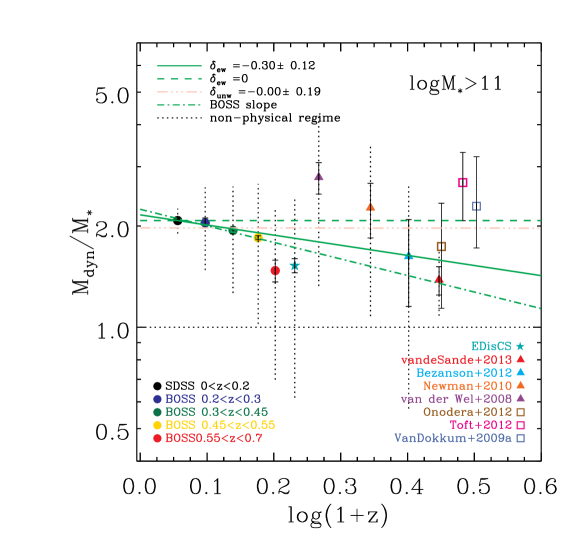
Figure 10.— Ratio between dynamical and stellar mass as a function of redshift extending up to $z\sim 2$ for galaxies with $\log$$M_{\star}$$/M_{\odot}>11$. Data samples from the literature with $z>0.7$ (see labels in the plot) have been added to the sample presented in Figure 8. The filled colored circles are the median $M_{\rm dyn}$/$M_{\star}$ ratios for the redshift bins of Figure 8. The filled star and triangles are the median $M_{\rm dyn}$/$M_{\star}$ ratios for each sample from the literature. Open squares are individual measurements for publications of only one object. The green solid line is the error-weighted linear fit to the median values plotted covering the full range in redshift $0.08<z<2.18$, whereas the pink line is the unweighted linear fit to the same points.The green dashed line is a fit with zero slope for comparison. The green dot-dashed line is the linear fit to our sample from Figure 8. The black dotted horizontal line indicates the non-physical regime of $M_{\rm dyn}/M_{\star}<1$ (below the line). Black dotted vertical lines indicate the standard deviation of the distribution at the given redshift.

In the past years a number of investigations have been dedicated to studying the dependence of dynamical to stellar mass ratios $M_{\rm dyn}$/$M_{\star}$ with galaxy mass in the local universe. There is a clear concordance that $M_{\rm dyn}$/$M_{\star}$ increases with galaxy mass. The origin of this trend remains controversial, however. It is still under debate whether this phenomenon is driven by dark matter fractions, variations of the IMF, non-homology of early-type systems or adiabatic contraction (Cappellari et al., 2006; Hyde & Bernardi, 2009a; Treu et al., 2010; Auger et al., 2010; Napolitano et al., 2010; Schulz et al., 2010; Dutton et al., 2011; Thomas et al., 2011; Cappellari et al., 2012; Conroy & van Dokkum, 2012; Dutton et al., 2012, 2013; van Dokkum & Conroy, 2012; Wegner et al., 2012; Conroy et al., 2013).

In this paper we study the evolution of the dynamical to stellar mass ratio of massive galaxies as a function of cosmic time. The extra dimension added with look-back time helps to break some of the degeneracies plaguing local studies, because we analyze a passively evolving galaxy population in a very small mass range (see Figure 7). In this case variations of the effective IMF due to mergers would be minor. We find that the dynamical to stellar mass ratio in massive galaxies of $M_{\star}\sim 2\times 10^{11}M_{\odot}$ decreases with increasing redshift at $>2\sigma$ significance over the redshift range $0.1<z<0.55$.

5.1. Comparison with high-redshift literature data

The relatively modest evolution of $M_{\rm dyn}/M_{\star}$ over the past seven billion years found here is well in line with other studies in the literature generally probing higher redshift and larger look-back times. The SDSS-III/BOSS data serve well in bridging galaxy properties from the distant with the local universe. In this section we will put those two data sets together comparing our results directly with the data at high redshift.

We collect public catalogs of structural parameters, stellar masses and stellar velocity dispersions from the EDisCS survey described in Saglia et al. (2010), for a sample of 154 cluster and field galaxies (41 field galaxies and 113 cluster galaxies) at median redshift $z\sim 0.7$. We derive dynamical masses as described in Section 3.4 using a variable $\beta(n)$ derived from EDisCS Sérsic indices and Equation 20 of Cappellari et al. (2006). We rescale sizes in kpc of Table 1 and 2 of Saglia et al. (2010) to our cosmology and stellar velocity dispersions are rescaled to $R_{\rm e}$ using Equation 2. Saglia et al. 2010 stellar masses, derived using Bruzual & Charlot (2003) models and a diet-Salpeter IMF (Bell & de Jong, 2001), are rescaled to a common Kroupa IMF (to match the IMF used for our local SDSS and BOSS sample), using a $-0.05\;$dex offset based on Table 2 of Bernardi et al. (2010). We select galaxies with $\log M/M_{\odot}>11$ resulting in 77 objects.

We collect $z>1$ data from van de Sande et al. (2013). These authors presented five new kinematic measurements of galaxies at $z>1.5$ and compiled a catalog of previous data in the range of $0.8<z<2.18$ (van der Wel et al., 2008; van Dokkum et al., 2009; Newman et al., 2010; Onodera et al., 2012; Toft et al., 2012; Bezanson et al., 2013a), for a total of 73 galaxies, 46 of which have $\log M/M_{\odot}>11$. The dynamical masses in van de Sande et al. (2013) were derived by using procedures similar to those described in Section 3.4, accounting for a variable $\beta(n)$, hence we only rescale them to our cosmology. Stellar masses, derived using Bruzual & Charlot (2003) models and a Chabrier (2003) IMF, were rescaled to a common Kroupa IMF using a $+0.05\;$dex offset based on Table 2 of Bernardi et al. (2010).

5.1.1 Stellar masses

Stellar masses derived with different population models may be different because of the different assumptions of stellar evolution in the models. Moreover, other assumptions regarding the star formation history, dust reddening and the assumed IMF all affect the final value of $M_{\star}$.

The variation in $M_{\star}$ is quantified in Pforr et al. (2012) as a function of population model, using Maraston (2005) and Bruzual & Charlot (2003) models, and as a function of the star formation history and IMF assumed in the models. We use their results for obtaining a homogeneous sample of $M_{\star}$.

As most of the galaxies in the $z>0.7$ sample studied here appear to be passive (van de Sande et al., 2013), we choose offsets from Table B4 of Pforr et al. (2012) derived for mock passive galaxies at $z=2$. As fitting setup we select the “wide BC03” with reddening included as adopted in the $z>0.7$ literature stellar masses, which gives an offset to Maraston (2005) based stellar masses of $0.13\;$dex. We note that the star-forming mocks show the same offset ($0.12\;$dex) for the “wide BC03” fitting setup, which is important as some of the galaxies in the sample might not be passive (see for instance the Bezanson et al. 2013a sample). We decrease the stellar masses of the $z>0.7$ sample by this amount. This offset is consistent with differences in stellar mass due to stellar population models found for BOSS galaxies (see Appendix of Maraston et al. 2013) and for galaxies in COSMOS (Ilbert et al., 2010).

It should be noted, however, that stellar masses also depend on the star formation history adopted for the SED fitting. Stellar masses of the $z>0.7$ sample were obtained assuming an exponentially decaying star formation history. However, galaxies at those redshift may be better modeled with an exponentially increasing star formation history (Maraston et al., 2010), which would give higher stellar masses by $\sim 0.2\;$dex compensating the offset applied here. Ideally the full sample should be modeled self-consistently, but the photometry of the $z>0.7$ sample is not available to us. We will therefore discuss final results based on both with and without the offset of $0.13\;$dex in stellar mass.

5.1.2 Evolution of $M_{\rm dyn}$/$M_{\star}$

Figure 10 presents the evolution of the dynamical to stellar mass ratio as a function of redshift for the redshift interval $0.08<z<2.18$. The SDSS-II and SDSS-III/BOSS data of the present study is combined with the high-$z$ samples discussed in the previous section. The $0.13\;$dex offset between the stellar masses of the low- and high-$z$ samples has been applied. The symbols plotted are the median values of both $M_{\rm dyn}/M_{\star}$ and $z$. Error bars are standard errors, while the dotted lines indicate the standard deviation of the distribution at the given redshift.

The high-$z$ sample is consistent with the trend of decreasing $M_{\rm dyn}/M_{\star}$, even though the scatter at $z>1$ is large. The BOSS data at intermediate redshifts clearly drives this relationship, because of the large scatter in the data at high redshift. By fitting the data over the full redshift range of $0.08<z<2.18$ as shown in Figure 10 and including the error bars in the fit, we find $M_{\rm dyn}$/$M_{\star}$$\propto(1+z)^{-0.30\pm 0.12}$ (where $\delta_{\rm ew}$ is the slope, and “ew” stands for error-weighted fit). This slope is slightly shallower but well consistent with the value derived in this work from the SDSS-II and SDSS-III/BOSS data alone (dot-dashed line, see Figure 8). Most importantly, the statistical significance for the presence of a negative slope is $>2\sigma$ also in this case. This further reinforces the evidence for a decrease in $M_{\rm dyn}/M_{\star}$ with increasing redshift.

Error weighting the fit could potentially bias our results towards the BOSS sample, where the statistic is much larger and errors on the mean values are smaller. Therefore, we repeated the same procedure above using an equal weighting for all the points. This is shown by the pink three-dot-dashed line in Figure 10 (where $\delta_{\rm unw}$ is the slope, ans “unw” stands for unweighted fit). In this case we find almost no evolution as we could easily expect. Given the large uncertainties and the low statistic in the high-z sample applying a different weight to the BOSS sample would be preferable. A larger sample of high-redshift data would be helpful to constrain the evolution $M_{\rm dyn}$/$M_{\star}$ ratio over a redshift range wider than that of BOSS.

Figure 11 shows the case in which the offset to the stellar masses has not been applied. As the correction implied a decrease of stellar masses in the high-$z$ sample, the decrease of $M_{\rm dyn}/M_{\star}$ with increasing redshift becomes even steeper and the statistical significance increases to $>4\sigma$.

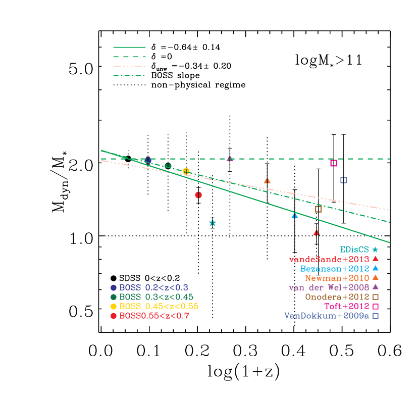
Figure 11.— Same as Figure 10 but without correction for offset in stellar masses due to differences in stellar population modeling (see text for details).

5.2. Decreasing dark matter fraction due to size growth

The increase of $M_{\rm dyn}$ with cosmic time is most plausibly caused by an increase of dark matter fraction within the effective radius. This increase can be well understood through size growth, which causes an increase of the dark matter fraction within an increasing effective radius (van de Sande et al., 2013). Indeed simulations show that the addition of stars in the outskirts of galaxies following the minor merger scenario can lead to an increased measured dark matter fraction by $\sim 80$% (Johansson et al., 2012; Hilz et al., 2012) because more area with larger dark matter fraction is also included within $R_{\rm e}$ (Hilz et al., 2013; Hopkins et al., 2009). Also Toft et al. (2012) studying galaxies at $z\sim 2$ with available kinematics suggest that the low dark matter fraction of galaxies at $z\sim 2$ is in favor of the merger scenarios which can redistribute dark matter within $R_{\rm e}$ (Boylan-Kolchin et al., 2005; Oser et al., 2012).

The steady increase of the dark matter fraction in the centers of massive galaxies with time further implies that massive galaxies in the local universe must contain some dark matter within their half-light radii, even if they are baryon dominated. This is consistent with recent dynamical modeling of nearby galaxies implying dark matter fractions of $16-28\%$ (Thomas et al., 2011; Cappellari et al., 2013b) as well as simulations predicting dark matter fractions of $18-38\%$ (Naab et al., 2007, and references therein).

6. Conclusions

We study the redshift evolution of the dynamical properties of $\sim 180,000$ galaxies from the SDSS-III/BOSS survey. We examine the redshift evolution of luminous, massive galaxies ($M\sim 2\times 10^{11}M_{\odot}$) at fixed stellar or dynamical mass for the first time for such a large sample size.

Despite the relatively low $S/N$ of BOSS spectra, it is possible to measure $\sigma$ for a large sample of galaxies in the range $0.2\leq z\leq 0.7$ with a typical error $\leq$ 30%. Stellar velocity dispersions are adopted from Thomas et al. (2013).

At BOSS redshifts effective radii are barely resolved in the SDSS imaging, and higher resolution images would be needed, which are not available for the whole sample. Therefore, we used a sub-sample of BOSS galaxies for which HST photometry is available as part of the COSMOS survey (Masters et al., 2011). We derived a correction to physical effective radii derived from SDSS photometry by dividing our sample in four redshift bins and searching for correlations between the ratio of the SDSS $R_{\rm e}$ and HST/COSMOS $R_{\rm e}$ as a function of the SDSS $R_{\rm e}$.

We then derive dynamical mass estimates by means of a simple virial mass estimator based on galaxy effective radius and velocity dispersions within the effective radius. These total dynamical masses are compared to the total stellar masses derived by Maraston et al. (2013) studying the redshift evolution of the galaxy parameters effective radius, stellar velocity dispersion, and dynamical to stellar mass ratio $M_{\rm dyn}/M_{\star}$. We complement the SDSS-III/BOSS sample with local early-type galaxies from SDSS-II after matching their mass distributions, so that our study covers the redshift range $0.1<z<0.55$.

To account for the effects of the so-called progenitor bias we compare the galaxy ages in each redshift bin and remove those galaxies from the low-$z$ sample whose ages after evolution to the highest redshift bin would be lower than a given age threshold. As result we study a sample of passively evolving galaxies within a relatively narrow mass range about $M\sim 2\times 10^{11}M_{\odot}$ (for a Kroupa IMF).

We find a moderate size evolution at the $\sim 1.5\sigma$ level, with galaxy radii decreasing with increasing redshift in agreement with previous results and model predictions (Oser et al. 2012; but better with Nipoti et al. 2012, Khochfar & Silk 2006 or Hopkins et al. 2009). We further observe a mild, but significant ($>2\sigma$), evolution in velocity dispersion of $\sigma$ increasing with increasing redshift. The evolution of stellar velocity dispersion and effective radius together combine to an evolution of the dynamical to stellar mass ratio, such that $M_{\rm dyn}/M_{\star}$ increases with decreasing redshift at $>2\sigma$ significance. We emphasize that we are probing a variation of stellar kinematics within the effective radius, hence this evolution is caused by a change of dynamical mass within $1R_{\rm e}$, even though total masses are compared.

The major sources for random and systematic errors are the size correction and the calculation of dynamical mass through the virial estimator. To assess random and systematic errors in the redshift evolution of these galaxy parameters we perform Monte Carlo simulations perturbing the size correction, as well as the structural dependent constant of proportionality of the virial mass estimator within their errors. In the appendix we present several additional tests on the impact of the progenitor bias correction, of aperture effects, of a possible redshift dependence of the virial constant, and of a mismatch in mass distribution between the local and the high-$z$ galaxy samples. We show that, while the details and the exact strengths of the correlations between $R_{\rm e}$, $\sigma$, and $M_{\rm dyn}/M_{\star}$ with redshift vary, the general detection of a redshift evolution of these parameters is robust against the systematic uncertainties from these procedures.

Finally, we extend the present study to higher redshifts by combining our sample with high-redshift literature data (Saglia et al., 2010; van de Sande et al., 2013) so that we cover the full redshift range from $z\sim 0.1$ to $z\sim 2$. The high-$z$ sample is consistent with the trend of decreasing $M_{\rm dyn}/M_{\star}$, even though the scatter at $z>1$ is large. By fitting the data over the full redshift range we find $M_{\rm dyn}$/$M_{\star}$$\propto(1+z)^{-0.30\pm 0.12}$. This slope is slightly shallower but well consistent with the value derived in this work from the SDSS-II and SDSS-III/BOSS data alone. Our results are clearly driven by the BOSS sample in which the large number statistics allows us to have smaller uncertainties on average quantities as a function of redshift and help to identify and quantify redshift-dependent trends. Most importantly, the evidence for a decrease of $M_{\rm dyn}/M_{\star}$ with increasing redshift is reinforced further at $>2\sigma$ statistical significance, although a larger sample of high-redshift data would be helpful to constrain the evolution $M_{\rm dyn}$/$M_{\star}$ ratio over a redshift range wider than that of BOSS.

We discuss that the increase of $M_{\rm dyn}$ with cosmic time is most plausibly caused by an increase of dark matter fraction within the effective radius. This evolution can be well understood through the size growth, which causes an increase of the dark matter fraction within an increasing effective radius as also predicted by galaxy formation simulations based on minor merger driven mass growth. Major mergers could also result in an evolution of $M_{\rm dyn}$/$M_{\star}$, but of smaller amount; however, with our data we cannot constrain any difference between minor and major mergers. Finally it is interesting to note that the steady increase of the dark matter fraction in the centers of massive galaxies with time further implies that massive galaxies in the local universe must contain some dark matter within their half-light radii, even if they are baryon dominated.

Appendix A A.  Stellar masses from one effective radius aperture magnitudes

The dynamical mass obtained using the virial mass estimator (see Section 3.4) is based on stellar kinematics within an aperture of 1 effective radius and scaled to total dynamical mass via equation 3. This quantity is compared with the total stellar mass from Maraston et al. (2013) based on cmodelMag magnitudes. Hence both dynamical and stellar masses are total masses, which ensures a consistent comparison.

Still, the total dynamical mass is derived from observations within the effective radius, while the stellar mass comes from the total stellar light. We explore therefore the possible presence of a systematic effect from the different apertures in which kinematics and stellar populations have been measured. In this test we compare $M_{\star}$ derived from modelmag (rescaled to cmodelmag) and $M_{\star}$ from aperture magnitudes within $R_{\rm e}$ (rescaled to cmodelmag), for a sub-sample of 1,000 galaxies randomly selected among the BOSS sample to assess differences between the two quantities. We derive magnitudes within the two apertures closest to the effective radius of each galaxy in $i$-band (the same $R_{\rm e}$ we used for $M_{\rm dyn}$ determination) and we interpolate magnitudes to derive the value we would have at $R_{\rm e}$ in each band. Aperture magnitudes are then rescaled to cmodelmag in $i$-band to make sure that any difference on the resulting stellar mass comes from differences in the $M/L$ ratio and SED shape.

In detail, we collect our reference (circularized) $i$-band radii following Section 3.2.1. We estimate aperture magnitudes following the step described at http://www.sdss3.org/dr8/algorithms/magnitudes.php_photo_profile through a casjob query. We first derive nprof, from the PhotoObjAll table, which gives us the number of annuli (concentric circles) for which there is a measurable signal in $u,g,r,i,z-$ bands. From the photoProfile table, where azimuthally-averaged radial profiles of SDSS photo objects are listed, we create circular aperture magnitudes from profMean (the mean surface brightness within the annuli) and their errors (profErr) which are both in $nanomaggies/arcsec^{2}$. Quantities are then converted from nanomaggie following http://www.sdss3.org/dr8/algorithms/magnitudes.php_nmgy. The bin keyword gives the annuli from which the profile was derived (from 0 to 14) and band gives the selected $u,g,r,i,z-$ band (from 0$-$4). We integrate profMean values within each of the two annuli close to the circularized $i$-band effective radii. In our query we impose that magnitudes are only calculated when fluxes within the aperture in nanomaggies are positive. We also tested whether the number of available bins for each galaxy is smaller or equal to the requested aperture. The final sample for which we are able to derive aperture magnitudes reduces to 604 galaxies due to the quality of the $u$-band data. Magnitudes in the two annuli close to $R_{\rm e}$ are then linearly interpolated to derive the value at $R_{\rm e}$.

The histogram of the resulting difference between $M_{\star}$ obtained using modelmag rescaled to cmodelmag and 1$R_{\rm e}$ aperture magnitudes rescaled to cmodelmag is shown in Figure 12. The difference is $\sim-0.08\;$dex in log (25%). The slightly redder populations in the more central aperture photometry (1$R_{\rm e}$ aperture magnitude colors are redder than modelmag colors) leads to slightly higher $M/L$ ratios and hence slightly higher masses. However, this result suggests that the systematic offset is small. Our $M_{\rm dyn}$/$M_{\star}$ ratios are always above 0.08 dex, so by rescaling Maraston et al. (2013) stellar masses there is no risk that $M_{\star}$ exceeds $M_{\rm dyn}$, which would be unphysical. We also note that the difference between $M_{\star}$ obtained using modelmag rescaled to cmodelmag and 1$R_{\rm e}$ aperture magnitudes rescaled to cmodelmag does not depend on redshift (the redshift variation is $\sim 0.01$ dex, of the order of the uncertainties on $M_{\star}$). Therefore, our analysis, focused on redshift variations, is not affected.

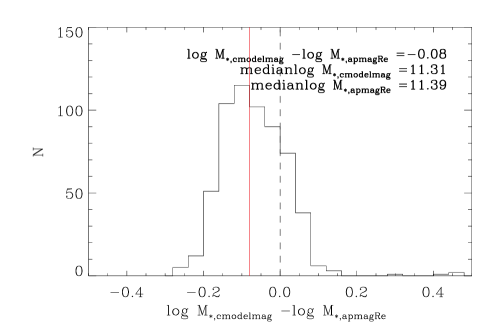
Figure 12.— Comparison between stellar masses derived from modelmag and aperture magnitudes within $1R_{\rm e}$ both rescaled to $i$-band cmodelmag to give total mass. The median difference between the two masses is $\sim-0.08\;$dex (25%, continuous-red line). Galaxies are redder inside the effective radius leading to higher $M/L$ ratios and hence larger total mass (when scaled to total light).

Appendix B B.  Impact of unresolved multiple systems in the SDSS images

The presence of unresolved multiple systems in the SDSS images could potentially introduce spurious trends in the measured evolution of sizes, dynamical masses and stellar masses. In this Appendix we study their influence in our size calibration and in the stellar mass estimation.

Masters et al. (2011) found that the 23% of the COSMOS/BOSS sub-sample shows two components in the COSMOS images, which are unresolved in the SDSS images. We further investigate this, considering only objects showing a size overestimation after our size calibration.

Figure 13, left panel, shows the distribution of the ratio between corrected sizes and COSMOS sizes for 206 objects part of the COSMOS/BOSS sub-sample in the redshift range $0.2\lesssim z\lesssim 0.7$. Those include both single objects (163 galaxies, blue filled histogram) and unresolved multiple systems (43 galaxies, red empty histogram). Our size correction allows to adjust most of the unresolved multiple systems, resulting in a distribution similar to that of the single objects but with a tail at larger ratios. A closer look at the catalog of Masters et al. (2011) (available at http://www.icg.port.ac.uk/$\sim$mastersk/BOSSmorphologies/) shows that when the secondary object in the system is very faint, its effect on the radius measured by the SDSS pipeline seems to be reduced, resulting in sizes not massively overestimated.

We estimate the further correction we have to apply to unresolved multiple systems, considering the 12 objects ($\sim 6$% of our COSMOS/BOSS sub-sample) which are in the tail, as shown by the green histogram in the central panel of Figure 13. Although the effect of the multiple systems is likely to be redshift dependent, the small sample we are considering here does not allow a division in redshift bins. Moreover, due to the small statistic, we make use the full distribution to derive the correction factor for sizes, which ranges between a factor 2 and 3.

Similarly to sizes, stellar masses of unresolved multiple systems could be biased too. We use the same 12 galaxies with overestimated corrected sizes to assess this effect. Under the assumption that our galaxies are passively evolving, we can estimate the bias in the stellar mass from the ratio of the fluxes of the two components resolved by the COSMOS imaging. If galaxies were not passively evolving the luminosity would be diluted but our conclusions would not change appreciably. Fluxes were derived from the MAG_AUTO listed in the Zurich Structure & Morphology Catalog v1.0 available at http://irsa.ipac.caltech.edu/data/COSMOS/datasets.html and described in Section 3.2.2. Given that we do not have accurate information about the redshifts of the two systems we used as estimate the parent magnitudes and not absolute magnitudes. Two objects are discarded because, by visual inspection, their separation looked large enough for each of them to be considered two separated sources, suggesting a smaller bias in the SDSS magnitudes used in the stellar mass calculation (separation $>2\times{\rm FWHM_{seeing}}$). This retains 10 objects ($\sim$ 5% of the total sample of COSMOS/BOSS galaxies). The distribution of the relative flux ratio of the objects which are resolved in the COSMOS images, $(I_{1}+I_{2})/I_{1}$, is shown in the central panel of Figure 13, where $I_{1}$ is the flux of the primary brightest object in COSMOS, and $I_{2}$ is the flux of the secondary objects within 2 times the typical FWHM of the SDSS seeing ($\sim$1$\farcs$1, see Section 3.2.1 for details). The average correction factor for fluxes (or masses) is about 1.54.

Although stellar velocity dispersions, to some extent, can be biased too, the estimation of this effect is not trivial and cannot be done without additional spectroscopy, therefore we disregard any possible biases to stellar velocity dispersions due to unresolved multiple in our analysis.

Right panel of Figure 13 compares the flux (i.e., mass) correction with the size correction for final sample of 10 unresolved multiple systems used here. Typical size corrections range between a factor 2 and 3, whereas the flux (mass) correction is much smaller ($\sim 1.54$) as shown by the dotted lines parallel to the continuous one-to-one relation in a manner which does not seem to change with redshift (but the statistic is too small to make strong statements).

We finally apply the redshift independent size and mass corrections to a randomly selected 6% sub-sample of BOSS galaxies and analyze the effects on our results. The corrections were also included in our Monte Carlo estimation of systematic errors. The resulted combined effect on sizes and masses is negligible and our results do not change substantially considering this additional correction or not (if not improve them of about $<2$% ). Figures 8, 9, 10 and 11 and Table 2 include this additional correction.

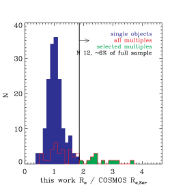
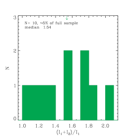
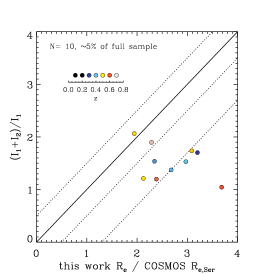
Figure 13.— Left Panel: Distribution of the ratio between our corrected SDSS $R_{\rm e}$ and COSMOS $R_{\rm e,Ser}$ (blue filled histogram) and distribution of unresolved multiple systems (red empty histogram). The green filled histogram shows the sample of unresolved multiple systems which were used to study the impact of these objects on our results. Central Panel: Distribution of the ratio between the fluxes (masses) of the two components which are resolved in the COSMOS photometry. Right Panel: Comparison between the size excess and the flux (mass) excess in our sample of 10 multiple systems coded as a function of redshift. By using sizes from SDSS we tend to overestimate sizes of a factor 2 to 3 and fluxes of a factor $\sim$1.54. The continuous line corresponds to the one-to-one relation and dotted lines show the intercepts $\pm$0.5 and 1.3x.

Appendix C C.  Tests on evolution: BOSS sample, and use of constant or redshift dependent $\beta$

In this Appendix we show that our results do not change when we analyze scaling relations only using the BOSS sample. Table 3 (case in which $\beta$ is assumed constant with redshift) shows that the trends we find in Section 4 are maintained, although the significance of the results is reduced. Errors from the Monte Carlo simulations for the BOSS sample are $50-60$% larger than using the combined sample of local and BOSS data (see Figure 8 and Table 2). The significance is particularly reduced for the size evolution. We conclude that the addition of the local early-type sample does not affect our results but helps constraining the fits. Results are summarized in Table 3.

Sérsic indices from HST photometry are available as part of the BOSS/COSMOS sub-sample (see Section 3.4.1).

This allows us to assess the effect of a redshift-dependent $\beta(n)$ parameter, through our Monte Carlo simulations. The results of this test are shown in Figure 14 and summarized in Table 3 (columns with $z$-variable $\beta$). By using a redshift dependent $\beta$ on Equation 3 for $M_{\rm dyn}$, the evolution of the $M_{\rm dyn}$/$M_{\star}$ ratio becomes more significant than using a constant $\beta$ (more conservative results). The difference on the slopes, however, is very small ($\sim 10$%) suggesting that $\beta(n)$ does not strongly evolve in the BOSS redshift range and any possible variation would not affect our results. Table 3 summarizes the comparison between a redshift dependent or a constant $\beta$.

The analysis above can be done only for the COSMOS/BOSS sample, because structural parameters are measured in a similar way and on the same images.

We use the photometric catalog of Simard et al. (2011) for SDSS local galaxies to compare structural parameters (i.e., Sérsic indices) of the local and BOSS/COSMOS sample. Simard et al. (2011) presented new structural parameters from both single Sérsic fits and bulge-to-disk decomposition on the full DR7 sample in $g$ and $r$-band. For our tests we chose data from single Sérsic fit to be consistent with COSMOS (in particular around the transition redshift $z\sim 0.2$).

The Simard et al. (2011) and COSMOS catalogs have a limited number of objects in common. For $n<4$ we found a fair agreement between structural parameters in the two catalog, whereas for $n>4$, Simard et al. (2011) Sérsic indices are larger than COSMOS ones. By using median Simard et al. (2011) Sérsic indices for our early-types sample we reproduce the commonly used $\beta(n)\sim 5$ for local galaxies. Sérsic indices of the two samples probably differ because they were derived with different images and approaches and there is no clear correction to be applied to this.

For this reason in our analysis we do not combine information about the Sérsic indices from Simard et al. (2011) and COSMOS. Instead we adopt the redshift independent $\beta$ of the BOSS galaxies also for the SDSS sample.

An explanation of these differences is beyond the scope of this paper.

Table 3Fitting parameters for the BOSS sample between $0.2<z<0.55$, in which the progenitor-bias correction is applied.

	$M_{\star}$				$M_{\rm dyn}$
Parameter	constant $\beta$		$z$-variable $\beta$		constant $\beta$		$z$-variable $\beta$
	slope	z=0	slope	z=0	slope	z=0	slope	z=0
$R_{\rm e}$	$-0.46\pm 0.56$	$0.76\pm 0.09$	$-0.46\pm 0.55$	$0.76\pm 0.09$	$-0.32\pm 0.47$	$0.73\pm 0.08$	$-0.28\pm 0.46$	$0.73\pm 0.08$
$\sigma_{\rm e}$	$0.12\pm 0.04$	$2.36\pm 0.006$	$0.12\pm 0.04$	$2.36\pm 0.006$	$0.20\pm 0.13$	$2.35\pm 0.02$	$0.25\pm 0.13$	$2.34\pm 0.02$
$M_{\rm dyn}/M_{\star}$	$-0.53\pm 0.48$	$0.36\pm 0.08$	$-0.78\pm 0.52$	$0.40\pm 0.08$	$-0.77\pm 0.35$	$0.41\pm 0.06$	$-0.92\pm 0.37$	$0.43\pm 0.06$

Notes. — Uncertainties on each parameter are $1\sigma$ errors derived from Monte Carlo simulations. The relation we fitted for $R_{\rm e}$ is $\log R_{\rm e}=\log R_{\rm e,0}+\beta(1+z)$, for $\sigma_{\rm e}$ is $\log\sigma_{\rm e}=\log\sigma_{\rm e,0}+\gamma(1+z)$, and for $M_{\rm dyn}/M_{\star}$ is $\log(M_{\rm dyn}/M_{\star})=\log(M_{\rm dyn}/M_{\star})_{0}+\delta(1+z)$ .

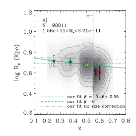
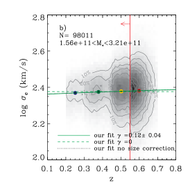
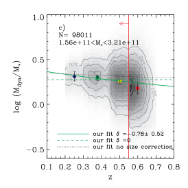
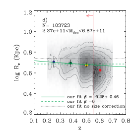
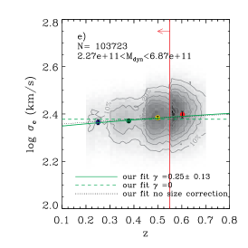
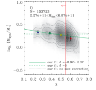
Figure 14.— Same as Figure 8 but for the SDSS-III/BOSS sample only and with a redshift dependent $\beta$ (see Equation 3).

Appendix D D.  Tests on evolution: local early-types & BOSS samples without progenitor bias correction

In Section 3.6 we discuss the correction for progenitor bias applied in this work. To study the impact of this correction on our analysis, we have performed a re-analysis for a sample without progenitor bias correction. Figure 15 shows the redshift evolution of the galaxy parameters size, stellar velocity dispersion and $M_{\rm dyn}$/$M_{\star}$ without progenitor bias correction. The fit parameters are given in Table LABEL:tab:fitsnobias. Comparing to Figure 8 and Table LABEL:tab:fits in the main text it can be seen that generally the results are fairly stable against the progenitor-bias correction, significant evolution with redshift is still detected for all three parameters. We infer that the main conclusions of this paper do not critically depend on the progenitor bias correction.

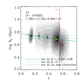
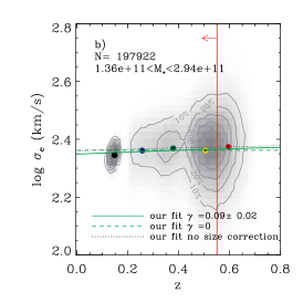
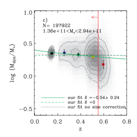
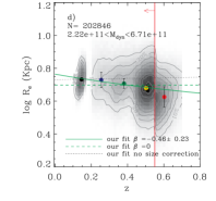
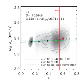
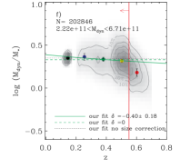
Figure 15.— Same as Figure 8 but no correction for progenitor bias.

Table 4Fitting parameters for the redshift evolution of galaxy parameters between $0.1\leq z\leq 0.55$ without progenitor bias correction

	$M_{\star}$		$M_{\rm dyn}$
Parameter	slope	zero point	slope	zero point
$R_{\rm e}$	$-0.50\pm 0.28$	$0.78\pm 0.04$	$-0.46\pm 0.23$	$0.76\pm 0.03$
$\sigma_{\rm e}$	$0.09\pm 0.02$	$2.36\pm 0.00$	$0.13\pm 0.06$	$2.35\pm 0.01$
$M_{\rm dyn}/M_{\star}$	$-0.54\pm 0.24$	$0.40\pm 0.03$	$-0.40\pm 0.18$	$0.38\pm 0.02$

Notes. — Uncertainties on each parameter are $1\sigma$ errors derived from Monte Carlo Simulations. The relation we fitted for $R_{\rm e}$ is $\log R_{\rm e}=\log R_{\rm e,0}+\beta(1+z)$, for $\sigma_{\rm e}$ is $\log\sigma_{\rm e}=\log\sigma_{\rm e,0}+\gamma(1+z)$, and for $M_{\rm dyn}/M_{\star}$ is $\log(M_{\rm dyn}/M_{\star})=\log(M_{\rm dyn}/M_{\star})_{0}+\delta(1+z)$.

Appendix E E.  Tests on evolution: stellar mass distribution of local early-types & BOSS galaxies

As described in Section 3.5 we homogenize the stellar mass distributions between the local sample from SDSS-II and the high-$z$ sample from SDSS-III/BOSS by selecting a local sub-sample that matches the mass distribution of the BOSS sample. In this Appendix we present a re-analysis in which we do not apply this homogenization. The distributions of stellar masses, dynamical masses, stellar velocity dispersions, and effective radii are shown in Figure 16. Figure 17 shows the redshift evolution of the galaxy parameters size, stellar velocity dispersion and $M_{\rm dyn}$/$M_{\star}$, the fit parameters are summarized in Table LABEL:tab:fitsnomassdistrib. It can be seen that our finding of redshift evolution remains intact for all three parameters, and the significance of the slopes only changes slightly.

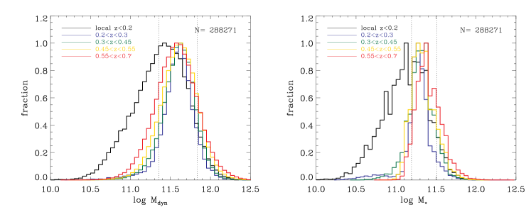
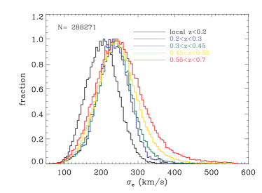
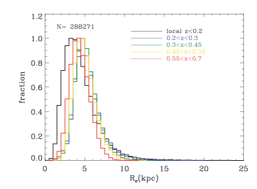
Figure 16.— Same as Figure 7 but no homogenization between the mass distributions of the local sample from SDSS-II and the sample from SDSS-III/BOSS.

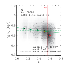
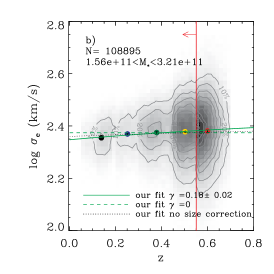
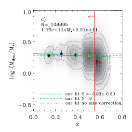
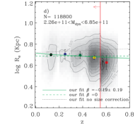
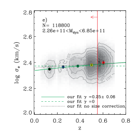
Figure 17.— Same as Figure 8 but no homogenization between the mass distributions of the local sample from SDSS-II and the sample from SDSS-III/BOSS.

Table 5Fitting parameters for the redshift evolution of galaxy parameters between $0.1\leq z\leq 0.55$ without matching mass distributions between the local SDSS-II and the SDSS-III/BOSS samples

	$M_{\star}$		$M_{\rm dyn}$
Parameter	slope	zero point	slope	zero point
$R_{\rm e}$	$-0.43\pm 0.27$	$0.76\pm 0.04$	$-0.19\pm 0.19$	$0.72\pm 0.03$
$\sigma_{\rm e}$	$0.18\pm 0.02$	$2.35\pm 0.00$	$0.25\pm 0.06$	$2.34\pm 0.01$
$M_{\rm dyn}/M_{\star}$	$-0.23\pm 0.23$	$0.32\pm 0.03$	$-0.36\pm 0.14$	$0.34\pm 0.02$

Notes. — Uncertainties on each parameter are $1\sigma$ errors derived from Monte Carlo simulations. The relation we fitted for $R_{\rm e}$ is $\log R_{\rm e}=\log R_{\rm e,0}+\beta(1+z)$, for $\sigma_{\rm e}$ is $\log\sigma_{\rm e}=\log\sigma_{\rm e,0}+\gamma(1+z)$, and for $M_{\rm dyn}/M_{\star}$ is $\log(M_{\rm dyn}/M_{\star})=\log(M_{\rm dyn}/M_{\star})_{0}+\delta(1+z)$.

References

- Abazajian et al. (2009) Abazajian, K. N., Adelman-McCarthy, J. K., Agüeros, M. A., et al. 2009, ApJS, 182, 543
- Ahn et al. (2012) Ahn, C. P., Alexandroff, R., Allende Prieto, C., et al. 2012, ApJS, 203, 21
- Aihara et al. (2011) Aihara, H., Allende Prieto, C., An, D., et al. 2011, ApJS, 193, 29
- Anderson et al. (2012) Anderson, L., Aubourg, E., Bailey, S., et al. 2012, MNRAS, 427, 3435
- Auger et al. (2010) Auger, M. W., Treu, T., Bolton, A. S., et al. 2010a, ApJ, 724, 511
- Auger et al. (2010) Auger, M. W., Treu, T., Gavazzi, R., et al. 2010b, ApJ, 721, L163
- Beifiori et al. (2012) Beifiori, A., Courteau, S., Corsini, E. M., & Zhu, Y. 2012, MNRAS, 419, 2497
- Beifiori et al. (2011) Beifiori, A., Maraston, C., Thomas, D., & Johansson, J. 2011, A&A, 531, A109
- Bell & de Jong (2001) Bell, E. F., & de Jong, R. S. 2001, ApJ, 550, 212
- Belli et al. (2014) Belli, S., Newman, A. B., & Ellis, R. S. 2014, ApJ, 783, 117
- Bender (1990) Bender, R., 1990, A&A, 229, 441
- Bender et al. (1992) Bender, R., Burstein, D., & Faber, S. M. 1992, ApJ, 399, 462
- Bender et al. (1993) Bender, R., Burstein, D., & Faber, S. M. 1993, ApJ, 411, 153
- Bender et al. (1994) Bender, R., Saglia, R. P., & Gerhard, O. E. 1994, MNRAS, 269, 785
- Bender et al. (1998) Bender, R., Saglia, R. P., Ziegler, B., et al. 1998, ApJ, 493, 529
- Bernardi et al. (2010) Bernardi, M., Shankar, F., Hyde, J. B., et al. 2010, MNRAS, 404, 2087
- Bernardi (2009) Bernardi, M. 2009, MNRAS, 395, 1491
- Bernardi et al. (2008) Bernardi, M., Hyde, J. B., Fritz, A., et al. 2008, MNRAS, 391, 1191
- Bernardi et al. (2007) Bernardi, M., Hyde, J. B., Sheth, R. K., Miller, C. J., & Nichol, R. C. 2007, AJ, 133, 1741
- Bernardi et al. (2006) Bernardi, M., Sheth, R. K., Nichol, R. C., et al. 2006, AJ, 131, 2018
- Bernardi et al. (2003) Bernardi, M., Sheth, R. K., Annis, J., et al. 2003, AJ, 125, 1817
- Bertin et al. (2002) Bertin, G., Ciotti, L., Del Principe, M., 2002, A&A, 386, 149
- Bezanson et al. (2009) Bezanson, R., van Dokkum, P. G., Tal, T., et al. 2009, ApJ, 697, 1290
- Bezanson et al. (2013a) Bezanson, R., van Dokkum, P., van de Sande, J., Franx, M., & Kriek, M. 2013a, ApJ, 764, L8
- Bezanson et al. (2013b) Bezanson, R., van Dokkum, P. G., van de Sande, J., et al. 2013, ApJ, 779, L21
- Blanton et al. (2011) Blanton, M. R., Kazin, E., Muna, D., Weaver, B. A., & Price-Whelan, A. 2011, AJ, 142, 31
- Bolton et al. (2012a) Bolton, A. S., Brownstein, J. R., Kochanek, C. S., et al. 2012a, ApJ, 757, 82
- Bolton et al. (2012b) Bolton, A. S., Schlegel, D. J., Aubourg, É., et al. 2012b, AJ, 144, 144
- Bolton et al. (2008) Bolton, A. S., Burles, S., Koopmans, L. V. E., et al. 2008, ApJ, 682, 964
- Bolton et al. (2006) Bolton, A. S., Burles, S., Koopmans, L. V. E., Treu, T., & Moustakas, L. A. 2006, ApJ, 638, 703
- Bolzonella et al. (2010) Bolzonella, M., Kovač, K., Pozzetti, L., et al. 2010, A&A, 524, A76
- Boylan-Kolchin et al. (2005) Boylan-Kolchin, M., Ma, C.-P., Quataert, E., 2005, MNRAS, 362, 184
- Brownstein et al. (2012) Brownstein, J. R., Bolton, A. S., Schlegel, D. J., et al. 2012, ApJ, 744, 41
- Bruzual & Charlot (2003) Bruzual, G., & Charlot, S. 2003, MNRAS, 344, 1000
- Buitrago et al. (2008) Buitrago, F., Trujillo, I., Conselice, C. J., et al. 2008, ApJ, 687, L61
- Caon et al. (1993) Caon, N., Capaccioli, M., D’Onofrio, M., 1993, MNRAS, 265, 1013
- Cappellari et al. (2006) Cappellari, M., Bacon, R., Bureau, M., et al. 2006, MNRAS, 366, 1126
- Cappellari et al. (2009) Cappellari, M., di Serego Alighieri, S., Cimatti, A., et al. 2009, ApJ, 704, L34
- Cappellari & Emsellem (2004) Cappellari, M., Emsellem, E., 2004, PASP, 116, 138
- Cappellari et al. (2013a) Cappellari, M., McDermid, R. M., Alatalo, K., et al. 2013a, MNRAS, 432, 1862
- Cappellari et al. (2013b) Cappellari, M., Scott, N., Alatalo, K., et al. 2013b, MNRAS, 432, 1709
- Cappellari et al. (2012) Cappellari, M., McDermid, R. M., Alatalo, K., et al. 2012, Nature, 484, 485
- Carrasco et al. (2010) Carrasco, E. R., Conselice, C. J., & Trujillo, I. 2010, MNRAS, 405, 2253
- Cenarro & Trujillo (2009) Cenarro, A. J., Trujillo, I., 2009, ApJ, 696, L43
- Chabrier (2003) Chabrier, G. 2003, ApJ, 586, L133
- Chen et al. (2012) Chen, Y.-M., Kauffmann, G., Tremonti, C. A., et al. 2012, MNRAS, 421, 314
- Cimatti et al. (2008) Cimatti, A., Cassata, P., Pozzetti, L., et al. 2008, A&A, 482, 21
- Cimatti et al. (2012) Cimatti, A., Nipoti, C., & Cassata, P. 2012, MNRAS, 422, L62
- Ciotti et al. (1996) Ciotti, L., Lanzoni, B., Renzini, A., 1996, MNRAS, 282, 1
- Conroy & van Dokkum (2012) Conroy, C., & van Dokkum, P. G. 2012, ApJ, 760, 71
- Conroy et al. (2013) Conroy, C., Dutton, A. A., Graves, G. J., Mendel, J. T., & van Dokkum, P. G. 2013, ApJ, 776, L26
- Daddi et al. (2005) Daddi, E., Renzini, A., Pirzkal, N., et al. 2005, ApJ, 626, 680
- Damjanov et al. (2009) Damjanov, I., McCarthy, P. J., Abraham, R. G., et al. 2009, ApJ, 695, 101
- Damjanov et al. (2013) Damjanov, I., Chilingarian, I., Hwang, H. S., & Geller, M. J. 2013, ApJ, 775, L48
- Dawson et al. (2013) Dawson, K. S., Schlegel, D. J., Ahn, C. P., et al. 2013, AJ, 145, 10
- de Zeeuw et al. (2002) de Zeeuw, P. T., Bureau, M., Emsellem, E., et al. 2002, MNRAS, 329, 513
- Djorgovski & Davis (1987) Djorgovski, S., Davis, M., 1987, ApJ, 313, 59
- Dressler et al. (1987) Dressler, A., Lynden-Bell, D., Burstein, D., et al. 1987, ApJ, 313, 42
- Dutton et al. (2011) Dutton, A. A., Conroy, C., van den Bosch, F. C., et al. 2011, MNRAS, 416, 322
- Dutton et al. (2013) Dutton, A. A., Macciò, A. V., Mendel, J. T., & Simard, L. 2013, MNRAS, 432, 2496
- Dutton et al. (2012) Dutton, A. A., Mendel, J. T., Simard, L., 2012, MNRAS, 422, L33
- Eisenstein et al. (2001) Eisenstein, D. J., Annis, J., Gunn, J. E., et al. 2001, AJ, 122, 2267
- Eisenstein et al. (2011) Eisenstein, D. J., Weinberg, D. H., Agol, E., et al. 2011, AJ, 142, 72
- Franx et al. (2008) Franx, M., van Dokkum, P. G., Schreiber, N. M. F., et al. 2008, ApJ, 688, 770
- Fukugita et al. (1996) Fukugita, M., Ichikawa, T., Gunn, J. E., et al. 1996, AJ, 111, 1748
- Gerhard et al. (2001) Gerhard, O., Kronawitter, A., Saglia, R. P., & Bender, R. 2001, AJ, 121, 1936
- Gunn et al. (1998) Gunn, J. E., Carr, M., Rockosi, C., et al. 1998, AJ, 116, 3040
- Gunn et al. (2006) Gunn, J. E., Siegmund, W. A., Mannery, E. J., et al. 2006, AJ, 131, 2332
- Guo et al. (2009) Guo, Y., McIntosh, D. H., Mo, H. J., et al. 2009, MNRAS, 398, 1129
- Hilz et al. (2013) Hilz, M., Naab, T., & Ostriker, J. P. 2013, MNRAS, 429, 2924
- Hilz et al. (2012) Hilz, M., Naab, T., Ostriker, J. P., et al. 2012, MNRAS, 425, 3119
- Hogg (1999) Hogg, D. W., 1999, arXiv:9905116
- Hopkins et al. (2009) Hopkins, P. F., Hernquist, L., Cox, T. J., Keres, D., & Wuyts, S. 2009, ApJ, 691, 1424
- Hopkins et al. (2009) Hopkins, P. F., Murray, N., & Thompson, T. A. 2009, MNRAS, 398, 303
- Houghton et al. (2012) Houghton, R. C. W., Davies, R. L., Dalla Bontà, E., & Masters, R. 2012, MNRAS, 423, 256
- Hyde & Bernardi (2009a) Hyde, J. B., Bernardi, M., 2009a, MNRAS, 394, 1978
- Hyde & Bernardi (2009b) Hyde, J. B., Bernardi, M., 2009b, MNRAS, 396, 1171
- Ilbert et al. (2010) Ilbert, O., Salvato, M., Le Floc’h, E., et al. 2010, ApJ, 709, 644
- Jorgensen et al. (1995) Jorgensen, I., Franx, M., & Kjaergaard, P. 1995, MNRAS, 276, 1341
- Jørgensen et al. (2006) Jørgensen, I., Chiboucas, K., Flint, K., et al. 2006, ApJ, 639, L9
- Johansson et al. (2012) Johansson, P. H., Naab, T., Ostriker, J. P., 2012, ApJ, 754, 115
- Khochfar & Silk (2006) Khochfar, S., Silk, J., 2006, ApJ, 648, L21
- Koekemoer et al. (2007) Koekemoer, A. M., Aussel, H., Calzetti, D., et al. 2007, ApJS, 172, 196
- Kroupa (2001) Kroupa, P., 2001, MNRAS, 322, 231
- Lauer et al. (2007) Lauer, T. R., Faber, S. M., Richstone, D., et al. 2007, ApJ, 662, 808
- Leauthaud et al. (2007) Leauthaud, A., Massey, R., Kneib, J.-P., et al. 2007, ApJS, 172, 219
- Longhetti et al. (2007) Longhetti, M., Saracco, P., Severgnini, P., et al. 2007, MNRAS, 374, 614
- Mancini et al. (2010) Mancini, C., Daddi, E., Renzini, A., et al. 2010, MNRAS, 401, 933
- Mancini et al. (2009) Mancini, C., Matute, I., Cimatti, A., et al. 2009, A&A, 500, 705
- Mandelbaum et al. (2012) Mandelbaum, R., Hirata, C. M., Leauthaud, A., Massey, R. J., Rhodes, J., 2012, MNRAS, 420, 1518
- Maraston (2005) Maraston, C., 2005, MNRAS, 362, 799
- Maraston et al. (2013) Maraston, C., Pforr, J., Henriques, B. M., et al. 2013, MNRAS, 435, 2764
- Maraston et al. (2010) Maraston, C., Pforr, J., Renzini, A., et al. 2010, MNRAS, 407, 830
- Maraston & Strömbäck (2011) Maraston, C., Strömbäck, G., 2011, MNRAS, 418, 2785
- Maraston et al. (2009) Maraston, C., Strömbäck, G., Thomas, D., Wake, D. A., & Nichol, R. C. 2009, MNRAS, 394, L107
- Maraston et al. (2006) Maraston, C., Daddi, E., Renzini, A., et al. 2006, ApJ, 652, 85
- Markwardt (2009) Markwardt, C. B., 2009, in Bohlender D. A., Durand, D., P. Dowler, eds., ASP Conf. Ser. Vol. 411, Astronomical Data Analysis Software and Systems XVIII. Astron. Soc. Pac., San Francisco, p. 251
- Masters et al. (2011) Masters, K. L., Maraston, C., Nichol, R. C., et al. 2011, MNRAS, 418, 1055
- Mehlert et al. (2003) Mehlert, D., Thomas, D., Saglia, R. P., Bender, R., Wegner, G., 2003, A&A, 407, 423
- Naab et al. (2009) Naab, T., Johansson, P. H., Ostriker, J. P., 2009, ApJ, 699, L178
- Naab et al. (2007) Naab, T., Johansson, P. H., Ostriker, J. P., Efstathiou G., 2007, ApJ, 658, 710
- Napolitano et al. (2010) Napolitano, N. R., Romanowsky, A. J., Tortora, C., 2010, MNRAS, 405, 2351
- Newman et al. (2012) Newman, A. B., Ellis, R. S., Bundy, K., Treu, T., 2012, ApJ, 746, 162
- Newman et al. (2010) Newman, A. B., Ellis, R. S., Treu, T., & Bundy, K. 2010, ApJ, 717, L103
- Nipoti et al. (2012) Nipoti, C., Treu, T., Leauthaud, A., et al. 2012, MNRAS, 422, 1714
- Onodera et al. (2012) Onodera, M., Renzini, A., Carollo, M., et al. 2012, ApJ, 755, 26
- Onodera et al. (2010) Onodera, M., Daddi, E., Gobat, R., et al. 2010, ApJ, 715, L6
- Oser et al. (2012) Oser, L., Naab, T., Ostriker, J. P., Johansson, P. H., 2012, ApJ, 744, 63
- Padmanabhan et al. (2004) Padmanabhan, N., Seljak, U., Strauss, M. A., et al. 2004, NA, 9, 329
- Pforr et al. (2012) Pforr, J., Maraston, C., Tonini, C., 2012, MNRAS, 407, 830
- Poggianti et al. (2013) Poggianti, B. M., Calvi, R., Bindoni, D., et al. 2013, ApJ, 762, 77
- Renzini (2006) Renzini, A., 2006, ARA&A, 44, 141
- Renzini & Ciotti (1993) Renzini, A., Ciotti, L., 1993, ApJ, 416, L49
- Rodríguez-Merino et al. (2005) Rodríguez-Merino L. H., Chavez M., Bertone E., Buzzoni A., 2005, ApJ, 626, 411
- Ross et al. (2011) Ross, A. J., Ho, S., Cuesta, A. J., et al. 2011, MNRAS, 417, 1350
- Saglia et al. (1993) Saglia, R. P., Bertschinger, E., Baggley, G., et al. 1993, MNRAS, 264, 961
- Saglia et al. (1997) Saglia, R. P., Bertschinger, E., Baggley, G., et al. 1997, ApJS, 109, 79
- Saglia et al. (2010) Saglia, R. P., Sánchez-Blázquez, P., Bender, R., et al. 2010, A&A, 524, A6
- Salpeter (1955) Salpeter, E. E., 1955, ApJ, 121, 161
- Sánchez-Blázquez et al. (2006) Sánchez-Blázquez, P., Peletier, R. F., Jiménez-Vicente, J., et al. 2006, MNRAS, 371, 703
- Saracco et al. (2009) Saracco, P., Longhetti, M., & Andreon, S. 2009, MNRAS, 392, 718
- Saracco et al. (2014) Saracco, P., Casati, A., Gargiulo, A., et al. 2014, arXiv:1401.5600
- Sargent et al. (2007) Sargent, M. T., Carollo, C. M., Lilly, S. J., et al. 2007, ApJS, 172, 434
- Sarzi et al. (2006) Sarzi, M., Falcón-Barroso, J., Davies, R. L., et al. 2006, MNRAS, 366, 1151
- Scarlata et al. (2007) Scarlata, C., Carollo, C. M., Lilly, S., et al. 2007, ApJS, 172, 406
- Schulz et al. (2010) Schulz, A. E., Mandelbaum, R., & Padmanabhan, N. 2010, MNRAS, 408, 1463
- Shen et al. (2003) Shen, S., Mo, H. J., White, S. D. M., et al. 2003, MNRAS, 343, 978
- Shetty & Cappellari (2014) Shetty, S., & Cappellari, M. 2014, ApJ, 786, L10
- Simard (1998) Simard, L., 1998, in R. Albrecht, R. N. Hook, & H. A. Bushouse eds., Astronomical Data Analysis Software and Systems VII Vol. 145, Astronomical Society of the Pacific Conference Series, p.108
- Simard et al. (2011) Simard, L., Mendel, J. T., Patton, D. R., Ellison, S. L., & McConnachie, A. W. 2011, ApJS, 196, 11
- Smee et al. (2013) Smee, S. A., Gunn, J. E., Uomoto, A., et al. 2013, AJ, 146, 32
- Stoughton et al. (2002) Stoughton, C., Lupton, R. H., Bernardi, M., et al. 2002, AJ, 123, 485
- Szomoru et al. (2012) Szomoru, D., Franx, M., van Dokkum, P. G., 2012, ApJ, 749, 121
- Taylor et al. (2010) Taylor, E. N., Franx, M., Brinchmann, J., van der Wel, A., van Dokkum, P. G., 2010, ApJ, 722, 1
- Thomas et al. (2013) Thomas, D., Steele, O., Maraston, C., et al. 2013, MNRAS, 431, 1383
- Thomas et al. (2011) Thomas, J., Saglia, R. P., Bender, R., et al. 2011, MNRAS, 415, 545
- Tiret et al. (2011) Tiret, O., Salucci, P., Bernardi, M., Maraston, C., Pforr, J., 2011, MNRAS, 411, 1435
- Toft et al. (2012) Toft, S., Gallazzi, A., Zirm, A., et al. 2012, ApJ, 754, 3
- Toft et al. (2007) Toft, S., van Dokkum, P., Franx, M., et al. 2007, ApJ, 671, 285
- Tojeiro et al. (2012) Tojeiro, R., Percival, W. J., Wake, D. A., et al. 2012, MNRAS, 424, 136
- Treu et al. (2010) Treu, T., Auger, M. W., Koopmans, L. V. E., et al. 2010, ApJ, 709, 1195
- Treu et al. (2005) Treu, T., Ellis, R. S., Liao, T. X., et al. 2005, ApJ, 633, 174
- Trujillo et al. (2007) Trujillo, I., Conselice, C. J., Bundy, K., et al. 2007, MNRAS, 382, 109
- Trujillo et al. (2004) Trujillo, I., Erwin, P., Asensio Ramos, A., & Graham, A. W. 2004, AJ, 127, 1917
- Trujillo et al. (2011) Trujillo, I., Ferreras, I., & de La Rosa, I. G. 2011, MNRAS, 415, 3903
- Trujillo et al. (2006b) Trujillo, I., Feulner, G., Goranova, Y., et al. 2006b, MNRAS, 373, L36
- Trujillo et al. (2006a) Trujillo, I., Förster Schreiber, N. M., Rudnick, G., et al. 2006a, ApJ, 650, 18
- Valentinuzzi et al. (2010a) Valentinuzzi, T., Poggianti, B. M., Saglia, R. P., et al. 2010a, ApJ, 721, L19
- Valentinuzzi et al. (2010b) Valentinuzzi, T., Fritz, J., Poggianti, B. M., et al. 2010b, ApJ, 712, 226
- van de Sande et al. (2011) van de Sande, J., Kriek, M., Franx, M., et al. 2011, ApJ, 736, L9
- van de Sande et al. (2013) van de Sande, J., Kriek, M., Franx, M., et al. 2013, ApJ, 771, 85
- van der Marel & van Dokkum (2007) van der Marel, R. P., van Dokkum, P. G., 2007, ApJ, 668, 756
- van der Wel et al. (2005) van der Wel, A., Franx, M., van Dokkum, P. G., et al. 2005, ApJ, 631, 145
- van der Wel et al. (2008) van der Wel, A., Holden, B. P., Zirm, A. W., et al. 2008, ApJ, 688, 48
- van Dokkum & Conroy (2012) van Dokkum, P. G., & Conroy, C. 2012, ApJ, 760, 70
- van Dokkum & Franx (2001) van Dokkum, P. G., Franx, M., 2001, ApJ, 553, 90
- van Dokkum et al. (1998) van Dokkum, P. G., Franx, M., Kelson, D. D., Illingworth, G. D., 1998, ApJ, 504, L17
- van Dokkum et al. (2008) van Dokkum, P. G., Franx, M., Kriek, M., et al. 2008, ApJ, 677, L5
- van Dokkum et al. (2009) van Dokkum, P. G., Kriek, M., & Franx, M. 2009, Nature, 460, 717
- Wegner et al. (2012) Wegner, G. A., Corsini, E. M., Thomas, J., et al. 2012, AJ, 144, 78
- York et al. (2000) York, D. G., Adelman, J., Anderson, J. E., Jr., et al. 2000, AJ, 120, 1579
- Zaritsky et al. (2008) Zaritsky, D., Zabludoff, A. I., & Gonzalez, A. H. 2008, ApJ, 682, 68
- Zirm et al. (2007) Zirm, A. W., van der Wel, A., Franx, M., et al. 2007, ApJ, 656, 66