Delensing Galaxy Surveys

Abstract

Weak gravitational lensing can cause displacements, magnification, rotation and shearing of the images of distant galaxies. Most studies focus on the shear and magnification effects since they are more easily observed. In this paper we focus on the effect of lensing displacements on wide field images. Galaxies at redshifts 0.5–1 are typically displaced by 1 arcminute, and the displacements are coherent over degree-size patches. However the displacement effect is redshift-dependent, so there is a visible relative shift between galaxies at different redshifts, even if they are close on the sky. We show that the reconstruction of the original galaxy position is now feasible with lensing surveys that cover many hundreds of square degrees. We test with simulations two approaches to “delensing”: one uses shear measurements and the other uses the foreground galaxy distribution as a proxy for the mass. We also estimate the effect of foreground deflections on galaxy-galaxy lensing measurements and find it is relevant only for LSST and Euclid-era surveys.

1 Introduction

The deflection of light rays by intervening structures, a phenomenon referred to as gravitational lensing, provides astronomers with a unique tool to study the mass distribution in the universe. Unlike other observational probes, lensing provides a direct measure of the mass, including dark matter, irrespective of the dynamical state (Kaiser, 1998; Bartelmann & Schneider, 2001; Refregier, 2003; Hoekstra & Jain, 2008) of the mass distribution. The first-order effect of weak lensing on distant galaxies is a displacement of the observed position compared to its true position in the sky. The second-order effect, due to the difference in the deflection between light rays from the same galaxy, causes a shear and magnification of the observed galaxy.

The first-order displacement effect, albeit physically large compared to shear and magnification, is hard to observe since the true positions of the sources are unknown. On the other hand, the second-order effects, shear and magnification, have been measured with reasonable accuracy in existing data on distant galaxies (Huff & Graves, 2011; Heymans et al., 2012; Jee et al., 2013). However for the cosmic microwave background (CMB), it is the lensing displacement that is used to reconstruct the mass distribution (Lewis & Challinor, 2006). The CMB temperature field is a smooth field well described as a Gaussian random field, which enables the mass reconstruction. Vallinotto et al. (2007) and Dodelson, Schmidt & Vallinotto (2008) have investigated the impact of weak lensing displacements on the galaxy power spectrum, in particular on measurements of the baryon acoustic oscillation (BAO) peaks, and found that the effect is generally too small to impact existing data.

The main goal of this paper is to revisit the the impact of weak lensing deflections on the spatial distribution of galaxies, and describe a practical framework to reconstruct the displacement field using observational quantities in galaxy surveys. This work is especially relevant for ongoing and future wide-field surveys such as the Kilo-Degree Survey, the Hyper SuprimeCam survey, the Dark Energy Survey, the LSST survey and the Euclid survey, where the large sky coverage allows more accurate reconstruction of the deflection field.

The paper is organised as followed. In $\S$2 we describe the basic formalism associated with the weak lensing deflection field calculation. In $\S$3 we discuss the observational consequences of the weak lensing deflection. As an example we calculate the error introduced by the deflection on galaxy-galaxy lensing measurements in $\S$4. The reconstruction framework is laid out and tested in $\S$5. We conclude in $\S$6.

2 Formalism

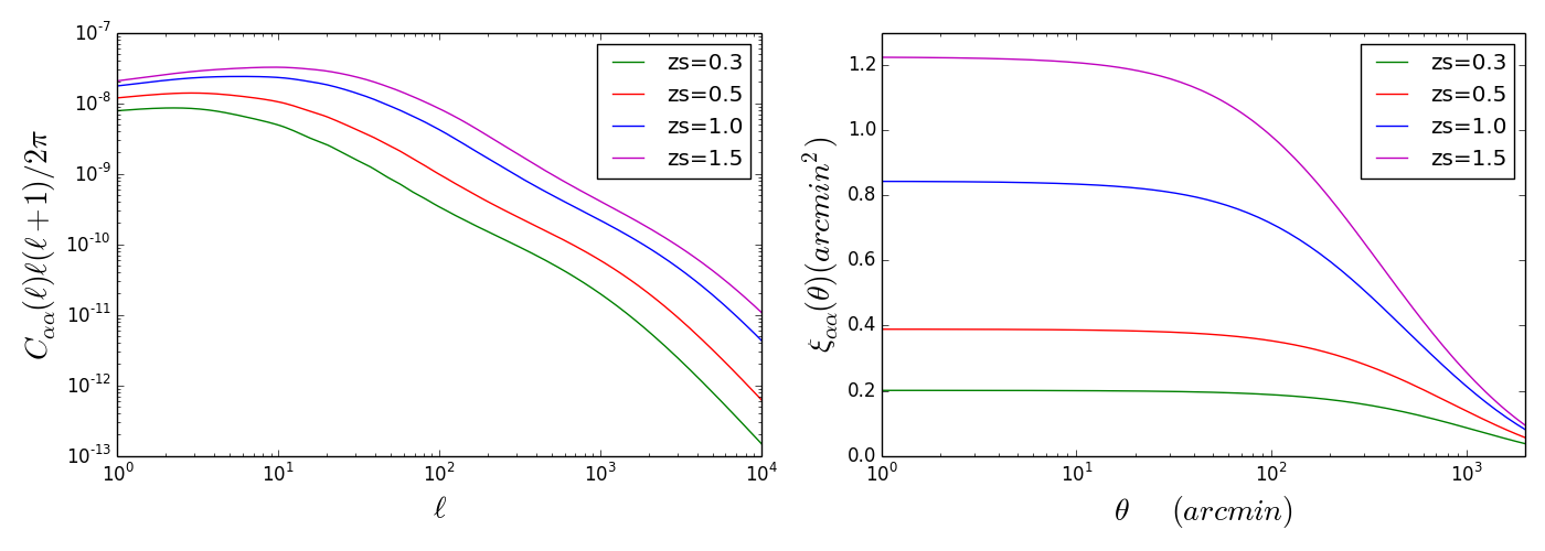
Figure 1: The power spectrum (left) and correlation function (right) for the deflection angle $\alpha$ due to weak lensing of sources at four different redshifts. The power peaks at $\ell<100$ for these redshifts, which corresponds to an angular scale above 1 degree. The correlation function is shown in units of arcmitute².

In the weak lensing regime, galaxy images are distorted. The distortion is effectively a mapping from the source plane to the image plane, which can be described by the lensing Jacobian $A$:

$$A=\begin{pmatrix}1-\kappa-\gamma_{1}&-\gamma_{2}\\ -\gamma_{2}&1-\kappa+\gamma_{1}\end{pmatrix},$$ (1)

where $\kappa$ is the convergence and $\gamma_{i}$ is the two-component shear. The convergence leads to a magnification of the object’s size and the shear causes an initially circular object to appear elliptical. The convergence $\kappa$ is a scalar quantity and is given by a weighted projection of the mass density fluctuation field:

$$\kappa(\mbox{{\it\boldmath$\theta$}})=\frac{1}{2}\nabla^{2}\Psi(\mbox{{\it\boldmath$\theta$}})=\int\!\!d\chi W(\chi)\delta[\chi,\chi\mbox{{\it\boldmath$\theta$}}].$$ (2)

We use the projected potential $\Psi$, with the Laplacian operator $\nabla^{2}$ defined using the flat sky approximation as $\nabla^{2}\equiv\partial^{2}/{\partial\mbox{{\it\boldmath$\theta$}}^{2}}$ and $\chi$ is the comoving distance (assuming a spatially flat universe). Note that $\chi$ is related to redshift $z$ via the relation $d\chi=dz/H(z)$, where $H(z)$ is the Hubble parameter at epoch $z$. The lensing efficiency function $W$ is given by

$$W(\chi)=\frac{3\Omega_{m0}H_{0}^{2}}{2c^{2}}\frac{\chi}{a(\chi)}\int\!\!d\chi_{s}~{}n_{s}(\chi_{s})\frac{\chi_{\rm s}-\chi}{\chi_{s}},$$ (3)

where $n_{s}(\chi_{s})$ is the redshift selection function of source galaxies, $H_{0}$ is the Hubble constant today, $\Omega_{m0}$ is the matter density today, and $c$ is the speed of light. For simplicity, we take source galaxies to be at a single redshift $z_{s}$, so that $n_{s}(\chi)=\delta_{D}(\chi-\chi_{s})$.

Here we are interested in the deflection angle, which at a given point in the photon trajectory is given by the transverse gradient of the gravitational potential: $-2\nabla_{\perp}\phi$. The projected lensing potential $\Psi$ above is defined by

$$\Psi=-2\int_{0}^{\chi_{s}}\frac{\chi(\chi_{s}-\chi)}{\chi_{s}}\phi(\chi)d\chi.$$ (4)

The net transverse deflection angle for a photon traveling from a source galaxy to the observer is then simply given by

$$\vec{\alpha}=\vec{\nabla}\Psi.$$ (5)

In Fourier space this gives

$$\tilde{\alpha}_{i}(\ell)=-\ell_{i}\tilde{\Psi}=\frac{2\ell_{i}\tilde{\kappa}(\ell)}{\ell^{2}}.$$ (6)

where $i=1,2$ corresponds to the x- and y-component of $\vec{\alpha}$. We can now write down the two-point correlation function of the deflection angles

$$\xi_{\alpha_{i}\alpha_{j}}(\theta)=\langle\alpha_{i}(\mbox{{\it\boldmath$\theta$}}_{1})\alpha_{j}(\mbox{{\it\boldmath$\theta$}}_{2})\rangle,$$ (7)

with $\theta=|\mbox{{\it\boldmath$\theta$}}_{1}-\mbox{{\it\boldmath$\theta$}}_{2}|$. We denote by $\xi_{\alpha\alpha}(\theta)$ the sum of the $x$- and $y$-components.

The deflection angle power spectrum at angular wavenumber $\ell$ is the Fourier transform of Equation 7. Using the equations above we can express it in terms of the mass density power spectrum $P_{\delta}$:

$$C_{\alpha\alpha}(\ell)=\frac{4C_{\kappa\kappa}(\ell)}{\ell^{2}}=\frac{4}{\ell^{2}}\int_{0}^{\chi_{s}}d\chi\,{W(\chi)^{2}\over\chi^{2}}P_{\delta}(\frac{\ell}{\chi},\chi).$$ (8)

The integral is dominated by the mass fluctuations at a distance about half-way to the source galaxies. The factor of $\ell^{2}$ in the denominator, compared to $C_{\kappa\kappa}$, leads displacements to be dominated by much larger scale modes than the convergence (or shear) fields.

Figure 1 shows the predicted power spectrum and angular correlation function of $\alpha$ assuming a standard dark energy dominated, spatially flat cosmology: $h=0.7$, $\Omega_{m}=0.3$, $w=-0.95$, $\sigma_{8}=0.8$, for four different source redshifts. Similar to $C_{\kappa\kappa}$, the amplitude is larger at high redshift, as there is more integrated matter causing the deflection. As noted above, the power spectrum for the deflection angles peaks at lower $\ell$. We discuss below the observational consequences of this feature.

3 Observational implication

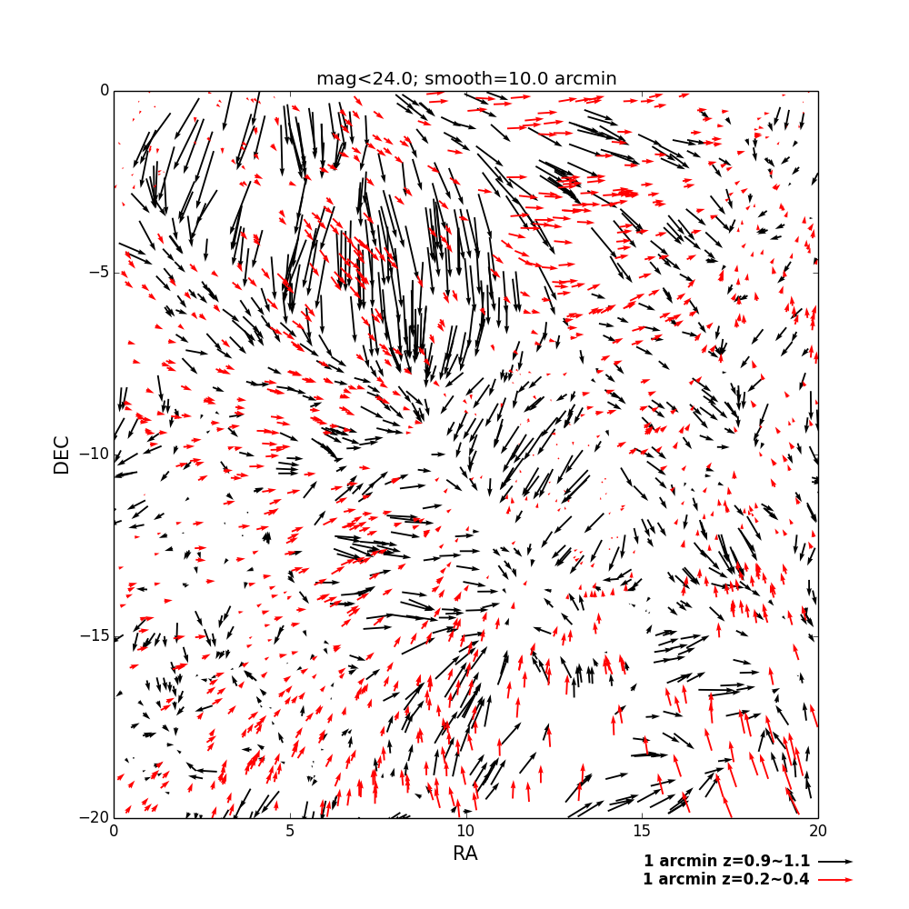
Figure 2: The displacement of galaxies is shown on a $20\times 20$ deg simulated patch. The arrows have a separate scale shown with the 1 arcmin arrow on the top right. They show the displacement due to lensing of source galaxies at two different redshifts: 0.3 in red and 1.0 in black. Note that the scale for the deflections is different from the scale on the x- and y-axis that shows the field of view. The displacements are fairly coherent on degree scales, but galaxies at different redshifts move relative to each other by up to an arcminute. So if we delens, say, a Hubble Deep Field sized patch of the sky, the galaxy locations will be scrambled!

We can now estimate the numerical values of the deflection angles and investigate implications. As discussed above, the peak of the power spectrum at $\ell<100$ means that the deflections are coherent over several degree-sized scales. Photons from source galaxies at redshift $\sim 1$, with co-moving distance of a few Gpc, are deflected by several tens of independent structures along their path to the observer. The physical picture is similar to a random walk – the further the source is, the more steps the photon will take in the random walk, therefore a larger deflection angle. The amplitude of the deflection, according to the correlation function in Figure 1, is of order 1 arcminute at redshift $\sim 1$. So galaxies at different redshifts are displaced by fractions of an arcminute, many times the typical separation of galaxies. This suggests that, if one were to effectively “delens” the galaxy positions on the sky, it will visibly shuffle the galaxies near each other on the sky but at different redshifts.

The lensing deflection and its redshift dependence can be visualised in simulations as shown in Figure 2. Details of the simulations are described in $\S$5.3. Figure 2 provides the visual picture of the deflection effect in observational data – galaxies at different redshifts are shuffled around at a significant level. Objects at high redshift ($z\sim 1$) are typically deflected more relative to the low-redshift ($z\sim 0.3$) objects, with the difference being of order an arcminute. The full field of the simulation is 20$\times$20 deg²; we can see that the deflections are coherent on degree-size patches.

The effect of this deflection field on a generic cosmological correlation function has been studied in Dodelson, Schmidt & Vallinotto (2008) and references therein. In particular, they pointed out that for galaxy correlation functions, the effect of the deflection field is generally at the percent level. Lensing deflections smooth out oscillating features in the correlation function (e. g. the BAO peak) just as they do for the CMB angular power spectrum.

In the next section we investigate the effect of the deflection field on one of the cosmological measurements that does not fall into the category of the general correlation functions studied in Dodelson, Schmidt & Vallinotto (2008). This measurement is especially relevant as it depends on correlating galaxies that are well separated in redshift – these galaxies are thus affected at a very different level by the deflection field as can be seen in Figure 2.

4 Galaxy-galaxy lensing

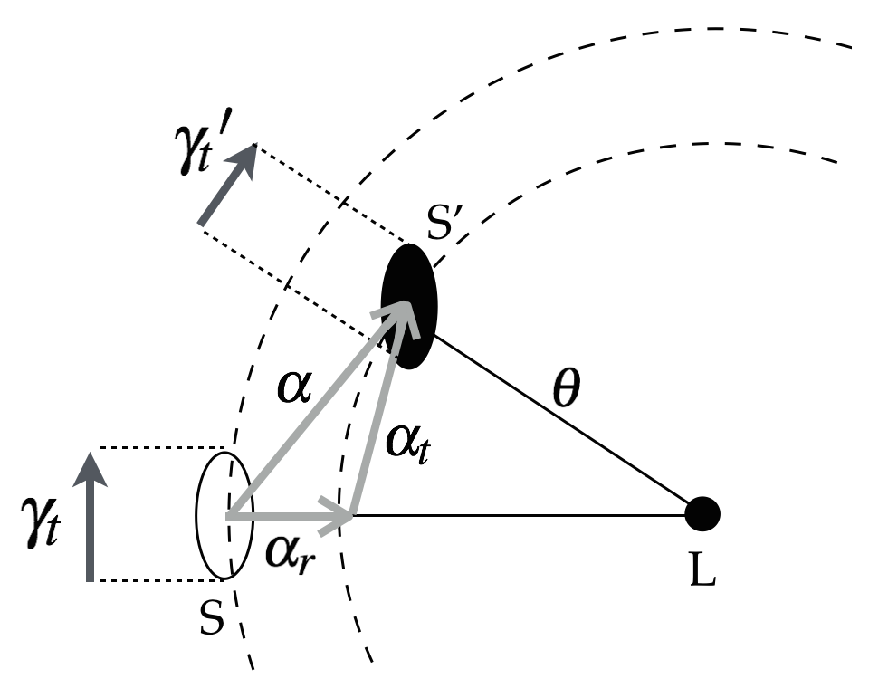
Figure 3: Illustration of the impact on galaxy-galaxy lensing from deflections between the lens and observer. The solid black ellipse (S’) represents the observed source galaxy whereas the hollowed ellipse (S) represents the true galaxy position. The solid circle (L) is the foreground lens galaxy. The deflection angle $\alpha$ can be decomposed into a radial ($\alpha_{r}$) and a tangential ($\alpha_{t}$) component with respect to the lens galaxy. $\alpha_{r}$ affects the relation between observed angular separation and transverse distance between source and lens: $\chi\theta\rightarrow\chi(\alpha_{r}+\theta)$. $\alpha_{t}$ affects the measured tangential shear signal. The true signal $\gamma_{t}$, indicated by the dark-grey arrow, is diluted to ${\gamma_{t}}^{\prime}$ because the apparent tangential direction has changed when the galaxy image is displaced.

Galaxy-galaxy lensing measures the cross-correlation of foreground galaxy positions with background galaxy shears. The cosmological signal can be measured by averaging the tangential component of the background galaxy ellipticities in circular annuli centered on the foreground galaxy, denoted as $\langle\gamma_{t}\rangle(\theta)$. $\langle\gamma_{t}\rangle(\theta)$ is directly translated into the projected mass density through $\Sigma(R)=\Sigma_{\rm crit}\gamma_{t}(\theta)$ (we drop the averaging notation here on). Deflections between the lens and observer can perturb the relative positions of the lens and source galaxy. In Figure 3 we illustrate both effects for one source-lens pair used to measure galaxy-galaxy lensing. The deflection angle $\vec{\alpha}$ is decomposed into a radial ($\alpha_{r}$) and a tangential component ($\alpha_{t}$). The figure shows how the two components introduce errors in the apparent source-lens distance and the measured tangential shear respectively.

For the radial deflection, we are interested in the mapping from measured angle to inferred spatial separation on the lens plane. We are interested in the rms quantity $\Delta\alpha_{r}(\theta)$, the uncertainty induced in the angular position of the source galaxy relative to the lens in the radial direction which smears out features in the $\langle\gamma_{t}\rangle(\theta)$ curve. It is given by:

$$\Delta\alpha_{r}(\theta)^{2}\equiv\frac{1}{2}\langle(\vec{\alpha}(0)-\vec{\alpha}(\theta))^{2}\rangle=\xi_{\alpha\alpha}(0)-\xi_{\alpha\alpha}(\theta).$$ (9)

The factor of 1/2 accounts for the fact that we are concerned with the radial component of $\Delta\vec{\alpha}$. $\Delta\alpha_{r}(\theta)$ has the effect of smearing the relation between observed angle $\theta$ and the distance from lens, i.e.

$$R=\chi\theta\rightarrow R=\chi(\theta\pm\Delta\alpha_{r}).$$ (10)

The mass profile $\Sigma(R)$ is then altered. We can estimate the effect by integrating over the foreground deflections, i.e. from $z=0$ to the lens redshift $z_{L}$. Figure 4 shows the calculated $\Delta\alpha_{r}(\theta)$ for lenses at redshift 0.5 and 1.0, along with the fractional error of the lens-source distance used in galaxy-galaxy lensing. At lens redshift $z_{L}=1$ and $\theta=10$ arcminutes, the error on the spatial separation between the source and the lens is about 1%. Depending on the shape of the $\langle\gamma_{t}\rangle(\theta)$ curve, this effect can introduce errors at different levels. It is only second order in $\Delta\alpha_{r}$, so unless the curvature is large, the effect is negligible. However, for particular cases such as satellite galaxy-galaxy lensing studied in Li et al. (2013), there can be sharp features in the curves, which would be smoothed out due to the deflection effect. Even for such cases we do not expect the effect to be a worry for ongoing surveys.

A second effect arises due to the deflection in the tangential direction: it lowers the estimated tangential shear $\langle\gamma_{t}\rangle(\theta)$ because the tangent direction itself is incorrect due to the deflections that occur between the source and the lens. Imagine a circle centered on the lens galaxy, the source galaxy position along that circle is changed by a differential deflection between lens and source. We choose the tangential direction based on its observed position, while the lens galaxy’s shear is tangent to the location where the light rays pass the lens plane. Unlike the radial effect, this does not depend on the shape of the $\langle\gamma_{t}\rangle(\theta)$ curve, but it is also a second order effect and is therefore well below a percent (note that the contribution to the “cross” component of the shear, usually used as a diagnostic of systematics, is first order and can be larger than a percent). Hence both effects may be relevant only for LSST and Euclid-era surveys that will achieve sub-percent statistical errors on the galaxy-galaxy lensing measurement.

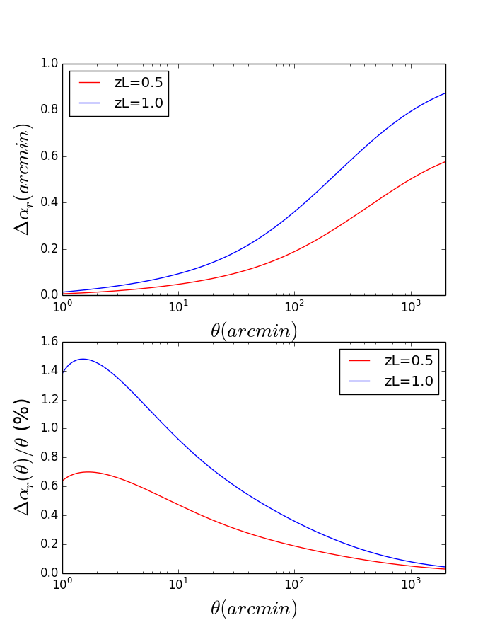
Figure 4: The radial component of the rms deflection angle $\Delta\alpha_{r}(\theta)$ vs. $\theta$ is shown in the top panel for two lens redshift $z_{L}=$0.5 and 1.0. The ratio $\Delta\alpha_{r}/\theta$ shown in the bottom panel is relevant for the observable effects discussed in the text.

5 Reconstruction of the deflection angle field

Consider now the possibility of reconstructing the galaxies’ true positions from observable quantities, which we will call “delensing”. We present two approaches to delensing that differ in how the convergence field $\kappa$ is obtained. The first method uses weak lensing shear measurements to construct the convergence field. The second uses the foreground galaxy density field with known galaxy bias to infer the convergence – this method is used if the shear-based convergence map is unavailable. The relation between the convergence and the lensing potential in Fourier space then follows from Equation 2 and Equation 5.

The fundamental limit of both methods is the finite size of the observed field. Since the reconstruction is a non-local operation, we cannot recover the full information with only limited Fourier modes inside the field. To first order, if we want to capture the dominant contributions to the deflection field, a field that spans linear scales $\sim$10 degrees ($\ell\sim 10$) or larger is required. As a result, shear-based reconstruction has only become feasible with ongoing lensing surveys such as DES. (The Canada-France Hawaii Telescope Lensing Survey covers $\sim 170$ deg² area, but the coverage is not contiguous.) Also note that operationally, constructing a continuous field from discrete galaxy measurements in both cases require smoothing and/or pixelization. As a result, there is also inevitable information loss on small scales, though this is not an issue in practice as we discuss below.

5.1 Reconstruction from weak lensing shear

The convergence can be calculated from the measured shear, which is a noisy but observable quantity. We use the method proposed by Kaiser & Squires (1993) to construct the continuous convergence map from shear. The Fourier transform of the observed shear relates to the convergence through

$$\kappa(\ell)-\kappa_{0}=D^{*}(\ell)\gamma(\ell),$$ (11)

where $\kappa_{0}$ is the average projected mass, i.e. $\kappa$ for $\ell=0$, and

$$D(\ell)=\frac{\ell_{1}^{2}-\ell_{2}^{2}+2i\ell_{1}\ell_{2}}{|\ell|^{2}}.$$ (12)

The major source of error in this approach comes from the large scatter in the galaxies’ intrinsic shape (shape noise), which contributes to a random error in the shear and therefore the $\kappa$ estimates. Since the deflection angle field is dominated by scales larger than a degree, the number density of galaxies is normally sufficient to ensure that shape noise smoothed on these scales is smaller than the signal. It is however not negligible for current surveys. Practically, the dominance of large angular scales also suggests that smoothing $\kappa$ to suppress the noise will not affect the inferred deflection angles.

5.2 Reconstruction from the galaxy density field

Alternatively, one can estimate the convergence field through the foreground galaxy density field if we assume some model for the galaxy bias $b$, so that $\delta_{g}=b\delta_{m}$, where $\delta_{g}$ is the over-density in the galaxy number counts and $\delta_{m}$ is the mass over-density. Note that in principle, $b$ could be a function of redshift and other galaxy properties. Using the linear bias relation, we can re-write the equation for $\kappa$, Equation 2, as:

$$\kappa(\mbox{{\it\boldmath$\theta$}})\approx\int\!\!d\chi W(\chi)b^{-1}\delta_{g}[\chi,\chi\mbox{{\it\boldmath$\theta$}}].$$ (13)

The main advantage of this approach in constructing $\kappa$ is that it by-passes the shape noise, and does not involve the Fourier transform in Equation 11 that introduces numerical errors in practice. An independent estimate of galaxy bias over the range of lens redshift, however, is needed for this method.

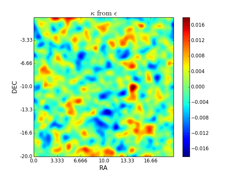
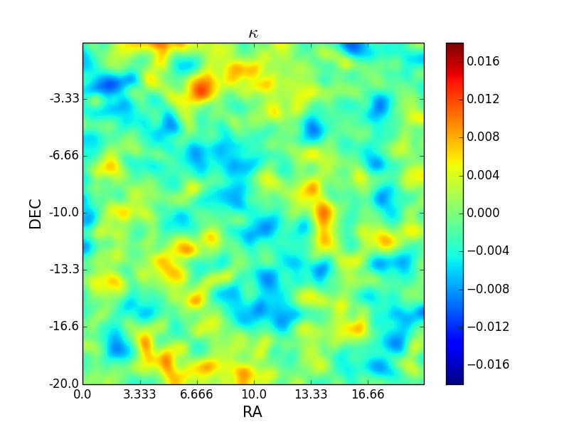
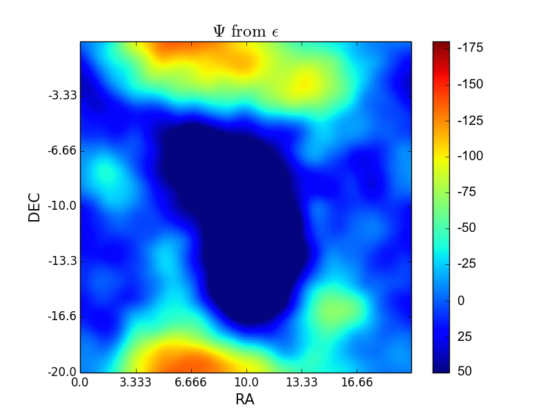
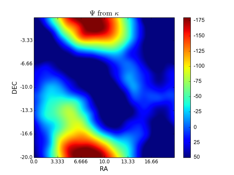
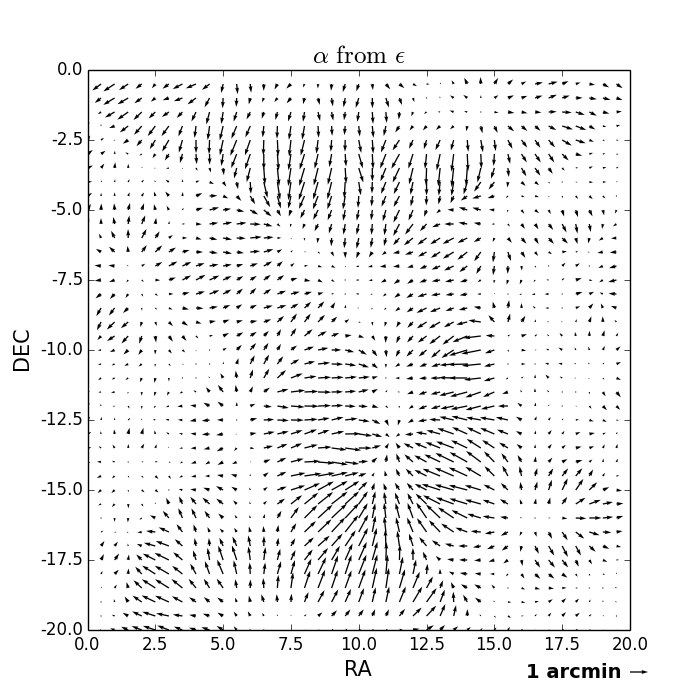
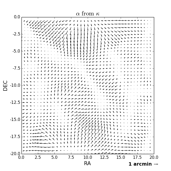
Figure 5: Maps generated for a 20$\times$20 deg² field, in the redshift range $0.9<z<1.1$. All maps are generated on 2$\times$2 arcminute² pixels with a 20 arcminute RMS Gaussian smoothing. Left: $\kappa$ (top), $\Psi$ (middle), and $\vec{\alpha}$ (bottom) maps generated from galaxy shape ($\epsilon$) measurements. These maps are generated with a galaxy sample with magnitude cut $i<24.0$, which is realistic for future wide-field surveys. Right: the same maps with the true $\kappa$. The difference between left and right shows the effect of shape noise as well as the $\kappa$ reconstruction from galaxy shapes.

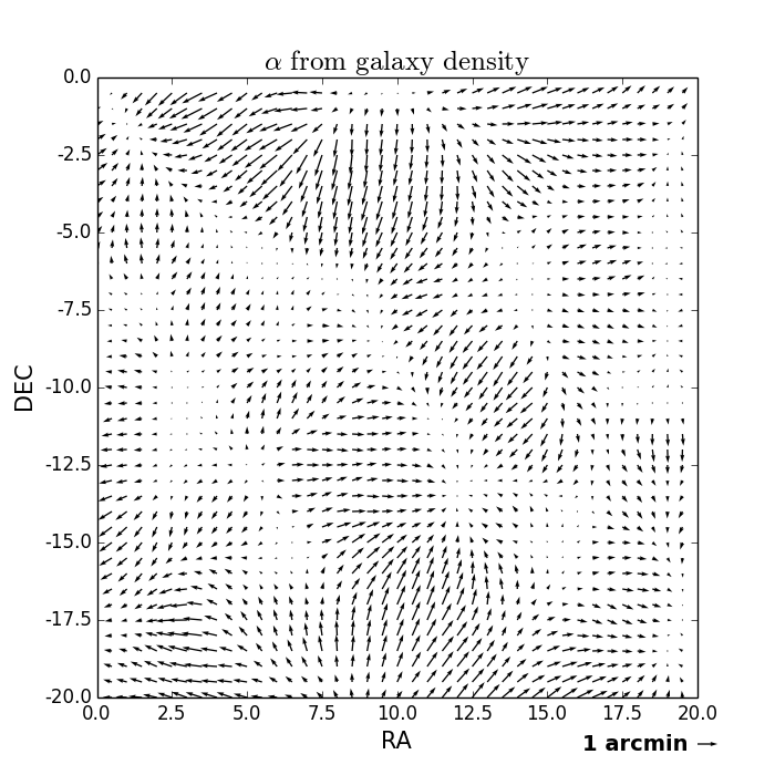
Figure 6: The $\kappa$ (left) and $\vec{\alpha}$ (right) field generated from the foreground galaxy density field, assuming a constant galaxy bias $b=2$. The reconstructed $\vec{\alpha}$ field is almost identical to that constructed from the true $\kappa$. This result depends on the simplicity and knowledge of galaxy bias.

5.3 Delensing simulations

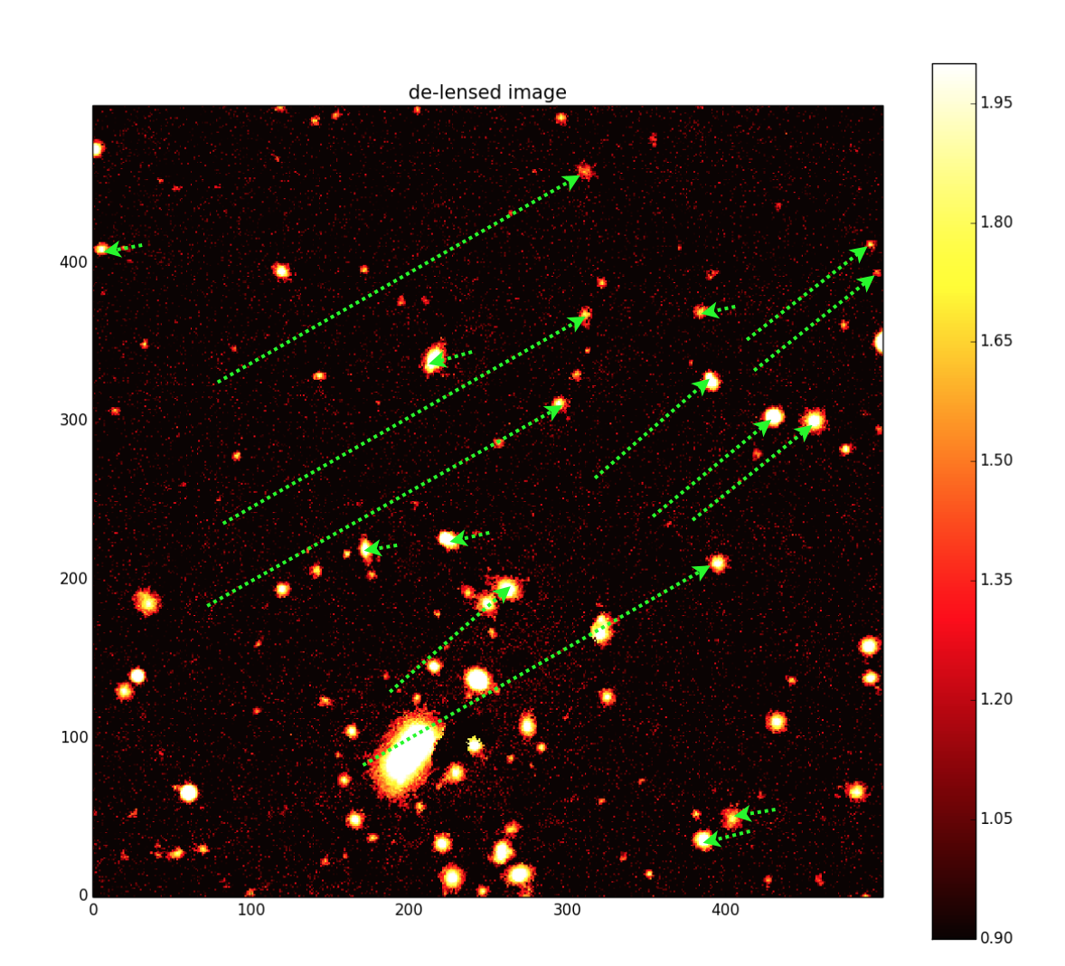
Figure 7: The delensed field (shown in detail below in Figure 8) with arrows indicating the displacement of some of the galaxies from the observed image to the de-lensed image. The galaxy position in the observed image is at the beginning of the arrow and it moves to the end-point of the arrow in the delensed image. The image size is 2.25$\times$2.25 arcminute² area. Visually one can see that there are three different lengths and orientations of the arrows in this image, associated with the three redshift bins shown in Figure 8. With tomographic lensing mass maps, displacement fields over a wide range of source redshifts can be obtained from wide field surveys.

A series of tests with simulations is shown here to demonstrate the operational steps in performing the reconstruction. We use the mock galaxy catalog generated by the algorithm Adding Density Determined Galaxies to Lightcone Simulations (ADDGALS; Wechsler et al, in preparation; Busha et al, in preparation). The lensing information (deflection angle, convergence and shear) is included for each galaxy according to a ray-tracing procedure described in Becker (2013). The total area of the full simulation covers a quarter of the sky. The lensing $\kappa$ maps are accurate down to about an arcminute, which is sufficient for our purposes. We use a 20$\times$20 deg² patch of the simulation to demonstrate the principle of reconstruction. The following parameters for each galaxy in the catalog are used: true position, lensed position, magnitude, ellipticity $\epsilon$, convergence $\kappa$, and shear $\gamma$ at the lensed position. Previously we have shown in Figure 2 an example of the deflection angles of galaxies for two different redshifts from the simulations.

We first demonstrate the reconstruction procedure described in $\S$5.1. We use the high-redshift galaxy sample (0.9$<$z$<$1.1) in Figure 2 with a magnitude cut of $i<24$ to simulate what is expected in a magnitude-limited dataset. In the 20$\times$20 deg² area, there are $\sim$2.68/arcmin² galaxies in this sample. The median redshift is $\sim 1.0$. We pixelate the $\epsilon$ values into a 600$\times$600 grid, with each pixel being 2$\times$2 arcmin². The rms of the ellipticity distribution per component (i.e. shape noise per shear component) is $\sim 0.27$ at this magnitude cut. We then apply a 20 arcminute rms Gaussian smoothing to the maps to suppress noise (Kaiser & Squires, 1993). The $\epsilon$ maps are converted to $\kappa$ maps according to Equation 11. From the $\kappa$ maps we reconstruct the lensing potential $\Psi$ according to Equation 2. And finally we calculate the $\vec{\alpha}$ field using Equation 6. The left panel of Figure 5 shows the series of maps generated in this procedure. The right panel of Figure 5 shows the same series of maps but using the true $\kappa$ instead of using $\epsilon$ to make the $\kappa$ maps. The difference in the two panels comes from shape noise as well as errors introduced in Equation 11. The median error in the reconstructed $\vec{\alpha}$ compared to the true $\vec{\alpha}$ in the simulations is $\sim 30$ degrees in the direction angle of and $50\%$ in the magnitude of $\vec{\alpha}$. The reconstruction degrades when reducing the area of the simulation used. With a factor of $\sim$8 smaller area, the reconstruction is essentially consistent with noise. This confirms that most of the power in the deflection field comes from the large scales. Several other sources of intrinsic errors are expected in this reconstruction:

• We have implicitly assumed the average $\kappa$ is approximately the same as the $\kappa$ at the median redshift of the sample.

• The galaxy intrinsic shape introduces noise in the $\kappa$ maps and therefore the reconstruction.

• Numerical errors in the simulation, interpolation and the flat sky approximation – these are expected to be negligible.

Next, we demonstrate the reconstruction procedure based on the foreground galaxy distribution, described in $\S$5.2. We construct the $\kappa$ map using galaxies from $z=0$ to $z=1$, weighted by the lensing kernel $W(\chi)$ (Equation 3). We assume a constant bias $b=2.0$ and a magnitude cut of $i<24$. The $\Psi$ and $\vec{\alpha}$ maps are then obtained as before. The $\kappa$ and the final $\vec{\alpha}$ maps from this approach are shown in Figure 6. We find that the $\vec{\alpha}$ map reconstructed in this fashion is much less noisy given that there is no scatter from associated with shape noise. The rms error between the $\kappa$ map generated from the ellipticities and the true $\kappa$ map in our test is $\sim$0.0036, whereas the rms error for the $\kappa$ map generated from the galaxy density is $\sim 0.0009$. However, the method requires a priori knowledge of galaxy bias before performing the reconstruction. The fact that we get good results is likely due to the simplicity of the galaxy assignment in the simulations.

One possible improvement to the two reconstruction methods discussed above is to combine the two, similar to Amara et al. (2012) and use the information in the density field as well as the shear field to constrain the deflection and the bias simultaneously. Note that we only need an estimate of the average bias on large scales over the lens redshift range, thus the bias is needed to less accuracy compared to that used in Amara et al. (2012).

6 Conclusion

We have studied lensing deflections in the context of ongoing and planned wide-field galaxy surveys. The power spectrum of the deflection field peaks at large angular scales, so the deflections are coherent over degree-sized scales. The rms deflection is about one arcminute at redshift $\sim 1$. The redshift-dependence of the deflection field implies that galaxies that are nearby on the sky can be displaced by fractions of an arcminute relative to each other. So measurements requiring cross-correlation of galaxies at different redshift can be affected. We discuss galaxy-galaxy lensing and estimate that the error associated with ignoring the deflection field is at the sub-percent level and therefore not a concern for ongoing lensing surveys. It may be worth examining further for particular galaxy lens populations for LSST and Euclid-era surveys.

The main purpose of the paper is to undo the effect of deflections on wide field images by “delensing” galaxy positions. We implement two approaches to delensing: one is based on mass maps that use the measured lensing shear, while the second uses the galaxy density field as a proxy for the lensing mass distribution. We show that a field of several hundred square degrees is required for the reconstruction to be reasonably accurate. We expect better reconstructions with even larger fields. Ongoing imaging surveys such as DES will for the first time have the capability to delens the galaxy distribution.

Once the deflection field is reconstructed, one can delens the pixel-level images via standard image-remapping programs (e.g. OpenCV). In Figure 7 we demonstrate an example of delensing the simulated sky by remapping every pixel in the image. We bin the galaxies into 4 redshift bins, and delens each bin by the deflection field at the mean redshift of that bin. Noise and stars are not delensed. For visualization purposes, we zoom into a 2.25$\times$2.25 arcminute² area (500$\times$500 pixels in our simulated image). We can see a clear change in the galaxy apparent positions on the sky. More details of the image generation are described in Appendix A. Tomographic lensing mass maps from wide field surveys will allow us to reconstruct the entire trajectories of lights rays from distant galaxies to us.

Appendix A Pixel-level delensing

We perform a pixel-level delensing using images simulated by the Ultra Fast Image Generator (Bergé et al., 2013). Pixels associated with each object are identified with the software Source Extractor (Bertin & Arnouts, 1996), then remapped according to the displacement field at that redshift using the OpenCV software. There are visible image artefacts associated with the fact that we can only delens on individual pixels in this approach, i.e. thus blended objects cannot be individually delensed. The upper panel of Figure 8 shows the original image as in Figure 7 and the lower panels show how we decompose the image into the different redshift components.

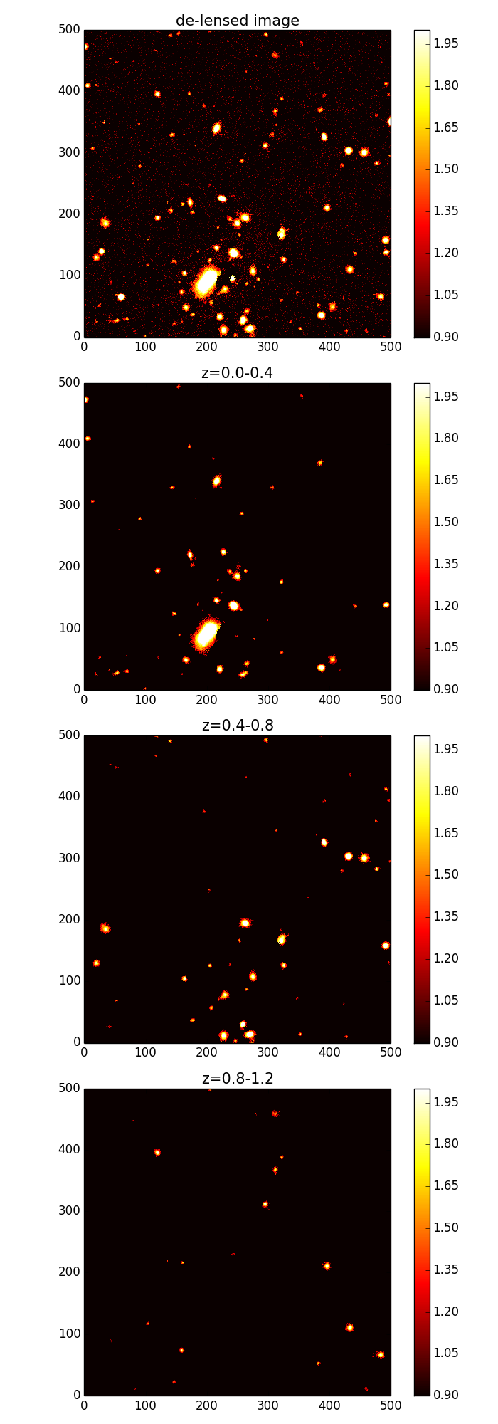
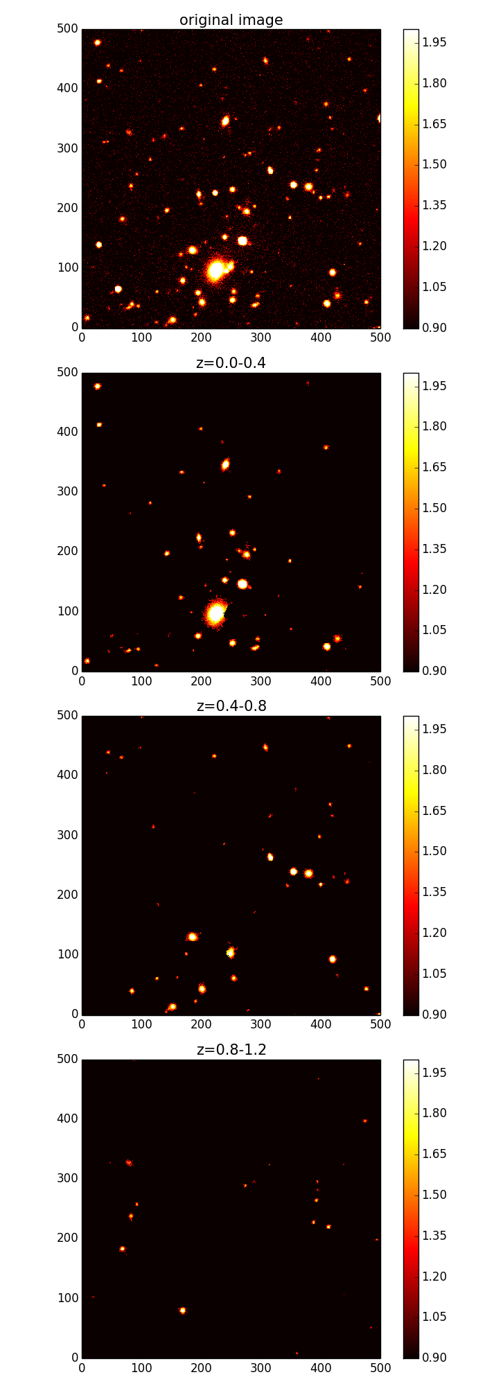
Figure 8: An example of pixel-level delensing with simulations. The observed images on the left is delensed into the right-hand-side images. The top panel is the full image (same as Figure 7), which is a sum of the different redshift components. We show three redshift bins in the bottom three rows, which correspond to the three coherent fields in Figure 7 that have different lengths of arrows. Visually we can see the high-redshift bins are shifted the most, and the relative relation between objects are changed significantly before and after lensing. Note also that the $0.0<z<0.4$ bin shifts in an opposite direction compared to the others. All images are 500$\times$500 pixels, with pixel scale is 0.27”, which yields a 2.25$\times$2.25 arcminute² area. The image colours are in logarithmic scales.

Acknowledgement. We acknowledge helpful discussions with Adam Amara, Gary Bernstein, Sarah Bridle, Joseph Clampitt, Eric Huff, Elisabeth Krause and Mike Jarvis. We are grateful to Vinu Vikram for discussions and related collaborative work. We thank the simulation team, especially Matt Becker, Michael Busha and Risa Wechsler, responsible for the mock catalogs used in our tests and Lukas Gamper and Joel Berge for the image simulations. This work is supported in part by the Department of Energy grant DE-SC0007901 and the Swiss National Science Foundation grant 200021-149442.

References

- Amara et al. (2012) Amara A. et al., 2012, MNRAS, 424, 553
- Bartelmann & Schneider (2001) Bartelmann M., Schneider P., 2001, Physics Reports, 340, 291
- Becker (2013) Becker M. R., 2013, MNRAS, 435, 115
- Bergé et al. (2013) Bergé J., Gamper L., Réfrégier A., Amara A., 2013, Astronomy and Computing, 1, 23
- Bertin & Arnouts (1996) Bertin E., Arnouts S., 1996, A&AS, 117, 393
- Dodelson, Schmidt & Vallinotto (2008) Dodelson S., Schmidt F., Vallinotto A., 2008, Phys.Rev.D, 78, 043508
- Heymans et al. (2012) Heymans C. et al., 2012, MNRAS, 427, 146
- Hoekstra & Jain (2008) Hoekstra H., Jain B., 2008, Annual Review of Nuclear and Particle Science, 58, 99
- Huff & Graves (2011) Huff E. M., Graves G. J., 2011, ArXiv e-prints: arXiv/1111.1070
- Jee et al. (2013) Jee M. J., Tyson J. A., Schneider M. D., Wittman D., Schmidt S., Hilbert S., 2013, ApJ, 765, 74
- Kaiser (1998) Kaiser N., 1998, ApJ, 498, 26
- Kaiser & Squires (1993) Kaiser N., Squires G., 1993, ApJ, 404, 441
- Lewis & Challinor (2006) Lewis A., Challinor A., 2006, Physics Reports, 429, 1
- Li et al. (2013) Li R., Mo H. J., Fan Z., Yang X., Bosch F. C. v. d., 2013, MNRAS, 430, 3359
- Refregier (2003) Refregier A., 2003, ARA&A, 41, 645
- Vallinotto et al. (2007) Vallinotto A., Dodelson S., Schimd C., Uzan J.-P., 2007, Phys.Rev.D, 75, 103509