The role of numerical boundary procedures in the stability of perfectly matched layers

Abstract

In this paper we address the temporal energy growth associated with numerical approximations of the perfectly matched layer (PML) for Maxwell’s equations in first order form. In the literature, several studies have shown that a numerical method which is stable in the absence of the PML can become unstable when the PML is introduced. We demonstrate in this paper that this instability can be directly related to numerical treatment of boundary conditions in the PML. First, at the continuous level, we establish the stability of the constant coefficient initial boundary value problem for the PML. To enable the construction of stable numerical boundary procedures, we derive energy estimates for the variable coefficient PML. Second, we develop a high order accurate and stable numerical approximation for the PML using summation–by–parts finite difference operators to approximate spatial derivatives and weak enforcement of boundary conditions using penalties. By constructing analogous discrete energy estimates we show discrete stability and convergence of the numerical method. Numerical experiments verify the theoretical results.

1 Introduction

Numerical approximations of the perfectly matched layer (PML) [1, 14] for Maxwell’s equations in first order form often exhibit a late time linear or exponential energy growth, see for example [3, 2, 12, 11]. This unwanted growth can spread into the computational domain and ruin the accuracy of a numerical simulation. Growth is often seen long after a wave has exited the domain or when a wave has been trapped in the domain for a longtime. The later situation can occur, for example, in the simulation of an electromagnetic waveguide. This has generated substantial interests. One explanation for this behavior of the PML was offered in [4]. It is shown that the split–field PML is weakly hyperbolic, and numerical approximations can lead to perturbations that excite explosive modes in the PML. Because of the result in [4], several unsplit (strongly hyperbolic) PMLs for Maxwell’s equations were developed [1]. However, series of numerical experiments presented in the literature, see for instance [3, 2], using standard finite difference schemes and [7] for finite element methods, suggest that these unsplit PMLs also suffer from the same late time exponential energy growth as the split field PML. It was later shown in [3] that the source of the late time exponential growth was characterized by the multiplicity of eigenvalues and the degeneracy of eigenvectors of the lower order undifferentiated terms. In [11, 12], however, it was shown, for a given computational setup, that the growth generated in the PML, if any, may not propagate back into the computational domain. It is also important to note that a partial remedy for this problem in odd (1 and 3) spatial dimensions has been proposed in [46], using a lacunae based time integration. Nonetheless, a recent analysis of a PML for Maxwell’s equations in [21] shows that the corresponding initial value problem (IVP) is asymptotically stable. In this study, we argue that many of the late time energy growth of the PML for Maxwell’s equations observed in computations are caused by inadequate numerical boundary treatments in the PML.

We denote that the well–posedness and temporal stability analysis of the PML has been a topic of several works, see for instance [10, 41, 32, 7, 4, 3, 2, 1, 46, 36, 22, 21, 20, 12, 11, 9] and many others. In [32], perfect matching, well-posedness and temporal stability for PMLs as well as some other classes of layers are discussed for general systems. Unfortunately, there is no guarantee that all solutions decay with time. In [10] however, the geometric stability condition was introduce to characterize the temporal stability of IVP for the PML. If this condition is not satisfied, then there are modes of high spatial frequencies with temporally growing amplitudes. In this paper, we consider a two space dimensional model problem satisfying the geometric stability condition but augmented with boundary conditions in the tangential and normal directions. Our primary objective in this paper is the analysis and development of high order accurate and provably stable numerical approximations of the corresponding initial boundary value problem (IBVP).

It is a well known fact that the theory and numerical techniques to solve an IBVP are more elaborate and complicated than that of a corresponding IVP. For a well–posed partial differential equation which is stable in the absence of boundaries can support unstable solutions, or become ill–posed, when boundaries are introduced. In fact, the analysis of the IVP is a necessary (first) step towards the analysis of the IBVP [38, 39, 44]. For symmetric hyperbolic systems such as the Maxwell’s equations and certain boundary conditions, using the energy method, it is possible to obtain a uniform bound on the L₂–norm of the solutions (electric and magnetic fields) in terms of the L₂–norm of the initial data and a boundary norm of the boundary data [30, 29, 28]. In numerical approximations of IBVPs, most of the difficulties arise from the boundaries. Similarly, a numerical method which is stable in the absence of boundaries can support growth when boundary conditions are imposed. In the discrete setting, it is possible though to design stable numerical boundary procedures by mimicking the continuous estimates [5, 6, 45, 26, 27, 43].

Effective boundary treatments are also important when PMLs are used in computations. If there are physical boundaries, for instance in waveguides [20, 19], the corresponding boundary conditions must be accurately extended into the PML. In practice, the PML must be solved on a bounded computational domain. A stable and accurate PML boundary closure becomes essential, since it enables efficient numerical computations. There is an ongoing discussion though on how to effectively terminate the PML. It is also important to point out that a numerical method which is stable in the absence of the PML can support growth when the PML is included. A major difficulty is that in general the PML (for symmetric systems) is asymmetric. Therefore, deriving energy estimates for the PML that are useful in designing stable and accurate numerical boundary procedures can be very challenging. Linear and/or exponential temporal growth are frequently seen in numerical simulations of PMLs [3, 2, 46], particularly if higher order methods are considered. Often, artificial numerical dissipations are added to the scheme in order to eliminate these unwanted temporal growth. Artificial numerical dissipations certainly helps in many ways, but can also introduce some interesting, and unfortunately undesirable, effects. In standard computational electromagnetic codes, discrete stability of the numerical method is usually investigated in the absence of the PML. Once the interior scheme is confirmed stable, the PML is then included by discretizing the accompanying auxiliary differential equations and appending the auxiliary functions accordingly, without further discrete stability analysis. As in [3, 2, 46], any eventual growth seen when the absorption function is present is then attributed to the PML. We emphasize that a more complete analysis of discrete stability must include all the equations and variables in the PML.

In bounded and semi–bounded domains the stability of the PML has been analyzed for certain classes of problems and boundary conditions [19, 18] using normal mode analysis. These results [19, 18] are mostly for second order systems. In the continuous setting, it is possible to extend some of these theoretical results to the PML for first order systems. However, numerical treatments for first order systems are essentially different from numerical methods for second order systems. For instance, standard boundary conditions for first order hyperbolic systems can only contain a linear combination of the unknown variables, while boundary conditions for second order systems often involve combinations of the unknown variables and their spatial and temporal derivatives. Therefore, for first order systems different numerical techniques and, probably, new theories are required.

In the present paper, we consider unsplit PMLs [3, 2, 21] and the classical split–field PML [14] , for Maxwell’s equations in first order form with boundary conditions set by an electromagnetic waveguide. We are particularly interested in high order accurate and efficient methods for numerical simulation of Maxwell’s equations. Our first objective is to extend the continuous analysis for Cauchy problems [21] to the PML in semi–bounded and bounded domains. The first sets of results are the proofs of stability of the constant coefficient PML in a lower half–plane and a left half–plane. The second results in the paper are the derivation of energy estimates for constant coefficients in the Laplace space and for variable coefficients PML in the time domain.

We show that a stable numerical boundary procedure for the undamped problem can become unstable when the PML is introduced.

The second objective of the paper is to develop a high order accurate and provably stable numerical approximation for the PML in a bounded domain. We use summation–by–parts (SBP) finite difference operators [26, 48] to approximate spatial derivatives. Boundary conditions are enforced weakly using a penalty technique, referred to as the simultaneous approximation term (SAT) methodology [15, 43, 45]. By mimicking the continuous energy estimates we construct accurate and stable boundary procedures. The convergence of the numerical method follows. Finally, we present numerical experiments, using SBP finite difference operators in space with interior order of accuracy 2, 4 and 6, and the classical fourth order accurate Runge–Kutta scheme in time. The numerical examples illustrate high order accuracy and longtime stability of the PML.

Note that in [3, 2] it was pointed out that the discrete PML for Maxwell’s equations in first order form can suffer severely from longtime exponential energy growth when spatial derivatives are discretized with high order accurate central finite difference operators and and the time derivative discretized using Runge–Kutta schemes. This indicates that an appropriate remedy is required. The results obtained in this paper provide a cure for this problem without any additional cost. We believe that the results obtained in this paper can be extended to other situations, not only for finite difference electromagnetic codes, but also for finite volume methods, finite element methods and spectral methods, and for more complicated systems such as the elastic wave equation in isotropic media and the linearized Euler equation with vanishing mean flow.

The remainder of the paper is planned as follows. In the next section, we present some preliminaries, introducing Maxwell’s equations in two space dimensions and a brief description of a discrete approximation of the Maxwell’s equations in a bounded domain using the SBP-SAT methodology. In section 3, we introduce the PMLs and present some instructive numerical experiments, motivating the continuous analysis in section 4 and the discrete analysis in section 5. In section 5, we construct discrete approximations for the PML, derive discrete energy estimates and prove asymptotic stability. More numerical experiments are presented in section 6, verifying the analysis of previous sections. A summary of the paper and suggestions for future work are offered in the last section.

2 Preliminary

Here, we introduce the Maxwell’s equations in a two dimensional rectangular domain. We end the section with a brief description of the SBP–SAT methodology for Maxwell’s equations.

2.1 The Maxwell’s equations in a rectangular domain

Consider the transverse magnetic $(TM_{z})$ case of the Maxwell equation in a source free, homogeneous isotropic medium,

$$\begin{split}&\frac{\partial{E_{z}}}{\partial t}=-\frac{\partial{H_{y}}}{\partial x}+\frac{\partial{H_{x}}}{\partial y},\\ &\frac{\partial{H_{y}}}{\partial t}=-\frac{\partial{E_{z}}}{\partial x},\\ &\frac{\partial{H_{x}}}{\partial t}=\frac{\partial{E_{z}}}{\partial y}.\\ \end{split}$$ (1)

Here, $\textbf{H}=\left(H_{x},H_{y},0\right)^{T},\quad\textbf{E}=\left(0,0,E_{z}\right)^{T}$ are the magnetic fields and electric fields respectively. At the initial time $t=0$ we set the smooth initial data

$$\left(E_{z}\left(x,y,0\right),H_{y}\left(x,y,0\right),H_{x}\left(x,y,0\right)\right)^{T}=\left(f_{1}(x,y),f_{2}(x,y),f_{3}(x,y)\right)^{T}.$$

Consider now the two space dimensional rectangular domain $\left(x,y\right)\in[-x_{0}-\delta,x_{0}+\delta]\times[-y_{0},y_{0}]$, with $x_{0},y_{0},\delta>~{}0$. The length and width of the rectangle are $\Gamma_{x}:=\{x:-x_{0}-\delta\leq x\leq x_{0}+\delta\}$ and $\Gamma_{y}:=\{y:-y_{0}\leq y\leq y_{0}\}$. At the edges of the rectangle, at $x=\pm\left(x_{0}+\delta\right)$ and $y=\pm y_{0}$, we set the general boundary conditions, expressed as a relation between the incoming and outgoing characteristics

$$\frac{1}{2}\left({E_{z}\mp H_{y}}\right)=\frac{R_{x}}{2}\left(E_{z}\pm H_{y}\right)\iff\frac{\left(1-R_{x}\right)}{2}E_{z}\mp\frac{\left(1+R_{x}\right)}{2}H_{y}=0,\quad\text{at}\quad x=\pm\left(x_{0}+\delta\right),$$ (2)

$$\frac{1}{2}\left(E_{z}\pm H_{x}\right)=\frac{R_{y}}{2}\left(E_{z}\mp H_{x}\right)\iff\frac{\left(1-R_{y}\right)}{2}E_{z}\pm\frac{\left(1+R_{y}\right)}{2}H_{x}=0,\quad\text{at}\quad y=\pm y_{0}.$$ (3)

Here, the reflection coefficients $R_{j}$ $(j=x,y),$ with $|R_{j}|\leq 1$, are real constants. Note that the boundary condition (2), (3) can support boundary waves: waves whose amplitudes are maximum on the boundaries, at $x=\pm\left(x_{0}+\delta\right)$, $y=\pm y_{0}$, but decay exponentially into the domain. In particular if $R_{j}=1$, then the boundary conditions (2), (3) model insulated electromagnetic walls. Glancing waves, constant modes normal to the boundaries, can be supported. If $R_{j}=-1$, then the boundary conditions (2), (3) model perfect electric conductor (PEC) boundary conditions. And if $R_{j}=0$, then the boundary conditions (2), (3) correspond to local one dimensional absorbing boundary conditions, which are also equivalent to setting the incoming characteristics (Riemann invariant) at the boundaries to zero.

Note that if $R_{j}\neq-1$ then we have

$$\gamma_{x}E_{z}\mp H_{y}=0,\quad\text{at}\quad x=\pm\left(x_{0}+\delta\right),\quad\gamma_{x}=\frac{\left(1-R_{x}\right)}{\left(1+R_{x}\right)}\geq 0,$$ (4)

$$\gamma_{y}E_{z}\pm H_{x}=0,\quad\text{at}\quad y=\pm y_{0},\quad\gamma_{y}=\frac{\left(1-R_{y}\right)}{\left(1+R_{y}\right)}\geq 0.$$ (5)

The special case of $R_{j}=-1$ in (2), (3) corresponds to PEC boundary conditions

$$E_{z}=0,\quad\text{at}\quad x=\pm\left(x_{0}+\delta\right),$$ (6)

$$E_{z}=0,\quad\text{at}\quad y=\pm y_{0}.$$ (7)

Let the standard $L_{2}$ inner product and the corresponding norm be defined by

$$\left(u,v\right)=\int_{\Omega}v^{*}u\mathrm{d}x\mathrm{d}y,\quad\|u\|^{2}=\left(u,u\right).$$ (8)

We also introduce the boundary norms $\|\cdot\|^{2}_{\Gamma_{x}}$, $\|\cdot\|^{2}_{\Gamma_{y}}$, defined by

$$\left(u_{0},v_{0}\right)_{\Gamma_{z}}=\int_{\Gamma_{z}}v_{0}^{*}u_{0}\mathrm{d}z,\quad\|u_{0}\|^{2}_{\Gamma_{z}}=\left(u_{0},u_{0}\right)_{\Gamma_{z}},\quad z\in\Gamma_{z},\quad z=x,y.$$ (9)

Here, $v^{*},v_{0}^{*}$ are the complex conjugates of $v,v_{0}$ and $u_{0}(z),v_{0}(z)$ depend on one spatial variable $z=x$ or $z=y$. Using the energy method and integration by parts, it is straightforward to show that the Maxwell’s equation (1) subject to the boundary conditions (4), (5), with $\gamma_{j}\geq 0$, satisfies

$$\begin{split}&\|E_{z}\left(t\right)\|^{2}+\|H_{y}\left(t\right)\|^{2}+\|H_{x}\left(t\right)\|^{2}+2\gamma_{x}\int_{0}^{t}\left(\|E_{z}\left(t^{\prime},x_{0}+\delta\right)\|^{2}_{\Gamma_{y}}+\|E_{z}\left(t^{\prime},-x_{0}-\delta\right)\|^{2}_{\Gamma_{y}}\right)dt^{\prime}\\ &+2\gamma_{y}\int_{0}^{t}\left(\|E_{z}\left(t^{\prime},y_{0}\right)\|^{2}_{\Gamma_{x}}+\|E_{z}\left(t^{\prime},-y_{0}\right)\|^{2}_{\Gamma_{x}}\right)dt^{\prime}=\|f_{1}\|^{2}+\|f_{2}\|^{2}+\|f_{3}\|^{2}.\end{split}$$ (10)

In particular if $\gamma_{j}=0$ in (4), (5) or $R_{j}=-1$ (we consider the PEC condition) in (2), (3) then

$$\|E_{z}\left(t\right)\|^{2}+\|H_{y}\left(t\right)\|^{2}+\|H_{x}\left(t\right)\|^{2}=\|f_{1}\|^{2}+\|f_{2}\|^{2}+\|f_{3}\|^{2}.$$ (11)

Note that the $L_{2}$-norm of the solutions (electric and magnetic fields) are uniformly bounded in time by the $L_{2}$-norm of the initial data.

2.2 A stable discrete approximation of the Maxwell’s equations using the SBP–SAT methodology

This subsection serves as a brief introduction to the SBP–SAT scheme for IBVPs (Maxwell’s equations in bounded domains). The main idea is to approximate all spatial derivatives in (1) using SBP finite difference operators. The boundary conditions (4), (5) are then enforced weakly using penalties. However, penalty parameters must be chosen such that discrete energy estimates, analogous to the continuous estimates (10), (11), can be derived. Thus, proving asymptotic stability for the discretization. More elaborate discussions on this topic can be found in [5, 6, 26, 27, 15, 43, 45], see also the recent review paper [49].

To begin with, consider the uniform discretization of the unit interval with $N_{x}$ number of grid points and the spatial step, $h>0$,

$$x_{i}=\left(i-1\right)h,\quad i=1,2,\dots,N_{x},\quad h=\frac{1}{N_{x}-1}.$$ (12)

Let $D_{x}$ denote a differentiation matrix approximating the first derivative, $D_{x}\approx{\partial}/{\partial x},$ on the grid (12). The matrix $D_{x}$ is an SBP operator (in one space dimension), see [26, 48], if the following properties hold

$$\begin{split}&D_{x}=\mathrm{P}_{x}^{-1}Q_{x},\quad Q_{x}^{T}+Q_{x}=E_{Rx}-E_{Lx}.\end{split}$$ (13)

Here, $E_{Lx}=\mathrm{diag}(1,0,0,\ldots,0)$, $E_{Rx}=\mathrm{diag}(0,0,0,\ldots,1)$ pick out the left and right boundary values. The matrix $\mathrm{P}_{x}$ is symmetric and positive definite, and thus defines a discrete norm. The matrix $Q_{x}$ is almost skew-symmetric.

It is important to note that SBP operators can be constructed using Galerkin finite/spectral element approaches [24, 35]. The one space dimensional SBP operator $D_{x}$ can be extended to higher space dimensions using the Kronecker product, $\otimes$, defined by

Definition 1 (Kronecker Products).

Let A be an m-by-n matrix and B be a p-by-q matrix. Then $A\otimes B$, the Kronecker product of A and B, is the (mp)-by-(nq) matrix

$$A\otimes B=\begin{pmatrix}a_{11}B&a_{12}B&\ldots&a_{1n}B\\ [4]{4}\\ [4]{4}\\ a_{m1}B&a_{m2}B&\ldots&a_{mn}B\end{pmatrix}.$$

The following properties hold for Kronecker products

1. Assume that the products AC and BD are well defined then
   $(A\otimes B)(C\otimes D)=(AC)\otimes(BD)$,

2. If A and B are invertible, then $(A\otimes B)^{-1}=A^{-1}\otimes B^{-1}$,

3. $(A\otimes B)^{T}=A^{T}\otimes B^{T}$.

Now consider the Maxwell’s equation in a two dimensional rectangular domain. To begin, we discretize the spatial domain in the $x$- and $y$-directions using $N_{x},N_{y}$ grid points with constant spatial steps $h_{x},h_{y}$, respectively. A two dimensional scalar grid function, $\mathbf{u}=[u_{ij}]$, is stacked as a vector of length $N_{x}N_{y}$,

$$\mathbf{u}=\left({u}_{11},{u}_{12},\cdots,{u}_{N_{x}N_{y}}\right)^{T}.$$

Spatial derivatives are discretized using SBP operators, and the boundary conditions, (3) and (2), are impose weakly using SAT [15, 43, 45]. The SBP–SAT approximation of the Maxwell’s equation (1) subject the boundary conditions, (3) and (2), is

$$\frac{\mathrm{d}{\mathbf{E}_{z}}}{\mathrm{dt}} =-\left(D_{x}\otimes I_{y}\right)\mathbf{H}_{y}+\left(I_{x}\otimes D_{y}\right)\mathbf{H}_{x}\underbrace{-\alpha_{x}\left(\frac{1-R_{x}}{2}\left(\mathrm{P}_{x}^{-1}\left(E_{Rx}+E_{Lx}\right)\otimes I_{y}\right)\mathbf{E}_{z}-\frac{1+R_{x}}{2}\left(\mathrm{P}_{x}^{-1}\left(E_{Rx}-E_{Lx}\right)\otimes I_{y}\right)\mathbf{H}_{y}\right)}_{\mathrm{SAT}_{x}}$$

$$\underbrace{-\alpha_{y}\left(\frac{1-R_{y}}{2}\left(I_{x}\otimes\mathrm{P}_{y}^{-1}\left(E_{Ry}+E_{Ly}\right)\right)\mathbf{E}_{z}+\frac{1+R_{y}}{2}\left(I_{x}\otimes\mathrm{P}_{y}^{-1}\left(E_{Ry}-E_{Ly}\right)\right)\mathbf{H}_{x}\right)}_{\mathrm{SAT}_{y}},$$ (14a)

$$\frac{\mathrm{d}{\mathbf{H}_{y}}}{\mathrm{dt}} =-\left(D_{x}\otimes I_{y}\right)\mathbf{E}_{z}\underbrace{+\theta_{x}\left(\frac{1-R_{x}}{2}\left(\mathrm{P}_{x}^{-1}\left(E_{Rx}-E_{Lx}\right)\otimes I_{y}\right)\mathbf{E}_{z}-\frac{1+R_{x}}{2}\left(\mathrm{P}_{x}^{-1}\left(E_{Rx}+E_{Lx}\right)\otimes I_{y}\right)\mathbf{H}_{y}\right)}_{\mathrm{SAT}_{x}},$$ (14b)

$$\frac{\mathrm{d}{\mathbf{H}_{x}}}{\mathrm{dt}} =\left(I_{x}\otimes D_{y}\right)\mathbf{E}_{z}\underbrace{-\theta_{y}\left(\frac{1-R_{y}}{2}\left(I_{x}\otimes\mathrm{P}_{y}^{-1}\left(E_{Ry}-E_{Ly}\right)\right)\mathbf{E}_{z}+\frac{1+R_{y}}{2}\left(I_{x}\otimes\mathrm{P}_{y}^{-1}\left(E_{Ry}+E_{Ly}\right)\right)\mathbf{H}_{x}\right)}_{\mathrm{SAT}_{y}}.$$ (14c)

Here, the operators $I_{x},I_{y}$ are identity matrices, and $\alpha_{x},\alpha_{y},\theta_{x},\theta_{y}$ are the penalty parameters chosen by requiring stability. Note that the boundary conditions (5), (2) are enforced weakly by the SAT–terms, $\mathrm{SAT}_{x}$ and $\mathrm{SAT}_{y}$, defined on the right hand side of equation (14a). This is opposed to strong enforcement of boundary conditions, where boundary conditions are explicitly imposed by injection.

By construction the SBP–SAT scheme (14) is a consistent approximation of the IBVP, (1), (3) and (2). The critical aspect of the scheme lies in chosing penalties and ensuring numerical stability. Since the IBVP, (1), (3), (2), does not support any temporal growth, it is imperative that penalties parameters must be chosen in a manner that does not allow any growth in time. The penalty parameters, $\alpha_{x},\alpha_{y},\theta_{x},\theta_{y}$, are not necessarily unique. Often the choice of stable penalty parameters are guided by constructing discrete energy estimates which, as far as possible, mimic the continuous energy estimates (11), (10). In particular, penalty parameters are chosen such that the corresponding discrete boundary terms dissipate energy, at least, as fast as the continuous problem. However, from a practical point of view, for efficient explicit time integration, penalty parameters must also be chosen in order to avoid numerical stiffness. Note that if $|\alpha_{x}|,|\alpha_{y}|,|\theta_{x}|,|\theta_{y}|\gg 1$, then the ordinary differential equation (ODE) (14) is increasingly stiff.

For more elaborate discussions and results on numerical boundary procedure, please see [26, 27, 15, 43, 45, 49]. Note that the weak boundary treatment (14a)–(14c) is often used for high order accurate discontinuous Galerkin (dG) finite element methods [24, 33] and also for pseudo spectral methods [23].

We will now chose the penalty parameters $\alpha_{x},\alpha_{y},\theta_{x},\theta_{y}$ such that the semi–discrete approximation (14a)–(14c) is stable. To begin with, we define the discrete scalar product and the corresponding discrete norm

$$\left\langle\mathbf{E},\mathbf{H}\right\rangle_{\mathbf{P}_{xy}}=\mathbf{H}^{T}{\mathbf{P}_{xy}}\mathbf{E},\quad\left\|\mathbf{E}\right\|^{2}_{\mathbf{P}_{xy}}=\left\langle\mathbf{E},\mathbf{E}\right\rangle_{\mathbf{P}_{xy}},\quad{\mathbf{P}_{xy}}=\mathrm{P}_{x}\otimes\mathrm{P}_{y}.$$ (15)

Note that from the SBP property (13) we have

$$\begin{split}&D_{x}=\mathrm{P}_{x}^{-1}Q_{x}=\mathrm{P}_{x}^{-1}\left(-\left(\mathrm{P}_{x}^{-1}Q_{x}\right)^{T}\mathrm{P}_{x}+E_{Rx}-E_{Lx}\right)=-\mathrm{P}_{x}^{-1}D_{x}^{T}\mathrm{P}_{x}+\mathrm{P}_{x}^{-1}\left(E_{Rx}-E_{Lx}\right).\end{split}$$ (16)

Thus, using the SBP property (13) we can rewrite the right hand side of (14a) to obtain

$$\frac{\mathrm{d}{\mathbf{E}_{z}}}{\mathrm{dt}} ={\mathbf{P}_{xy}^{-1}}\left(D_{x}^{T}\otimes I_{y}\right){\mathbf{P}_{xy}}\mathbf{H}_{y}-{\mathbf{P}_{xy}^{-1}}\left(I_{x}\otimes D_{y}^{T}\right){\mathbf{P}_{xy}}\mathbf{H}_{x}-\alpha_{x}\frac{1-R_{x}}{2}{\mathbf{P}_{xy}^{-1}}\left(\left(E_{Rx}+E_{Lx}\right)\otimes\mathrm{P}_{y}\right)\mathbf{E}_{z}$$

$$-\frac{2-\alpha_{x}(1+R_{x})}{2}{\mathbf{P}_{xy}^{-1}}\left(\left(E_{Rx}-E_{Lx}\right)\otimes\mathrm{P}_{y}\right)\mathbf{H}_{y}-\alpha_{y}\frac{1-R_{y}}{2}{\mathbf{P}_{xy}^{-1}}\left(\mathrm{P}_{x}\otimes\mathrm{I}_{y}\left(E_{Ry}+E_{Ly}\right)\right)\mathbf{E}_{z}$$

$$+\frac{2-\alpha_{y}(1+R_{y})}{2}{\mathbf{P}_{xy}^{-1}}\left(\mathrm{P}_{x}\otimes\left(E_{Ry}-E_{Ly}\right)\right)\mathbf{H}_{x},$$ (17a)

$$\frac{\mathrm{d}{\mathbf{H}_{y}}}{\mathrm{dt}} =-\left(D_{x}\otimes I_{y}\right)\mathbf{E}_{z}\underbrace{+\theta_{x}\left(\frac{1-R_{x}}{2}{\mathbf{P}_{xy}^{-1}}\left(\left(E_{Rx}-E_{Lx}\right)\otimes\mathrm{P}_{y}\right)\mathbf{E}_{z}-\frac{1+R_{x}}{2}{\mathbf{P}_{xy}^{-1}}\left(\left(E_{Rx}+E_{Lx}\right)\otimes\mathrm{P}_{y}\right)\mathbf{H}_{y}\right)}_{\mathrm{SAT}_{x}},$$ (17b)

$$\frac{\mathrm{d}{\mathbf{H}_{x}}}{\mathrm{dt}} =\left(I_{x}\otimes D_{y}\right)\mathbf{E}_{z}\underbrace{-\theta_{y}\left(\frac{1-R_{y}}{2}{\mathbf{P}_{xy}^{-1}}\left(\mathrm{P}_{x}\otimes\left(E_{Ry}-E_{Ly}\right)\right)\mathbf{E}_{z}+\frac{1+R_{y}}{2}{\mathbf{P}_{xy}^{-1}}\left(\mathrm{P}_{x}\otimes\left(E_{Ry}+E_{Ly}\right)\right)\mathbf{H}_{x}\right)}_{\mathrm{SAT}_{y}}.$$ (17c)

By applying the energy method to (17a)–(17c), that is, we multiply (17a), (17b), (17c) from the left with $\mathbf{E}_{z}^{T}\mathbf{P}_{xy}$, $\mathbf{H}_{y}^{T}\mathbf{P}_{xy}$, $\mathbf{H}_{x}^{T}\mathbf{P}_{xy}$, respectively, and add the transpose of the products, we obtain

$$\frac{d}{dt}\left(\left\|\mathbf{E}_{z}\left(t\right)\right\|^{2}_{\mathbf{P}_{xy}}+\left\|\mathbf{H}_{y}\left(t\right)\right\|^{2}_{\mathbf{P}_{xy}}+\left\|\mathbf{H}_{x}\left(t\right)\right\|^{2}_{\mathbf{P}_{xy}}\right)=-\textbf{BT}_{s}.$$ (18)

Therefore, the discrete approximation (14a)–(14c) is asymptotically stable if the boundary terms $\textbf{BT}_{s}$ are nonnegative. If $R_{x}\neq-1$ and $R_{y}\neq-1$, then we can choose

$$\alpha_{x}=\frac{2}{1+R_{x}},\quad\alpha_{y}=\frac{2}{1+R_{y}},\quad\theta_{x}=\frac{2\bar{\theta}_{x}}{1+R_{x}},\quad\theta_{y}=\frac{2\bar{\theta}_{y}}{1+R_{y}},$$

to obtain

$$\textbf{BT}_{s}(t) =\underbrace{-\sum_{j=1}^{N_{y}}\begin{pmatrix}\mathbf{E}_{z1j}\\ \mathbf{H}_{y1j}\end{pmatrix}^{T}{A}_{x}^{-}\begin{pmatrix}\mathbf{E}_{z1j}\\ \mathbf{H}_{y1j}\end{pmatrix}P_{yjj}-\sum_{j=1}^{N_{y}}\begin{pmatrix}\mathbf{E}_{zN_{x}j}\\ \mathbf{H}_{yN_{x}j}\end{pmatrix}^{T}{A}_{x}^{+}\begin{pmatrix}\mathbf{E}_{zN_{x}j}\\ \mathbf{H}_{yN_{x}j}\end{pmatrix}P_{yjj}}_{\text{dissipative boundary terms in the x--axis}}$$

$$\underbrace{-\sum_{i=1}^{N_{x}}\begin{pmatrix}\mathbf{E}_{zi1}\\ \mathbf{H}_{yi1}\end{pmatrix}^{T}{A}_{y}^{-}\begin{pmatrix}\mathbf{E}_{zi1}\\ \mathbf{H}_{yi1}\end{pmatrix}P_{xii}-\sum_{i=1}^{N_{x}}\begin{pmatrix}\mathbf{E}_{ziN_{y}}\\ \mathbf{H}_{yiN_{y}}\end{pmatrix}^{T}{A}_{y}^{+}\begin{pmatrix}\mathbf{E}_{ziN_{y}}\\ \mathbf{H}_{yiN_{y}}\end{pmatrix}P_{xii}}_{\text{dissipative boundary terms in the y--axis}}$$

where

$${A}_{x}^{-}=\begin{pmatrix}\gamma_{x}&-\frac{\bar{\theta}_{x}\gamma_{x}}{2}\\ -\frac{\bar{\theta}_{x}\gamma_{x}}{2}&\bar{\theta}_{x}\end{pmatrix},\quad A_{x}^{+}=\begin{pmatrix}\gamma_{x}&\frac{\bar{\theta}_{x}\gamma_{x}}{2}\\ \frac{\bar{\theta}_{x}\gamma_{x}}{2}&\bar{\theta}_{x}\end{pmatrix},\quad{A}_{y}^{-}=\begin{pmatrix}\gamma_{y}&\frac{\bar{\theta}_{y}\gamma_{y}}{2}\\ \frac{\bar{\theta}_{y}\gamma_{y}}{2}&\bar{\theta}_{y}\end{pmatrix},\quad A_{y}^{+}=\begin{pmatrix}\gamma_{y}&-\frac{\bar{\theta}_{y}\gamma}{2}\\ -\frac{\bar{\theta}_{y}\gamma_{y}}{2}&\bar{\theta}_{y}\end{pmatrix},$$

are $2\times 2$ symmetric matrices and

$$\gamma_{x}=\frac{1-R_{x}}{1+R_{x}}\geq 0,\quad\gamma_{y}=\frac{1-R_{y}}{1+R_{y}}\geq 0.$$

To ensure numerical stability the symmetric matrices ${A}_{x}^{\pm},{A}_{y}^{\pm}$ defined above must have nonnegative eigenvalues. The eigenvalues of the matrices ${A}_{x}^{\pm},{A}_{y}^{\pm}$ are

$$\lambda_{x}^{\pm}=\frac{\left(\gamma_{x}+\bar{\theta}_{x}\right)\pm\sqrt{\left(\gamma_{x}+\bar{\theta}_{x}\right)^{2}-4\gamma_{x}\bar{\theta}_{x}\left(1-\frac{\gamma_{x}\bar{\theta}_{x}}{4}\right)}}{2},\quad\lambda_{y}^{\pm}=\frac{\left(\gamma_{y}+\bar{\theta}_{y}\right)\pm\sqrt{\left(\gamma_{y}+\bar{\theta}_{y}\right)^{2}-4\gamma_{y}\theta_{y}\left(1-\frac{\gamma_{y}\bar{\theta}_{y}}{4}\right)}}{2}.$$

Clearly, the eigenvalues are real and nonnegative if

$$0\leq\bar{\theta}_{x}\leq\frac{4}{\gamma_{x}},\quad 0\leq\bar{\theta}_{y}\leq\frac{4}{\gamma_{y}}.$$

By comparing $\mathbf{BT}_{s}$ to the continuous analog in the right hand side of (10) we can determine how fast energy is dissipated by the numerical boundary treatment. Note that with $\bar{\theta}_{x}=\bar{\theta}_{y}=0$, the boundary treatment dissipates energy as fast as the continuous problem, and we have

$$\textbf{BT}_{s}=2\mathbf{E}_{z}^{T}\left(\left(E_{Rx}+E_{Lx}\right)\otimes\gamma_{x}\mathrm{P}_{y}+\gamma_{y}\mathrm{P}_{x}\otimes\left(E_{Ry}+E_{Ly}\right)\right)\mathbf{E}_{z},$$

thus, implying

$$\begin{split}&\left\|\mathbf{E}_{z}\left(t\right)\right\|^{2}_{\mathbf{P}_{xy}}+\left\|\mathbf{H}_{y}\left(t\right)\right\|^{2}_{\mathbf{P}_{xy}}+\left\|\mathbf{H}_{x}\left(t\right)\right\|^{2}_{\mathbf{P}_{xy}}+2\int_{0}^{t}\left(\mathbf{E}_{z}^{T}\left(\left(E_{Rx}+E_{Lx}\right)\otimes\gamma_{x}\mathrm{P}_{y}+\gamma_{y}\mathrm{P}_{x}\otimes\left(E_{Ry}+E_{Ly}\right)\right)\mathbf{E}_{z}\right)dt^{\prime}\\ &=\left\|\mathbf{f}_{1}\right\|^{2}_{\mathbf{P}_{xy}}+\left\|\mathbf{f}_{2}\right\|^{2}_{\mathbf{P}_{xy}}+\left\|\mathbf{f}_{3}\right\|^{2}_{\mathbf{P}_{xy}}.\end{split}$$ (19)

Note that (19) is completely analogous to (10). Note also that standard finite element and nodal finite volume methods for Maxwell’s equation (1) are constructed to satisfy analogous discrete equations (17a)–(17c) and energy estimates (18) and (19).

If we choose $\theta_{x}>0,$ $\theta_{y}>0$, then the numerical boundary treatment will dissipate energy faster than the continuous problem.

More generally, for any $|R_{x}|\leq 1$ and $|R_{y}|\leq 1$, then we can choose

$$\alpha_{x}=\alpha_{y}=\theta_{x}=\theta_{y}=1,$$

to obtain

$$\textbf{BT}_{s} =\mathbf{E}_{z}^{T}\left(\left({1-R_{x}}\right)\left(E_{Rx}+E_{Lx}\right)\otimes\mathrm{P}_{y}+\left(1-R_{y}\right)\mathrm{P}_{x}\otimes\left(E_{Ry}+E_{Ly}\right)\right)\mathbf{E}_{z}+\left({1+R_{x}}\right)\mathbf{H}_{y}^{T}\left(\left(E_{Rx}+E_{Lx}\right)\otimes\mathrm{P}_{y}\right)\mathbf{H}_{y}$$

$$+\left(1+R_{y}\right)\mathbf{H}_{x}^{T}\left(\mathrm{P}_{x}\otimes\left(E_{Ry}+E_{Ly}\right)\right)\mathbf{H}_{x}.$$

Note that $\textbf{BT}_{s}\geq 0$ and

$$\begin{split}&\left\|\mathbf{E}_{z}\left(t\right)\right\|^{2}_{\mathbf{P}_{xy}}+\left\|\mathbf{H}_{y}\left(t\right)\right\|^{2}_{\mathbf{P}_{xy}}+\left\|\mathbf{H}_{x}\left(t\right)\right\|^{2}_{\mathbf{P}_{xy}}+2\int_{0}^{t}\textbf{BT}_{s}(t^{\prime})dt^{\prime}\\ &=\left\|\mathbf{f}_{1}\right\|^{2}_{\mathbf{P}_{xy}}+\left\|\mathbf{f}_{2}\right\|^{2}_{\mathbf{P}_{xy}}+\left\|\mathbf{f}_{3}\right\|^{2}_{\mathbf{P}_{xy}}.\end{split}$$ (20)

Thus, the discrete solutions of (14a)–(14c) are uniformly bounded in time by the initial data. Therefore, the discrete approximation (14a)–(14c) with $\alpha_{x}=\alpha_{y}=\theta_{x}=\theta_{y}=1$ is also asymptotically stable.

Remark 1.

The SBP operators used in the present study are high order accurate finite difference operators with diagonal norms $\mathrm{P}_{x}$, where the boundary stencils are $r$th order accurate and the interior accuracy is $2r.$

As will be seen in the next section, the PML will be placed in the $x$-direction. The primary goal of this paper is to study the numerical difficulties, such as stability and stiffness, arising from the numerical boundary procedure (14) when the PML is introduced. We will also investigate the optimal penalty parameters for the PML. The PML will be terminated by the characteristic boundary condition, (2) with $R_{x}=0$. It is possible though to terminate the PML with the PEC boundary condition, (2) with $R_{x}=-1$. However, the characteristic boundary condition at the external boundary have been shown to yield smaller spurious reflections, due to the modeling error, when combined with the PML than the PEC backed PML [34]. In order to closely make comparisons with the results published in the literature [1, 3, 2] we will impose the characteristic boundary condition, (3) with $R_{y}=0$, in the $y$–direction. Nevertheless, it is possible though to use the PEC boundary condition, (3) with $R_{y}=-1$, also in the $y$–direction.

3 Termination of a computational domain using a PML

Let us now consider the solutions of the Maxwell’s equations (1), in the truncated domain $-x_{0}\leq x\leq~{}{x_{0}},-y_{0}\leq y\leq y_{0}$, where $x=\pm x_{0}$ are artificial boundaries introduced to limit the computational domain. In order to absorb outgoing waves at $x=\pm x_{0}$, we have introduced two layers, of width $\delta>0$, having $x_{0}\leq|x|~{}\leq x_{0}+\delta$ in which the PML equations are solved. Note that in the $x$-direction the boundary condition is (2) and in the $y$-direction the boundary condition is (3). This setup can model an infinitely long electromagnetic waveguide truncated by the PML.

In this section, we will derive PML models that truncate the computational domain in the $x$–direction using two standard approaches, the complex coordinate stretching technique [16, 21] and Berenger’s splitting method [14]. The two approaches are mathematically analogous but yield two different formulations of the PML, the unsplit PML and split–field PML, respectively. The difference lies on the choice of variables in the time domain. As we will see below, by appropriate choice of variables the split-field [14] can be formulated as the unsplit [21]. This shows that the general solutions of the two PML formulations are identical.

Let the Laplace transform of ${u}\left(x,y,t\right)$ be defined by

$$\widehat{{u}}(x,y,s)=\int_{0}^{\infty}e^{-st}{u}\left(x,y,t\right)\text{dt},\quad s=a+ib,\quad\Re{s}=a>0.$$ (21)

In order to derive the PML we assume homogeneous initial data and take the Laplace transform of the Maxwell’s equations (1) in time, having

$$\begin{split}&s{\widehat{E}_{z}}=-\frac{\partial{\widehat{H}_{y}}}{\partial x}+\frac{\partial{\widehat{H}_{x}}}{\partial y},\\ &s{\widehat{H}_{y}}=-\frac{\partial{\widehat{E}_{z}}}{\partial x},\\ &s{\widehat{H}_{x}}=\frac{\partial{\widehat{E}_{z}}}{\partial y}.\\ \end{split}$$ (22)

Here $s$, with the positive real part $\Re{s}>0$, is the dual variable to time. Note that we have tacitly assumed homogeneous initial data.

3.1 Unsplit PML and complex coordinate stretching

A general approach to deriving a PML was introduced in [16]. The main idea is to analytically continue the Maxwell’s equation (22) to a complex spatial coordinate system where all spatially oscillating solutions are turned into exponentially decaying solutions. By using the complex coordinate stretching technique it is straightforward to construct the PML for many wave equations. However, in order to localize the PML in time auxiliary variables are often introduced, to avoid explicit convolution operations.

A PML truncating the boundary in the $x$–direction can be derived by considering the, Laplace transformed, Maxwell’s equation (22) and applying the complex coordinate transformation

$$\begin{split}\frac{\partial}{\partial x}\to\frac{1}{S_{x}}\frac{\partial}{\partial x},\end{split}$$ (23)

we have

$$s{\widehat{E}_{z}}=-\frac{1}{S_{x}}\frac{\partial{\widehat{H}_{y}}}{\partial x}+\frac{\partial{\widehat{H}_{x}}}{\partial y},$$ (24a)

$$s{\widehat{H}_{y}}=-\frac{1}{S_{x}}\frac{\partial{\widehat{E}_{z}}}{\partial x},$$ (24b)

$$s{\widehat{H}_{x}}=\frac{\partial{\widehat{E}_{z}}}{\partial y},$$ (24c)

where $S_{x}$ is a PML complex metric. In this study, we will use the complex metric $S_{x}=1+\sigma\left(x\right)/s$ corresponding to the standard PML model. Here, $\sigma(x)\geq 0$ is a positive real function that vanishes in $|x|~{}\leq x_{0}$ and $s$ is the dual variable to $t$. More complicated complex metrics can be derived by using a modal ansatz [31, 9], constructed to support only spatially decaying modes.

The next step is to invert the Laplace transforms in (24) back to the time domain. To do this we multiply equations (24a)–(24b) by $S_{x}$ and introduce the auxiliary variable

$$s\widehat{E}_{z}^{(y)}=\frac{\partial{\widehat{H}_{x}}}{\partial y}.$$

Inverting the Laplace transforms yields the time–dependent PML model

$$\frac{\partial{E_{z}}}{\partial t}=-\frac{\partial{{H}_{y}}}{\partial x}+\frac{\partial{{H}_{x}}}{\partial y}+\sigma(x){{E}_{z}^{(y)}}-\sigma(x){{E}_{z}},$$ (25a)

$$\frac{\partial{H}_{y}}{\partial t}=-\frac{\partial{E_{z}}}{\partial x}-\sigma(x){{H}_{y}},$$ (25b)

$$\frac{\partial{H}_{x}}{\partial t}=\frac{\partial{E_{z}}}{\partial y},$$ (25c)

$$\frac{\partial{E}_{z}^{(y)}}{\partial t}=\frac{\partial{{H}_{x}}}{\partial y}.$$ (25d)

Using instead the auxiliary variable

$$s\widehat{H}_{x}^{*}=\sigma(x)\frac{\partial{\widehat{H}_{x}}}{\partial y},$$

and inverting the Laplace transform yields the time–dependent PML model

$$\frac{\partial{E_{z}}}{\partial t} =-\frac{\partial{H_{y}}}{\partial x}+\frac{\partial{H_{x}}}{\partial y}+H^{*}_{x}-\sigma(x)E_{z},$$ (26a)

$$\frac{\partial{H_{y}}}{\partial t} =-\frac{\partial{E_{z}}}{\partial x}-\sigma(x)H_{y},$$ (26b)

$$\frac{\partial{H_{x}}}{\partial t} =\frac{\partial{E_{z}}}{\partial y},$$ (26c)

$$\frac{\partial{H_{x}^{*}}}{\partial t} =\sigma(x)\frac{\partial{H_{x}}}{\partial y}.$$ (26d)

We can also choose auxiliary variables to obtain the physically motivated PML used in [1, 3, 2]. To begin, we consider (23) and define the auxiliary variables

$$\widehat{\widetilde{H}}_{x}=S_{x}\widehat{H}_{x},\quad s\widehat{P}=\frac{\sigma(x)}{S_{x}}\widehat{\widetilde{H}}_{x}.$$

Inverting the Laplace transform and omitting the tilde signs ( ${\widetilde{}}$ ) results in the physically motivated unsplit PML of [1, 3, 2]

$$\frac{\partial{E_{z}}}{\partial t} =-\frac{\partial{H_{y}}}{\partial x}+\frac{\partial{H_{x}}}{\partial y}-\sigma\left(x\right)E_{z},$$ (27a)

$$\frac{\partial{H_{y}}}{\partial t} =-\frac{\partial{E_{z}}}{\partial x}-\sigma\left(x\right)H_{y},$$ (27b)

$$\frac{\partial{H_{x}}}{\partial t} =\frac{\partial{E_{z}}}{\partial y}+\sigma\left(x\right)\left(H_{x}-P\right),$$ (27c)

$$\frac{\partial{P}}{\partial t} =\sigma\left(x\right)\left(H_{x}-P\right).$$ (27d)

Note that the PML (27) was originally derived using physical arguments [1, 3]. There are certainly other ways to choose auxiliary variables, see for example [1, 3, 2, 9, 25]. However, all resulting PML models can be shown to be linearly equivalent to (26a)–(26d), (27a)–(27d) and (25a)–(25d). Since in the Laplace space the PML models (26), (25), (27) correspond to (24), a complex change of coordinates, it follows that the equations are perfectly matched to the Maxwell’s equation (1) by construction [9].

3.2 Berenger’s split-field PML

Berenger’s original idea [14] was to split the electric field and the corresponding equations into two artificial tangential components before special lower order terms that simulate the absorption of waves are added. That is, consider the Maxwell’s equation (22) in the Laplace space. Introduce the split variables ${\widehat{E}_{z}}={\widehat{E}_{z}^{(x)}}+{\widehat{E}_{z}^{(y)}}$ and equations

$$s{\widehat{E}_{z}^{(x)}}=-\frac{\partial{\widehat{H}_{y}}}{\partial x}-\sigma(x){\widehat{E}_{z}^{(x)}},$$ (28a)

$$s{\widehat{H}_{y}}=-\frac{\partial{\left(\widehat{E}_{z}^{(x)}+\widehat{E}_{z}^{(y)}\right)}}{\partial x}-\sigma(x){\widehat{H}_{y}},$$ (28b)

$$s{\widehat{H}_{x}}=\frac{\partial{\left(\widehat{E}_{z}^{(x)}+\widehat{E}_{z}^{(y)}\right)}}{\partial y},$$ (28c)

$$s{\widehat{E}_{z}^{(y)}}=\frac{\partial{\widehat{H}_{x}}}{\partial y},$$ (28d)

where $\sigma(x)\geq 0$ is a positive real function that vanishes in $|x|~{}\leq x_{0}$. Note that equation (28) can be derived by splitting the variables and equations, and then introducing the complex coordinate transformation (23). This shows that the two approaches are mathematically analogous. However, unlike the unsplit PML (24), the split-field PML (28) introduces the additional degrees of before the PML transformation is introduced. It can be shown that the restriction of the general solution to the PML (28) in $|x|~{}\leq x_{0}$ coincides with the general solution to the Maxwell’s equation (22), see [9, 32]. Therefore, the PML equation (28) is perfectly matched to the Maxwell’s equation (22) by construction. By inverting the Laplace transforms in (28) we obtain the time-dependent split-field PML [14]

$$\frac{\partial{E_{z}^{(x)}}}{\partial t}=-\frac{\partial{{H}_{y}}}{\partial x}-\sigma(x){{E}_{z}^{(x)}},$$ (29a)

$$\frac{\partial{H}_{y}}{\partial t}=-\frac{\partial{\left({E}_{z}^{(x)}+{E}_{z}^{(y)}\right)}}{\partial x}-\sigma(x){{H}_{y}},$$ (29b)

$$\frac{\partial{H}_{x}}{\partial t}=\frac{\partial{\left({E}_{z}^{(x)}+{E}_{z}^{(y)}\right)}}{\partial y},$$ (29c)

$$\frac{\partial{E}_{z}^{(y)}}{\partial t}=\frac{\partial{{H}_{x}}}{\partial y}.$$ (29d)

We will show that the split-field PML (29) can be reformulated as the unsplit PML models (26), (25). Following [41], it is possible to re-introduce the electric field $E_{z}$ in the PML equations while eliminating one of the split variables. By summing (29a), (29d) together and using the identity ${{E}_{z}}={{E}_{z}^{(x)}}+{{E}_{z}^{(y)}}\implies{{E}_{z}^{(x)}}={{E}_{z}}-{{E}_{z}^{(y)}}$ we again obtain the PML equation (25). We can also rewrite the equation (25) in the form (26). Multiplying equation (25d) by $\sigma\left(x\right)$ and introducing $H_{x}^{*}=\sigma\left(x\right){{E}_{z}^{(y)}}$ we obtain (25).

Note that in [21] the Berenger’s PML (29) and the modal unsplit PML, in the form (26), gave identical numerical results. The turning point is in efficient numerical implementation. Implementing the split–field PML also requires the splitting of the electric field in the interior. The unsplit PML appears as a lower order modification of the Maxwell equations and does not require such unphysical splitting of the field variables.

In the Laplace space, the PML models (29a)–(29c), (26a)–(26d), (27a)–(27d) and (25a)–(25d) are mathematically equivalent [21]. The difference in the time domain lies on the choice of auxiliary variables. By standard definitions the physically motivated PML (27a)–(27d) satisfies the definition of a strongly hyperbolic system. On the order hand, also by standard definitions the modal PMLs (26a)–(26d), (25a)–(25d) and the split–field PML (29a)–(29c) are weakly hyperbolic. It is a bit strange though to say that the strongly hyperbolic system (27a)–(27d) is equivalent to the weakly hyperbolic problems (26a)–(26d), (25a)–(25d), (29a)–(29c). However, as we will see in the next section, it is possible to rewrite the PMLs (26a)–(26d), (25a)–(25d), (29a)–(29c) as a second order system and derive an energy estimate for the solutions in a certain Sobolev norm. Thus, showing well–posedness also for the time–dependent PML models (26a)–(26d), (25a)–(25d), (29a)–(29c).

3.3 Some instructive numerical examples

In this study, we will investigate discrete stability of three PMLs resulting from the modifications of the discrete equations (14a)–(14c). The first candidate is an unsplit modal PML recently derived in [21] and given by (26a)–(26d). Note that the results obtained for the PML (26a)–(26d) can be easily extended to the PML model (25a)–(25d). We will not consider the PML model (25a)–(25d) in this study. The second is the so called physically motivated unsplit PML of [1, 3, 2] defined by (27a)–(27d), and the third candidate is the classical Berenger’s [14] split–field PML (29a)–(29c).

Here, the damping function is given by the third degree monomial

$$\begin{split}&\sigma(x)=\left\{\begin{array}[]{rl}0{}{}&\text{if}\quad|x|\leq x_{0},\\ d_{0}\Big{(}\frac{|x|-x_{0}}{\delta}\Big{)}^{3}&\text{if}\quad|x|\geq x_{0}.\end{array}\right.\end{split}$$ (30)

The damping coefficient is $d_{0}=4/\left(2\times\delta\right)\log\left(1/\text{tol}\right)$, which allows a relative modeling error of magnitude $\sim\text{tol}$ from the outer boundaries, see [21, 22, 47]. Note that tol is a user input parameter.

We will now perform some instructive numerical experiments which are the motivations of the analysis in the coming sections. We consider a typical test problem as in [3, 2] with $R_{x}=R_{y}=0$ in (3), (2) and we set $x_{0}=50$, $y_{0}=50$, and the PML width is $\delta=10.$ We discretize the domain with a uniform spatial step $h_{x}=h_{y}=h=1$. The PML equations (26a)–(26d) are discretized straightforwardly. That is, we replace the spatial derivative in (26d) with a finite difference SBP operator and append the discrete auxiliary functions to the discrete equations (14a)–(14c), we have

$$\frac{\mathrm{d}{\mathbf{E}_{z}}}{\mathrm{dt}} =-\left(D_{x}\otimes I_{y}\right)\mathbf{H}_{y}+\left(I_{x}\otimes D_{y}\right)\mathbf{H}_{x}+\mathbf{H}_{x}^{*}-\mathbf{\sigma}\mathbf{E}_{z}$$

$$\underbrace{-\alpha_{x}\left(\frac{1-R_{x}}{2}\left(\mathrm{P}_{x}^{-1}\left(E_{Rx}+E_{Lx}\right)\otimes I_{y}\right)\mathbf{E}_{z}-\frac{1+R_{x}}{2}\left(\mathrm{P}_{x}^{-1}\left(E_{Rx}-E_{Lx}\right)\otimes I_{y}\right)\mathbf{H}_{y}\right)}_{\mathrm{SAT}_{x}}$$

$$\underbrace{-\alpha_{y}\left(\frac{1-R_{y}}{2}\left(I_{x}\otimes\mathrm{P}_{y}^{-1}\left(E_{Ry}+E_{Ly}\right)\right)\mathbf{E}_{z}+\frac{1+R_{y}}{2}\left(I_{x}\otimes\mathrm{P}_{y}^{-1}\left(E_{Ry}-E_{Ly}\right)\right)\mathbf{H}_{x}\right)}_{\mathrm{SAT}_{y}},$$ (31a)

$$\frac{\mathrm{d}{\mathbf{H}_{y}}}{\mathrm{dt}} =-\left(D_{x}\otimes I_{y}\right)\mathbf{E}_{z}-\mathbf{\sigma}\mathbf{H}_{y}\underbrace{+\theta_{x}\left(\frac{1-R_{x}}{2}\left(\mathrm{P}_{x}^{-1}\left(E_{Rx}-E_{Lx}\right)\otimes I_{y}\right)\mathbf{E}_{z}-\frac{1+R_{x}}{2}\left(\mathrm{P}_{x}^{-1}\left(E_{Rx}+E_{Lx}\right)\otimes I_{y}\right)\mathbf{H}_{y}\right)}_{\mathrm{SAT}_{x}},$$ (31b)

$$\frac{\mathrm{d}{\mathbf{H}_{x}}}{\mathrm{dt}} =\left(I_{x}\otimes D_{y}\right)\mathbf{E}_{z}\underbrace{-\theta_{y}\left(\frac{1-R_{y}}{2}\left(I_{x}\otimes\mathrm{P}_{y}^{-1}\left(E_{Ry}-E_{Ly}\right)\right)\mathbf{E}_{z}+\frac{1+R_{y}}{2}\left(I_{x}\otimes\mathrm{P}_{y}^{-1}\left(E_{Ry}+E_{Ly}\right)\right)\mathbf{H}_{x}\right)}_{\mathrm{SAT}_{y}},$$ (31c)

$$\frac{\mathrm{d}{\mathbf{H}_{x}^{*}}}{\mathrm{dt}} =\sigma\left(I_{x}\otimes D_{y}\right)\mathbf{H}_{x}.$$ (31d)

Note that for the PML model (27a)–(27d), the auxiliary differential equation (27d) is governed by an ordinary differential equation. The corresponding discrete PML is

$$\frac{\mathrm{d}{\mathbf{E}_{z}}}{\mathrm{dt}} =-\left(D_{x}\otimes I_{y}\right)\mathbf{H}_{y}+\left(I_{x}\otimes D_{y}\right)\mathbf{H}_{x}-\mathbf{\sigma}\mathbf{E}_{z}$$

$$\underbrace{-\alpha_{x}\left(\frac{1-R_{x}}{2}\left(\mathrm{P}_{x}^{-1}\left(E_{Rx}+E_{Lx}\right)\otimes I_{y}\right)\mathbf{E}_{z}-\frac{1+R_{x}}{2}\left(\mathrm{P}_{x}^{-1}\left(E_{Rx}-E_{Lx}\right)\otimes I_{y}\right)\mathbf{H}_{y}\right)}_{\mathrm{SAT}_{x}}$$

$$\underbrace{-\alpha_{y}\left(\frac{1-R_{y}}{2}\left(I_{x}\otimes\mathrm{P}_{y}^{-1}\left(E_{Ry}+E_{Ly}\right)\right)\mathbf{E}_{z}+\frac{1+R_{y}}{2}\left(I_{x}\otimes\mathrm{P}_{y}^{-1}\left(E_{Ry}-E_{Ly}\right)\right)\mathbf{H}_{x}\right)}_{\mathrm{SAT}_{y}}$$ (32a)

$$\frac{\mathrm{d}{\mathbf{H}_{y}}}{\mathrm{dt}} =-\left(D_{x}\otimes I_{y}\right)\mathbf{E}_{z}-\mathbf{\sigma}\mathbf{H}_{y}\underbrace{+\theta_{x}\left(\frac{1-R_{x}}{2}\left(\mathrm{P}_{x}^{-1}\left(E_{Rx}-E_{Lx}\right)\otimes I_{y}\right)\mathbf{E}_{z}-\frac{1+R_{x}}{2}\left(\mathrm{P}_{x}^{-1}\left(E_{Rx}+E_{Lx}\right)\otimes I_{y}\right)\mathbf{H}_{y}\right)}_{\mathrm{SAT}_{x}},$$ (32b)

$$\frac{\mathrm{d}{\mathbf{H}_{x}}}{\mathrm{dt}} =\left(I_{x}\otimes D_{y}\right)\mathbf{E}_{z}+\sigma\left(\mathbf{H}_{x}-\mathbf{P}\right)\underbrace{-\theta_{y}\left(\frac{1-R_{y}}{2}\left(I_{x}\otimes\mathrm{P}_{y}^{-1}\left(E_{Ry}-E_{Ly}\right)\right)\mathbf{E}_{z}+\frac{1+R_{y}}{2}\left(I_{x}\otimes\mathrm{P}_{y}^{-1}\left(E_{Ry}+E_{Ly}\right)\right)\mathbf{H}_{x}\right)}_{\mathrm{SAT}_{y}},$$ (32c)

$$\frac{\mathrm{d}{\mathbf{P}}}{\mathrm{dt}} =\sigma\left(\mathbf{H}_{x}-\mathbf{P}\right).$$ (32d)

The corresponding semi-discretization for the split–field PML (29a)–(29c) is

$$\frac{\mathrm{d}{\mathbf{E}_{z}^{(x)}}}{\mathrm{dt}} =-\left(D_{x}\otimes I_{y}\right)\mathbf{H}_{y}-\mathbf{\sigma}\mathbf{E}_{z}^{(x)}$$

$$\underbrace{-\alpha_{x}\left(\frac{1-R_{x}}{2}\left(\mathrm{P}_{x}^{-1}\left(E_{Rx}+E_{Lx}\right)\otimes I_{y}\right)\left(\mathbf{E}_{z}^{(x)}+\mathbf{E}_{z}^{(y)}\right)-\frac{1+R_{x}}{2}\left(\mathrm{P}_{x}^{-1}\left(E_{Rx}-E_{Lx}\right)\otimes I_{y}\right)\mathbf{H}_{y}\right)}_{\mathrm{SAT}_{x}}$$

$$\underbrace{-\alpha_{y}\left(\frac{1-R_{y}}{2}\left(I_{x}\otimes\mathrm{P}_{y}^{-1}\left(E_{Ry}+E_{Ly}\right)\right)\left(\mathbf{E}_{z}^{(x)}+\mathbf{E}_{z}^{(y)}\right)+\frac{1+R_{y}}{2}\left(I_{x}\otimes\mathrm{P}_{y}^{-1}\left(E_{Ry}-E_{Ly}\right)\right)\mathbf{H}_{x}\right)}_{\mathrm{SAT}_{y}}$$ (33a)

$$\frac{\mathrm{d}{\mathbf{H}_{y}}}{\mathrm{dt}} =-\left(D_{x}\otimes I_{y}\right)\left(\mathbf{E}_{z}^{(x)}+\mathbf{E}_{z}^{(y)}\right)-\mathbf{\sigma}\mathbf{H}_{y}$$

$$\underbrace{+\theta_{x}\left(\frac{1-R_{x}}{2}\left(\mathrm{P}_{x}^{-1}\left(E_{Rx}-E_{Lx}\right)\otimes I_{y}\right)\left(\mathbf{E}_{z}^{(x)}+\mathbf{E}_{z}^{(y)}\right)-\frac{1+R_{x}}{2}\left(\mathrm{P}_{x}^{-1}\left(E_{Rx}+E_{Lx}\right)\otimes I_{y}\right)\mathbf{H}_{y}\right)}_{\mathrm{SAT}_{x}},$$ (33b)

$$\frac{\mathrm{d}{\mathbf{H}_{x}}}{\mathrm{dt}} =\left(I_{x}\otimes D_{y}\right)\left(\mathbf{E}_{z}^{(x)}+\mathbf{E}_{z}^{(y)}\right)\underbrace{-\theta_{y}\left(\frac{1-R_{y}}{2}\left(I_{x}\otimes\mathrm{P}_{y}^{-1}\left(E_{Ry}-E_{Ly}\right)\right)\left(\mathbf{E}_{z}^{(x)}+\mathbf{E}_{z}^{(y)}\right)+\frac{1+R_{y}}{2}\left(I_{x}\otimes\mathrm{P}_{y}^{-1}\left(E_{Ry}+E_{Ly}\right)\right)\mathbf{H}_{x}\right)}_{\mathrm{SAT}_{y}},$$ (33c)

$$\frac{\mathrm{d}{\mathbf{E}_{z}^{(y)}}}{\mathrm{dt}} =\left(I_{x}\otimes D_{y}\right)\mathbf{H}_{x}.$$ (33d)

The penalty parameters are

$$\alpha_{x}={2},\quad\alpha_{y}={2},\quad\theta_{x}=\theta_{y}=0.$$

Similarly, as in the continuous case, using the identity $\mathbf{E}_{z}=\mathbf{E}_{z}^{(x)}+\mathbf{E}_{z}^{(y)}\implies\mathbf{E}_{z}^{(x)}=\mathbf{E}_{z}-\mathbf{E}_{z}^{(y)}$ we can eliminate the auxiliary variable $\mathbf{E}_{z}^{(x)}$ and rewrite the split–field PML (33a)–(33d) exactly as the discrete modal PML (31a)–(31d). Therefore, we expect the PML models (33a)–(33d) and (31a)–(31d) to have identical stability properties.

Note that when the damping vanishes $\sigma=0$ we can eliminate the auxiliary variables in (31a)–(31d), (32a)–(32d) and the split variable in (33a)–(33d) to obtain (14a)–(14c). Since the discrete approximation (14a)–(14c) of the interior, when $\sigma=0$, is stable, we hope that the discrete approximations (31a)–(31d), (32a)–(32d) and (33a)–(33d), with $\sigma\geq 0$, corresponding to the PML are also stable.

We set the smooth initial data

$$E_{z}(x,y,0)=\exp\left(-\left(x^{2}+y^{2}\right)/9\right),$$ (34)

for the electric field and use zero initial data for all other variables. High order accurate SBP operators of interior order of accuracy 2, 4, 6 are used to approximate spatial derivatives. We advance the solutions in time for the three PML models using the classical fourth order accurate Runge–Kutta scheme. The final time is $t=5000$ and the time step is $\mathrm{dt}=0.4h$. Here, the modeling error is $\mathrm{tol}=10^{-4}$. The time histories of the discrete $l_{2}$-norm of the electric field are recorded in figures 1(a), 1(b) and 1(c) for the discrete PML models, (31a)–(31d) and (32a)–(32d), repsectively.

Clearly, from figures 1(a), 1(b) and 1(c), the three discrete PML models (31a)–(31d), (32a)–(32d) and (33a)–(33d) are unstable for SBP operators of accuracy 4 and 6. Note that the numerical solution for higher order accurate schemes are more sensitive to numerical instability. For the chosen simulation duration, $t=5000$ (12 500 time steps), we did not observe any growth for the second order accurate case, see also figures 1(a), 1(b) and 1(c). It is also important to see that the stability behavior of discrete modal PML (31a)–(31b) and discrete split–field PML (33a)–(33d) are identical. However, when the absorption function is absent ($\sigma=0$) the solutions, see figure 1(d), decay throughout the simulation for all orders of accuracy. This is consistent with the theory, since the numerical scheme, (14a)–(14c), of the interior is provably stable. Note also when $\sigma=0$, the corresponding ODE (14a)–(14c) is not stiff.

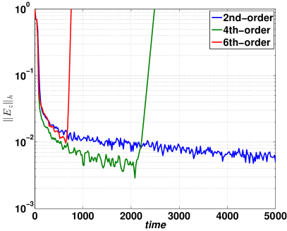
(a) Discrete modal PML (31a)–(31d).

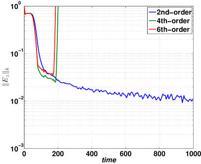
(b) Discrete physically motivated PML (32a)–(32d).

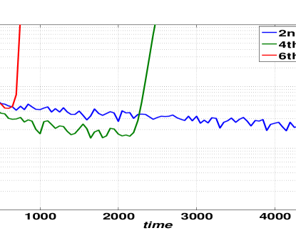
(c) Discrete split–field PML (33a)–(33d).

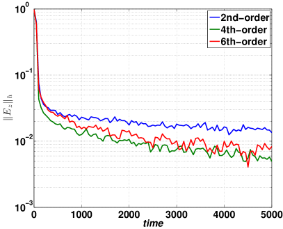
(d) No PML $(\sigma=0)$.

Fig. 1: The $l_{2}$-norm of the electric field as a function of time with the time-step $dt=0.4h$

As in [1, 3, 2], it is possible to argue here that the growth seen for the 4th and 6th order accurate schemes are due to instabilities in the continuous PML models. However, in [21], stability analysis of an IVP corresponding to (26a)–(26d) was performed in detail. The result is that the IVP (26a)–(26d) is asymptotically stable. We believe that the instability seen here and, probably, some of the growth observed in [1, 3, 2] are caused by inappropriate numerical boundary treatments in the PML.

To investigate further, we have also performed numerical experiments with smaller time steps or/and spatial steps. In some cases mesh refinement or smaller time step eliminates the growth, but in other cases the instabilities persist, but it occurs at much later times. For instance, using half of the time step, $dt=0.2h$, postpones the initiation of growth until about $t=4000$ for the PML models (26a)–(26d) and (33a)–(33d) with a 4th order accurate SBP operator. While in all other cases growth was not seen for the entire simulation duration. These simulations are a strong indication that the growth observed here is a numerical artifact. In particular, for the discrete physically motivated PML (32a)–(32d), figure 2(b) indicates that the growth seen in figure 1(b) is due to numerical stiffness. Thus, the numerical approximation (32a)–(32d) of the PML may not be suitable for efficient explicit time integration. These results are also consistent with some of the conclusions drawn in [2], which show that growth for PMLs depends on both the discretization used and the PML model.

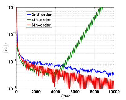
(a) Discrete modal PML (31a)–(31d).

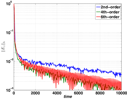
(b) Discrete physically motivated PML (32a)–(32d).

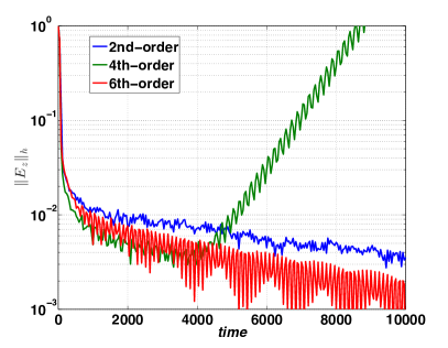
(c) Discrete split–field PML (33a)–(33d).

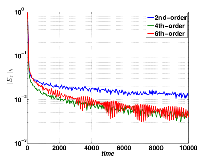
(d) No PML $(\sigma=0)$.

Fig. 2: The $l_{2}$-norm of the electric field as a function of time with the time-step $dt=0.2h$

In the next section, we will show that the IBVPs, (29a)–(29c), (26a)–(26d), (27a)–(27d) and (25a)–(25d) with (3), (2) are also stable. To enable a systematic development of stable numerical boundary procedures we will derive continuous energy estimates. In section 5, by mimicking the continuous energy estimates we will design accurate and stable numerical boundary treatments for the PMLs, (29a)–(29c), (26a)–(26d), (27a)–(27d) and (25a)–(25d), subject to the boundary conditions (5), (2).

4 Continuous analysis

The analysis in [21] shows that the constant coefficient Cauchy PML problem (26a)–(26d) is asymptotically stable. Since the continuous PML models (29a)–(29c), (26a)–(26d), (27a)–(27d) and (25a)–(25d) are equivalent, the results in [21] for the Cauchy problem hold also for the PML models (29a)–(29c), (27a)–(27d) and (25a)–(25d). Note that the boundary condition (3) extends into the PML. In addition the PML is terminated in the $x$–direction by the boundary condition (2). The stability analysis of (29a)–(29c), (26a)–(26d), (27a)–(27d) or (25a)–(25d) subject to the boundary conditions (3) and (2) is not as straightforward. Here, we prove that the PML (29a)–(29c), (26a)–(26d), (27a)–(27d) or (25a)–(25d) with the boundary conditions (3), (2) is stable. First, we will use a modal analysis for a constant coefficient PML. Second, we will derive energy estimates for the variable coefficients case.

4.1 Normal mode analysis

To perform a modal analysis, we assume constant coefficients. We split the PML problem into three: 1) a Cauchy PML problem with no boundary conditions, 2) a lower half–plane PML problem, $-\infty<x<\infty,-\infty<y\leq y_{0}$, with the boundary condition (3) at $y=y_{0}$, and 3) a left half-plane PML problem, $-\infty<x\leq x_{0}+\delta,-\infty<y<\infty$, with the boundary condition (2) at $x=x_{0}+\delta$. Each of the three PML problems above can be analyzed separately. We note that the lower half–plane PML problem and the left half–plane PML problem are distinct and must be analyzed severally.

The Cauchy problem can be analyzed, as in [21], using standard Fourier methods. The analysis in [21] shows that the constant coefficient Cauchy PML problem (29a)–(29c), (26a)–(26d), (27a)–(27d) or (25a)–(25d) is asymptotically stable. As before we have

Theorem 1.

The constant coefficient Cauchy PML problem (29a)–(29c), (26a)–(26d), (27a)–(27d) or (25a)–(25d) with $\sigma\geq 0$ is asymptotically stable.

4.1.1 The lower half–plane PML problem: $-\infty<x<\infty,-\infty<y\leq y_{0}$

Consider now the constant coefficient PML (29a)–(29c), (26a)–(26d), (27a)–(27d) or (25a)–(25d) in a lower half–plane, $-\infty<x<\infty,-\infty<y\leq y_{0}$, with the boundary condition (3) at $y=y_{0}$. Note that the relevant ansatz is no longer a pure Fourier mode, but a simple wave solution on the form

$$\textbf{V}=\widehat{\textbf{V}}(y)e^{st-ik_{x}x},\quad|\widehat{\textbf{V}}(y)|<\infty.$$ (35)

In order to prove the stability of the PML (29a)–(29c), (26a)–(26d), (27a)–(27d) or (25a)–(25d) subject to the boundary condition (3), we will show that the only solution of the form (35) with $\Re{s}\geq 0$ for any $\sigma>0$ is the trivial solution, $\textbf{V}=0$.

To begin with, we introduce the complex number $z=a+ib$ and define the branch cut of $\sqrt{z}$ by

$$-\pi<\arg{\left(a+ib\right)}\leq\pi,\quad\arg{\sqrt{a+ib}}=\frac{1}{2}\arg{{\left(a+ib\right)}}.$$ (36)

Next, we introduce (35) in the PML (29a)–(29c), (26a)–(26d), (27a)–(27d) or (25a)–(25d), and the boundary condition (3). We can eliminate the magnetic fields and the auxiliary variable, then we obtain a second order ODE,

$$\begin{split}\left({s^{2}}+\left(\frac{k_{x}}{1+\frac{\sigma}{s}}\right)^{2}\right)\widehat{E}_{z}=&\frac{d^{2}\widehat{E}_{z}}{dy^{2}},\end{split}$$ (37)

subject to the boundary condition

$$\widehat{H}_{x}+\gamma_{y}\widehat{E}_{z}=0\iff\frac{1}{s}\left(\frac{d\widehat{E}_{z}}{dy}+\gamma_{y}s\widehat{E}_{z}\right)=0,\quad\text{with}\quad\gamma_{y}\geq 0,\quad\text{at}\quad y=y_{0}.$$ (38)

or the PEC boundary condition

$$\widehat{E}_{z}=0,\quad\text{at}\quad y=y_{0}.$$ (39)

Consider now $\Re{s}>0$, we can construct modal solutions, for (37), of the form

$$\widehat{E}_{z}=a_{0}e^{\kappa y}+b_{0}e^{-\kappa y},$$ (40)

where

$$\kappa=\sqrt{s^{2}+\left(\frac{1}{1+\frac{\sigma}{s}}k_{x}\right)^{2}},\quad\Re{s}>0,$$

and $a_{0},b_{0}$ are parameters which must not be zero at the same time. Note that it can be shown that $\Re{\kappa}>0$ for all $\sigma,\Re{s}>0$, see lemma 12 in the appendix. Thus, boundedness of the solutions at $y\to-\infty$ implies $b_{0}=0$. The parameter $a_{0}$ is determined by the boundary condition (38). Introducing (40) in (38) we obtain

$$\frac{a_{0}}{s+\sigma}\left(\sqrt{\left(s+\sigma\right)^{2}+k_{x}^{2}}+\gamma_{y}\left(s+\sigma\right)\right)=0.$$ (41)

Since $a_{0}\neq 0$, we have nontrivial solutions only if

$$\mathcal{F}_{1}\left(s+\sigma,k_{x}\right)\equiv\frac{1}{s+\sigma}\left(\sqrt{\left(s+\sigma\right)^{2}+k_{x}^{2}}+\gamma_{y}\left(s+\sigma\right)\right)=0.$$ (42)

The following lemma characterizes the roots of the dispersion relation (42).

Lemma 2.

Consider the dispersion relation $\mathcal{F}_{1}\left(s+\sigma,k_{x}\right)$ defined in (42) with $\gamma_{y}\geq 0.$ The equation $\mathcal{F}_{1}\left(s+\sigma,k_{x}\right)=0$ has no solution for all $\Re{s}\geq 0$, $k_{x}\in\mathbb{R}$ and $\sigma>0.$

Proof.

Consider first $\sigma=0$, we have $\mathcal{F}_{1}\left(s,k_{x}\right)=0$, with the solution $s=s_{0}\in\mathbb{C}$. Note that since the Maxwell’s equation (1) subject to the boundary conditions (5) satisfy the energy estimate (10) we must have $\Re{s_{0}}\leq 0$, for all $\gamma_{y}\geq 0$. Otherwise if $\Re{s_{0}}>0$, then the energy will grow for some solutions, which is in contradiction with the energy estimate (10). By inspection, the zero root $s_{0}=0$ is also not a solution of $\mathcal{F}_{1}\left(s,k_{x}\right)=0.$

If $\sigma>0$, then the equation $\mathcal{F}_{1}\left(s+\sigma,k_{x}\right)=0$ has the solution $s=-\sigma+s_{0}.$ Therefore, any $\sigma>0$ will move all roots $s$ further into the stable complex plane. ∎

By lemma 2 we must have $\mathcal{F}_{1}\left(s+\sigma,k_{x}\right)\neq 0$ for all $\sigma>0$, $\Re{s}\geq 0$. This also implies that $a_{0}\equiv 0$ in (40) for all $\sigma,\Re{s}>0$. Therefore, the trivial solution is the only possible solution of (26a)–(26d) with (5) or (27a)–(27d) with (5), of the form (35) with $\Re{s}\geq 0$.

Consider now the PEC boundary condition (39) and substitute (40), with $b_{0}\equiv 0$, we have

$$a_{0}=0.$$

Thus the PEC boundary condition (39) supports only trivial solutions, $\textbf{V}=0$.

4.1.2 The left half–plane problem: $-\infty<x\leq x_{0}+\delta,-\infty<y<\infty$

Consider now the constant coefficient PML (29a)–(29c), (26a)–(26d), (27a)–(27d) or (25a)–(25d) in the left half–plane, $-\infty<x\leq x_{0}+\delta,$ $-\infty<y<\infty$, with the boundary condition (2) at $x=x_{0}+\delta$. We make the ansatz

$$\textbf{V}=\widehat{\textbf{V}}(x)e^{st-ik_{y}y},\quad|\widehat{\textbf{V}}(x)|<\infty.$$ (43)

In order to prove the stability of the PML, (29a)–(29c), (26a)–(26d), (27a)–(27d) or (25a)–(25d), subject to the boundary condition (2), we will show that there are no nontrivial solutions on the form (43) with $\Re{s}>0$ for any $\sigma\geq 0$. We insert (43) in (29a)–(29c), (26a)–(26d), (27a)–(27d) or (25a)–(25d) and in the boundary condition (2). As before, we eliminate the magnetic fields and the auxiliary variable to obtain a second order ordinary differential equation,

$$\begin{split}\left({s^{2}}+k_{y}^{2}\right)\widehat{E}_{z}=&\left(\frac{1}{1+\frac{\sigma}{s}}\right)^{2}\frac{d^{2}\widehat{E}_{z}}{dx^{2}},\end{split}$$ (44)

subject to the boundary conditions

$$\widehat{H}_{y}-\gamma_{x}\widehat{E}_{z}=0\iff\frac{1}{s}\left(\left(\frac{1}{1+\frac{\sigma}{s}}\right)\frac{d\widehat{E}_{z}}{dx}+s\gamma_{x}\widehat{E}_{z}\right)=0,\quad\text{with}\quad\gamma_{x}\geq 0,\quad\text{at}\quad x=x_{0}+\delta,$$ (45)

or the PEC boundary condition

$$\widehat{E}_{z}=0,\quad\text{at}\quad x=x_{0}+\delta.$$ (46)

Consider now $\Re{s}>0$, we can construct modal solutions, for (44), on the form

$$\widehat{E}_{z}=a_{0}e^{\kappa x}+b_{0}e^{-\kappa x},$$ (47)

where

$$\kappa=\left({1+\frac{\sigma}{s}}\right)\sqrt{s^{2}+k_{y}^{2}},\quad\Re{s}>0,$$

and $a_{0},b_{0}$ are parameters which must not be zero at the same time. Note that it can be shown that $\Re{\kappa}>0$ for all $\sigma,\Re{s}>0$, see lemma 13 in the appendix. Thus, boundedness of the solution (47) at $x\to-\infty$ implies $b_{0}=0$. The parameter $a_{0}$ is determined by the boundary condition (45). Introducing (47) in (45) we obtain

$$\frac{a_{0}}{s}\left(\sqrt{s^{2}+k_{y}^{2}}+s\right)=0.$$ (48)

Since $a_{0}\neq 0$, we have nontrivial solutions only if

$$\mathcal{F}_{2}\left(s,k_{y}\right)\equiv\frac{1}{s}\left(\sqrt{s^{2}+k_{y}^{2}}+\gamma_{x}s\right)=0.$$ (49)

It is particularly important to note that the dispersion relation $\mathcal{F}_{2}\left(s,k_{y}\right)$, defined by (49), is independent of the PML parameter $\sigma\geq 0$. The dispersion relation (49) corresponds to that of the undamped problem, and it is not perturbed by the PML. This is unlike the dispersion relation, $\mathcal{F}_{1}\left(s+\sigma,k_{y}\right)$ for the lower half–plane PML problem, which depends on the PML parameter $\sigma\geq 0$.

Since, the Maxwell’s equation (1) subject to the boundary conditions (2) and (5) satisfy the energy estimate (10), the following lemma characterizing the roots of the dispersion relation (49) holds

Lemma 3.

Consider the dispersion relation $\mathcal{F}_{2}\left(s,k_{y}\right)$ defined in (49) with $\gamma_{x}>0$. The equation $\mathcal{F}_{2}\left(s,k_{y}\right)=0$ has no solution $s$ for all $\Re{s}\geq 0$ and $k_{y}\in\mathbb{R}$.

Proof.

Since the Maxwell’s equation (1) with the boundary condition (2) at $x=x_{0}+\delta$ satisfy the energy estimate (10) we must have $\Re{s}\leq 0$, for all $k_{y}\in\mathbb{R}$. Otherwise if $\Re{s}>0$, then the energy will grow for some solutions, which is also in contradiction with the energy estimate (10). Again by inspection, the zero root $s=0$ is not a solution of $\mathcal{F}_{2}\left(s,k_{y}\right)=0.$ Note that if $k_{y}=0$ we have $\mathcal{F}_{2}\left(s,k_{y}\right)=1+\gamma_{x}\neq 0$. Next, we consider the case $s=i\xi$, $\xi\in\mathbb{R}/\{0\}$, and introduce $\bar{\xi}=\xi/k_{y}$

$$\mathcal{F}_{2}\left(s,k_{y}\right)\equiv\frac{1}{s}\left(\sqrt{s^{2}+k_{y}^{2}}+\gamma_{x}s\right)=0\iff\mathcal{F}_{0}\left(\bar{\xi}\right)\equiv\sqrt{1-\frac{1}{\bar{\xi^{2}}}}+\gamma_{x}=0.$$ (50)

If $\bar{\xi^{2}}>1$, then we have $\mathcal{F}_{0}\left(\bar{\xi}\right)\neq 0$ since the square root can never be negative. If $\bar{\xi^{2}}\leq 1$, then we also have $\mathcal{F}_{0}\left(\bar{\xi}\right)\neq 0$ since the square root is zero or purely imaginary. Therefore, we must have $\Re{s}<0$, for all $k_{y}\in\mathbb{R}$. This completes the proof of the lemma. ∎

As before, for $\Re{s}\geq 0$ the trivial solution is the only possible solution of (26a)–(26d) with (2) or (27a)–(27d) with (2), on the form (43).

Consider now the PEC boundary condition (39) and substitute (47), with $b_{0}\equiv 0$, we have

$$a_{0}=0.$$

The PEC boundary condition (46) also supports only trivial solutions, $\textbf{V}=0$.

By theorem 1, and lemmas 2 and 3, it then follows that all non–trivial modes in the PML decay. The difficulty lies in constructing accurate and stable numerical approximations for the PML, (29a)–(29c), (26a)–(26d), (27a)–(27d) or (25a)–(25d) subject to the boundary conditions (2) and (5), and ensuring numerical stability.

4.2 Energy equation in the Laplace space

Consider now the constant coefficient PML (29a)–(29c), (26a)–(26d), (27a)–(27d) or (25a)–(25d) in the rectangular domain, $-(x_{0}+\delta)\leq x\leq(x_{0}+\delta),-y_{0}\leq y\leq y_{0}$, and the boundary conditions (3), (2). We will prove that the corresponding constant coefficient IBVP can not support growing modes.

To begin, we assume homogeneous initial data and take the Laplace transform of the PML equations and boundary conditions in time. We can eliminate the magnetic fields and all the auxiliary variables, we have

$$\begin{split}{s^{2}}\widehat{E}_{z}=&\frac{1}{S_{x}}\frac{\partial}{\partial x}\left(\frac{1}{S_{x}}\frac{\partial\widehat{E}_{z}}{\partial x}\right)+\frac{\partial^{2}\widehat{E}_{z}}{\partial y^{2}},\quad\Re{s}>0,\end{split}$$ (51)

subject to the boundary conditions

$$\widehat{H}_{y}\mp\gamma_{x}\widehat{E}_{z}=0\iff\frac{1}{s}\left(\frac{1}{S_{x}}\frac{d\widehat{E}_{z}}{dx}\pm\gamma_{x}s\widehat{E}_{z}\right)=0,\quad\text{at}\quad x=\pm(x_{0}+\delta),$$ (52)

$$\widehat{H}_{x}\pm\gamma_{x}\widehat{E}_{z}=0\iff\frac{1}{s}\left(\frac{d\widehat{E}_{z}}{dy}\pm\gamma_{x}s\widehat{E}_{z}\right)=0,\quad\text{at}\quad y=\pm y_{0}.$$ (53)

or

$$\widehat{E}_{z}=0,\quad\text{at}\quad x=\pm(x_{0}+\delta),$$ (54)

$$\widehat{E}_{z}=0,\quad\text{at}\quad y=\pm y_{0}.$$ (55)

We define the quantity

$$\widehat{\mathcal{E}}_{\sigma}(s)= \Re{s}\|s\widehat{E}_{z}\|^{2}+\Re{\left(\frac{(sS_{x})^{*}}{S_{x}}\right)}\Big{\|}\frac{1}{S_{x}}\frac{\partial{\widehat{E}_{z}}}{\partial x}\Big{\|}^{2}+\Re{s}\Big{\|}\frac{\partial{\widehat{E}_{z}}}{\partial y}\Big{\|}^{2}+\gamma_{y}\left(\|s\widehat{E}_{z}\left(y_{0}\right)\|^{2}_{\Gamma_{x}}+\|s\widehat{E}_{z}\left(-y_{0}\right)\|^{2}_{\Gamma_{x}}\right)$$

$$+\gamma_{x}\Re{\left(\frac{1}{S_{x}}\right)}\left(\|s\widehat{E}_{z}\left(x_{0}+\delta\right)\|^{2}_{\Gamma_{y}}+\|s\widehat{E}_{z}\left(-x_{0}-\delta\right)\|^{2}_{\Gamma_{y}}\right).$$ (56)

For the PEC boundary conditions (54), (55), the boundary terms vanish and we have

$$\widehat{\mathcal{E}}^{0}_{\sigma}(s)= \Re{s}\|s\widehat{E}_{z}\|^{2}+\Re{\left(\frac{(sS_{x})^{*}}{S_{x}}\right)}\Big{\|}\frac{1}{S_{x}}\frac{\partial{\widehat{E}_{z}}}{\partial x}\Big{\|}^{2}+\Re{s}\Big{\|}\frac{\partial{\widehat{E}_{z}}}{\partial y}\Big{\|}^{2}.$$ (57)

Note that $\Re{s}>0\implies\Re{\left(\frac{(sS_{x})^{*}}{S_{x}}\right)},\Re{\left(\frac{1}{S_{x}}\right)}>0$, see lemma 14 in the Appendix. Therefore, $\widehat{\mathcal{E}}_{\sigma}(s)>0$ and $\widehat{\mathcal{E}}^{0}_{\sigma}(s)>0$ are energies. Note also that for $\gamma_{x}\geq 0$, $\gamma_{y}\geq 0$ we have

$$\widehat{\mathcal{E}}_{\sigma}(s)=0\iff\widehat{E}_{z}=\frac{\partial{\widehat{E}_{z}}}{\partial x}=\frac{\partial{\widehat{E}_{z}}}{\partial y}=0,$$

and

$$\widehat{\mathcal{E}}^{0}_{\sigma}(s)=0\iff\widehat{E}_{z}=\frac{\partial{\widehat{E}_{z}}}{\partial x}=\frac{\partial{\widehat{E}_{z}}}{\partial y}=0.$$

We can now prove the theorem:

Theorem 4.

For any $s$, with $\Re{s}>0$, and $\sigma>0,$ all solutions $\widehat{E}_{z}\neq 0$ of the constant coefficient PML (51) in the rectangular domain, with the boundary conditions (52), (53) or (54), (55) must satisfy

$$\begin{split}\widehat{\mathcal{E}}_{\sigma}(s)=0,\quad\text{or}\quad\widehat{\mathcal{E}}^{0}_{\sigma}(s)=0.\end{split}$$ (58)

Proof.

Multiply equation (51) from the left by $\left(s\widehat{{E}}_{z}\right)^{*}$, and integrate over the whole domain, we have

$$\left(s^{2}\widehat{E}_{z},s\widehat{E}_{z}\right)=\left(\frac{1}{S_{x}}\frac{\partial}{\partial x}\left(\frac{1}{S_{x}}\frac{\partial\widehat{E}_{z}}{\partial x}\right),s\widehat{E}_{z}\right)+\left(\frac{d^{2}\widehat{E}_{z}}{dy^{2}},s\widehat{E}_{z}\right)$$ (59)

Integrating by parts and using the boundary conditions (52), (53) obtaining

$$s\left(s\widehat{E}_{z},s\widehat{E}_{z}\right) =-\frac{\left(sS_{x}\right)^{*}}{S_{x}}\left(\frac{1}{S_{x}}\frac{\partial\widehat{E}_{z}}{\partial x},\frac{1}{S_{x}}\frac{\partial\widehat{E}_{z}}{\partial x}\right)-s^{*}\left(\frac{\partial\widehat{E}_{z}}{\partial y},\frac{\partial\widehat{E}_{z}}{\partial y}\right)-\gamma_{y}\left(s\widehat{E}_{z}\left(-y_{0}\right),s\widehat{E}_{z}\left(-y_{0}\right)\right)_{\Gamma_{x}}-\gamma_{y}\left(s\widehat{E}_{z}\left(y_{0}\right),s\widehat{E}_{z}\left(y_{0}\right)\right)_{\Gamma_{x}}$$

$$-\frac{\gamma_{x}}{S_{x}}\left(s\widehat{E}_{z}\left(-x_{0}-\delta\right),s\widehat{E}_{z}\left(-x_{0}-\delta\right)\right)_{\Gamma_{y}}-\frac{\gamma_{x}}{S_{x}}\left(s\widehat{E}_{z}\left(x_{0}+\delta\right),s\widehat{E}_{z}\left(x_{0}+\delta\right)\right)_{\Gamma_{y}}.$$ (60)

We add the complex conjugates of the products in (4.2) to obtain

$$\Re{s}\|s\widehat{E}_{z}\|^{2}+\Re{\left(\frac{(sS_{x})^{*}}{S_{x}}\right)}\Big{\|}\frac{1}{S_{x}}\frac{\partial{\widehat{E}_{z}}}{\partial x}\Big{\|}^{2}+\Re{s}\Big{\|}\frac{\partial{\widehat{E}_{z}}}{\partial y}\Big{\|}^{2}+\gamma_{y}\left(\|s\widehat{E}_{z}\left(y_{0}\right)\|^{2}_{\Gamma_{x}}+\|s\widehat{E}_{z}\left(-y_{0}\right)\|^{2}_{\Gamma_{x}}\right)$$

$$+\gamma_{x}\Re{\left(\frac{1}{S_{x}}\right)}\left(\|s\widehat{E}_{z}\left(x_{0}+\delta\right)\|^{2}_{\Gamma_{y}}+\|s\widehat{E}_{z}\left(-x_{0}-\delta\right)\|^{2}_{\Gamma_{y}}\right)=0.$$ (61)

Note that in particular if the PEC boundary conditions (54), (55) are imposed, the boundary terms vanish and

$$\Re{s}\|s\widehat{E}_{z}\|^{2}+\Re{\left(\frac{(sS_{x})^{*}}{S_{x}}\right)}\Big{\|}\frac{1}{S_{x}}\frac{\partial{\widehat{E}_{z}}}{\partial x}\Big{\|}^{2}+\Re{s}\Big{\|}\frac{\partial{\widehat{E}_{z}}}{\partial y}\Big{\|}^{2}=0.$$ (62)

Thus, for $\Re{s}>0$ no nontrivial solutions $\widehat{E}_{z}\neq 0$ can be supported by the PML. ∎

4.3 Energy estimates in the time domain

To enable the development of a systematic and rigorous stable numerical boundary procedure for the time–dependent PML we will derive energy estimates for the variable coefficient PML. The importance of the energy estimates are twofold: The first is that the energy estimates establish the well–posedness of the variable coefficients PMLs. The second is that by mimicking the energy estimates we can construct high order accurate, stable and convergent discrete approximations of the PML in a bounded domain.

4.3.1 Energy estimates for the modal PML

The first step is to rewrite the PML (26a)–(26d) and the boundary conditions (3), (2) as a second order system. Differentiating equation (26a) with respect to time and using equations (26b)–(26d) to eliminate the time–derivatives on the right hand side, we obtain

$$\frac{\partial^{2}{E_{z}}}{\partial t^{2}}+\sigma\frac{\partial{E_{z}}}{\partial t} =\frac{\partial}{\partial x}\left(\frac{\partial{E_{z}}}{\partial x}+\sigma H_{y}\right)+\frac{\partial}{\partial y}\left(\frac{\partial{E_{z}}}{\partial y}+\sigma H_{x}\right),$$ (63a)

$$\frac{\partial{H_{y}}}{\partial t} =-\frac{\partial{E_{z}}}{\partial x}-\sigma H_{y},$$ (63b)

$$\frac{\partial{H_{x}}}{\partial t} =\frac{\partial{E_{z}}}{\partial y}.$$ (63c)

The corresponding boundary conditions are

$$\gamma_{x}E_{z}\pm H_{x}=0\implies\gamma_{x}\frac{\partial{E_{z}}}{\partial t}+\sigma\gamma_{x}E_{z}\pm\left(\frac{\partial{E_{z}}}{\partial y}+\sigma H_{x}\right)=0,\quad\text{at}\quad y=\pm y_{0}.$$ (64)

$$\gamma_{y}E_{z}\mp H_{y}=0,\implies\gamma_{y}\frac{\partial{E_{z}}}{\partial t}\pm\left(\frac{\partial{E_{z}}}{\partial x}+\sigma H_{y}\right)=0,\quad\text{at}\quad x=\pm(x_{0}+\delta).$$ (65)

or

$$E_{z}=0,\implies\frac{\partial{E_{z}}}{\partial t}=0,\quad\text{at}\quad y=\pm y_{0}.$$ (66)

$$E_{z}=0,\implies\frac{\partial{E_{z}}}{\partial t}=0,\quad\text{at}\quad x=\pm(x_{0}+\delta).$$ (67)

Here, the length and width of the computational domain are $\Gamma_{x}:=\{x:-x_{0}-\delta\leq x\leq x_{0}+\delta\}$ and $\Gamma_{y}:=\{y:-y_{0}\leq y\leq y_{0}\}$, respectively. To derive an energy estimate we introduce the relevant energy norms

$$\begin{split}\mathcal{E}_{\sigma}^{\left(1\right)}\left(t\right)&=\Big{\|}\frac{\partial{E_{z}}}{\partial t}\Big{\|}^{2}+\Big{\|}\frac{\partial{E_{z}}}{\partial x}+\sigma H_{y}\Big{\|}^{2}+\Big{\|}\frac{\partial{E_{z}}}{\partial y}+\sigma H_{x}\Big{\|}^{2}+\Big{\|}\sigma H_{y}\Big{\|}^{2}+\Big{\|}\sigma H_{x}\Big{\|}^{2}+\gamma\sigma\left\|E_{z}\left(-y_{0},\mathrm{t}^{\prime}\right)\right\|^{2}_{\Gamma_{x}}+\gamma\sigma\left\|E_{z}\left(y_{0},\mathrm{t}^{\prime}\right)\right\|^{2}_{\Gamma_{x}}\\ &+\int_{0}^{t}\left(\gamma_{x}\left\|\frac{\partial{E_{z}}}{\partial t}\left(-y_{0},\mathrm{t}^{\prime}\right)\right\|^{2}_{\Gamma_{x}}+\gamma_{x}\left\|\frac{\partial{E_{z}}}{\partial t}\left(y_{0},\mathrm{t}^{\prime}\right)\right\|^{2}_{\Gamma_{x}}+\gamma_{y}\left\|\frac{\partial{E_{z}}}{\partial t}\left(x_{0}+\delta,\mathrm{t}^{\prime}\right)\right\|^{2}_{\Gamma_{y}}+\gamma_{y}\left\|\frac{\partial{E_{z}}}{\partial t}\left(-x_{0}-\delta,\mathrm{t}^{\prime}\right)\right\|^{2}_{\Gamma_{y}}\right)\mathrm{dt}^{\prime},\end{split}$$ (68)

and

$$\begin{split}\mathcal{E}_{\sigma}^{\left(0\right)}\left(t\right)&=\Big{\|}\frac{\partial{E_{z}}}{\partial t}\Big{\|}^{2}+\Big{\|}\frac{\partial{E_{z}}}{\partial x}+\sigma H_{y}\Big{\|}^{2}+\Big{\|}\frac{\partial{E_{z}}}{\partial y}+\sigma H_{x}\Big{\|}^{2}+\Big{\|}\sigma H_{y}\Big{\|}^{2}+\Big{\|}\sigma H_{x}\Big{\|}^{2}.\end{split}$$ (69)

Note that away from the boundaries, the energy norm (68) is analogous to the norms derived in [22, 17]. The difference between (68) and [22, 17] is that the energy norm introduced here contains also boundary norms, $\|\cdot\|_{\Gamma_{x}}$, $\|\cdot\|_{\Gamma_{y}}$. Note also that $\mathcal{E}_{\sigma}^{\left(1\right)}\left(t\right)=0$, $\mathcal{E}_{\sigma}^{\left(0\right)}\left(t\right)=0$, if and only if

$$\frac{\partial{E_{z}}}{\partial t}=\frac{\partial{E_{z}}}{\partial x}=\frac{\partial{E_{z}}}{\partial y}=\sigma H_{x}=\sigma H_{y}=0.$$

When the damping vanishes, $\sigma=0$, we have the physical energy norms

$$\begin{split}\mathcal{E}^{\left(1\right)}\left(t\right)&=\Big{\|}\frac{\partial{E_{z}}}{\partial t}\Big{\|}^{2}+\Big{\|}\frac{\partial{E_{z}}}{\partial x}\Big{\|}^{2}+\Big{\|}\frac{\partial{E_{z}}}{\partial y}\Big{\|}^{2}\\ &+2\int_{0}^{t}\left(\gamma_{x}\left\|\frac{\partial{E_{z}}}{\partial t}\left(-y_{0},\mathrm{t}^{\prime}\right)\right\|^{2}_{\Gamma_{x}}+\gamma_{x}\left\|\frac{\partial{E_{z}}}{\partial t}\left(y_{0},\mathrm{t}^{\prime}\right)\right\|^{2}_{\Gamma_{x}}+\gamma_{y}\left\|\frac{\partial{E_{z}}}{\partial t}\left(x_{0}+\delta,\mathrm{t}^{\prime}\right)\right\|^{2}_{\Gamma_{y}}+\gamma_{y}\left\|\frac{\partial{E_{z}}}{\partial t}\left(-x_{0}-\delta,\mathrm{t}^{\prime}\right)\right\|^{2}_{\Gamma_{y}}\right)\mathrm{dt}^{\prime},\end{split}$$ (70)

and

$$\begin{split}\mathcal{E}^{\left(0\right)}\left(t\right)&=\Big{\|}\frac{\partial{E_{z}}}{\partial t}\Big{\|}^{2}+\Big{\|}\frac{\partial{E_{z}}}{\partial x}\Big{\|}^{2}+\Big{\|}\frac{\partial{E_{z}}}{\partial y}\Big{\|}^{2}.\end{split}$$ (71)

Let us define the spaces of real functions

$$\mathbf{\mathcal{V}}_{\mathcal{E}^{\left(1\right)}}:=\{E_{z}:\mathcal{E}^{\left(1\right)}<\infty\},\quad\mathbf{\mathcal{V}}_{\mathcal{E}_{\sigma}^{\left(1\right)}}:=\{\left(E_{z},H_{x},H_{y}\right):\mathcal{E}_{\sigma}^{\left(1\right)}<\infty\},$$ (72)

$$\mathbf{\mathcal{V}}_{\mathcal{E}^{\left(0\right)}}:=\{E_{z}:\mathcal{E}^{\left(0\right)}<\infty\},\quad\mathbf{\mathcal{V}}_{\mathcal{E}_{\sigma}^{\left(0\right)}}:=\{\left(E_{z},H_{x},H_{y}\right):\mathcal{E}_{\sigma}^{\left(0\right)}<\infty\},$$ (73)

and $L^{2}\left(\Omega\right)$ the space of square integrable real functions. It can be shown that

$$\left(E_{z},H_{x},H_{y}\right)\in\mathbf{\mathcal{V}}_{\mathcal{E}_{\sigma}^{\left(1\right)}}\iff\{E_{z}\in\mathbf{\mathcal{V}}_{\mathcal{E}^{\left(1\right)}},\quad\left(H_{x},H_{y}\right)\in L^{2}\left(\Omega\right)\},$$ (74)

and

$$\left(E_{z},H_{x},H_{y}\right)\in\mathbf{\mathcal{V}}_{\mathcal{E}_{\sigma}^{\left(0\right)}}\iff\{E_{z}\in\mathbf{\mathcal{V}}_{\mathcal{E}^{\left(0\right)}},\quad\left(H_{x},H_{y}\right)\in L^{2}\left(\Omega\right)\}.$$ (75)

We can now prove the theorem, see Appendix B:

Theorem 5.

All solutions of the perfectly matched layer (26a)–(26d) or (63a)–(63c) subject to the boundary conditions (64) at $y=\pm y_{0}$ and (65) at $x=\pm x_{0}$, or (66) at $y=\pm y_{0}$ and (67) at $x=\pm x_{0}$ satisfies the energy estimate

$$\begin{split}\frac{\mathrm{d}}{\mathrm{dt}}\sqrt{\mathcal{E}_{\sigma}^{\left(1\right)}\left(\mathrm{t}\right)}\leq{\sigma_{\infty}}\sqrt{\mathcal{E}_{\sigma}^{\left(1\right)}\left(t\right)},\quad\text{or}\quad\frac{\mathrm{d}}{\mathrm{dt}}\sqrt{\mathcal{E}_{\sigma}^{\left(0\right)}\left(\mathrm{t}\right)}\leq{\sigma_{\infty}}\sqrt{\mathcal{E}_{\sigma}^{\left(0\right)}\left(t\right)},\end{split}$$ (76)

where $\sigma_{\infty}=\max_{x}\sigma(x).$

Remark 2.

It is particularly noteworthy that the PML models (29a)–(29c) and (25a)–(25d) can be rewritten directly in the time domain as (26a)–(26d). Therefore, theorem 5 holds also for the solutions of (29a)–(29c) and (25a)–(25d).

In the next section, by mimicking the continuous energy estimate (76), we will develop stable numerical boundary procedures for the PML models (29a)–(29c), (26a)–(26d) and (25a)–(25d), subject to the boundary conditions (64) at $y=\pm y_{0}$ and (65) at $x=\pm(x_{0}+\delta)$.

4.3.2 Energy estimates for the physically motivated PML

The physically motivated PML model (27a)–(27d), satisfies the definition of a strongly hyperbolic system. By applying the energy method directly to the PML, (27a)–(27d), subject to the boundary conditions (4), (5), with $\gamma_{j}\geq 0$, we have

$$\begin{split}&\frac{d}{dt}\left(\|E_{z}\left(t\right)\|^{2}+\|H_{y}\left(t\right)\|^{2}+\|H_{x}\left(t\right)\|^{2}+\|P\left(t\right)\|^{2}\right)=-2\sigma\|E_{z}\left(t\right)\|^{2}-2\sigma\|H_{y}\left(t\right)\|^{2}+2\sigma\|H_{x}\left(t\right)\|^{2}-2\sigma\|P\left(t\right)\|^{2}\\ &-2\gamma_{x}\left(\|E_{z}\left(t,x_{0}+\delta\right)\|^{2}_{\Gamma_{y}}+\|E_{z}\left(t,-x_{0}-\delta\right)\|^{2}_{\Gamma_{y}}\right)-2\gamma_{y}\ \left(\|E_{z}\left(t,y_{0}\right)\|^{2}_{\Gamma_{x}}+\|E_{z}\left(t,-y_{0}\right)\|^{2}_{\Gamma_{x}}\right).\end{split}$$ (77)

In particular if $\gamma_{j}=0$ in (4), (5) or $R_{j}=-1$ (we consider the PEC condition) in (2), (3) then

$$\begin{split}&\frac{d}{dt}\left(\|E_{z}\left(t\right)\|^{2}+\|H_{y}\left(t\right)\|^{2}+\|H_{x}\left(t\right)\|^{2}+\|P\left(t\right)\|^{2}\right)=-2\sigma\|E_{z}\left(t\right)\|^{2}-2\sigma\|H_{y}\left(t\right)\|^{2}+2\sigma\|H_{x}\left(t\right)\|^{2}-2\sigma\|P\left(t\right)\|^{2}.\end{split}$$ (78)

Note that all terms, excepting $+2\sigma\|H_{x}\left(t\right)\|^{2}$, in the right hand sides of (77), (78) are dissipative. We denote the energy by

$$\begin{split}\mathcal{E}^{(2)}\left(\mathrm{t}\right)&=\|E_{z}\left(t\right)\|^{2}+\|H_{y}\left(t\right)\|^{2}+\|H_{x}\left(t\right)\|^{2}+\|P\left(t\right)\|^{2}\\ &+2\int_{0}^{t}\left(\gamma_{x}\left(\|E_{z}\left(t^{\prime},x_{0}+\delta\right)\|^{2}_{\Gamma_{y}}+\|E_{z}\left(t^{\prime},-x_{0}-\delta\right)\|^{2}_{\Gamma_{y}}\right)+\gamma_{y}\ \left(\|E_{z}\left(t^{\prime},y_{0}\right)\|^{2}_{\Gamma_{x}}+\|E_{z}\left(t^{\prime},-y_{0}\right)\|^{2}_{\Gamma_{x}}\right)\right)\mathrm{dt}^{\prime},\end{split}$$ (79)

and

$$\begin{split}\mathcal{E}^{(2)}_{0}\left(\mathrm{t}\right)&=\|E_{z}\left(t\right)\|^{2}+\|H_{y}\left(t\right)\|^{2}+\|H_{x}\left(t\right)\|^{2}+\|P\left(t\right)\|^{2},\end{split}$$ (80)

if $\gamma_{j}=0$ in (4), (5) or $R_{j}=-1$ (we consider the PEC condition) in (2). We have

Theorem 6.

The solutions of the perfectly matched layer (27a)–(27d) subject to the boundary conditions (4), (5) with $|R_{j}|<1$ or $|R_{j}|=1$ satisfy the energy estimate

$$\begin{split}\frac{\mathrm{d}}{\mathrm{dt}}\sqrt{\mathcal{E}^{\left(2\right)}\left(\mathrm{t}\right)}\leq\sigma_{\infty}\sqrt{\mathcal{E}^{\left(2\right)}\left(t\right)},\quad\text{or}\quad\frac{\mathrm{d}}{\mathrm{dt}}\sqrt{\mathcal{E}_{0}^{\left(2\right)}\left(\mathrm{t}\right)}\leq\sigma_{\infty}\sqrt{\mathcal{E}_{0}^{\left(2\right)}\left(t\right)},\end{split}$$ (81)

where $\sigma_{\infty}=\max_{x}\sigma(x).$

5 Discrete approximations and discrete stability analysis of the PMLs

The main focus of this section is to design accurate, stable and efficient numerical boundary procedures for the PMLs, (29a)–(29c), (26a)–(26d),(25a)–(25d) and (27a)–(27d), subject to the boundary conditions (3), (2). We will use SBP finite difference operators, see [26, 48], to approximate the spatial derivatives and impose boundary conditions weakly using penalties [15, 43]. To ensure numerical stability we will impose boundary conditions in a manner which allows a derivation of discrete energy estimates analogous to the continuous energy estimate (76). For the physically motivated PML model (27a)–(27d), an efficient numerical boundary treatment is achieved by using characteristics and reducing the strength of the penalty parameters. Finally, we will show that the corresponding discrete models do not support growing modes.

5.1 Discrete approximation and discrete energy estimates for the modal PML

In standard numerical methods [3, 2, 10], once the interior scheme is proven stable the discrete PML is obtained by discretizing the auxiliary differential equations and appending the auxiliary functions accordingly. Usually no more attention is placed on how the boundary conditions are implemented in the PML. Note that numerical experiments presented in section 3 and the next section show that a straightforward enforcement of the boundary conditions, (3) and (2), can lead to unstable solutions in the PML. A stable discrete approximation for the modal PML can be obtained by extending the enforcement of the boundary condition to the auxiliary differential equation, having

$$\frac{\mathrm{d}{\mathbf{E}_{z}}}{\mathrm{dt}} =-\left(D_{x}\otimes I_{y}\right)\mathbf{H}_{y}+\left(I_{x}\otimes D_{y}\right)\mathbf{H}_{x}+\mathbf{H}_{x}^{*}-\mathbf{\sigma}\mathbf{E}_{z}$$

$$\underbrace{-\alpha_{x}\left(\frac{1-R_{x}}{2}\left(\mathrm{P}_{x}^{-1}\left(E_{Rx}+E_{Lx}\right)\otimes I_{y}\right)\mathbf{E}_{z}-\frac{1+R_{x}}{2}\left(\mathrm{P}_{x}^{-1}\left(E_{Rx}-E_{Lx}\right)\otimes I_{y}\right)\mathbf{H}_{y}\right)}_{\mathrm{SAT}_{x}}$$

$$\underbrace{-\alpha_{y}\left(\frac{1-R_{y}}{2}\left(I_{x}\otimes\mathrm{P}_{y}^{-1}\left(E_{Ry}+E_{Ly}\right)\right)\mathbf{E}_{z}+\frac{1+R_{y}}{2}\left(I_{x}\otimes\mathrm{P}_{y}^{-1}\left(E_{Ry}-E_{Ly}\right)\right)\mathbf{H}_{x}\right)}_{\mathrm{SAT}_{y}},$$ (82a)

$$\frac{\mathrm{d}{\mathbf{H}_{y}}}{\mathrm{dt}} =-\left(D_{x}\otimes I_{y}\right)\mathbf{E}_{z}-\mathbf{\sigma}\mathbf{H}_{y}\underbrace{+\theta_{x}\left(\frac{1-R_{x}}{2}\left(\mathrm{P}_{x}^{-1}\left(E_{Rx}-E_{Lx}\right)\otimes I_{y}\right)\mathbf{E}_{z}-\frac{1+R_{x}}{2}\left(\mathrm{P}_{x}^{-1}\left(E_{Rx}+E_{Lx}\right)\otimes I_{y}\right)\mathbf{H}_{y}\right)}_{\mathrm{SAT}_{x}},$$ (82b)

$$\frac{\mathrm{d}{\mathbf{H}_{x}}}{\mathrm{dt}} =\left(I_{x}\otimes D_{y}\right)\mathbf{E}_{z}\underbrace{-\theta_{y}\left(\frac{1-R_{y}}{2}\left(I_{x}\otimes\mathrm{P}_{y}^{-1}\left(E_{Ry}-E_{Ly}\right)\right)\mathbf{E}_{z}+\frac{1+R_{y}}{2}\left(I_{x}\otimes\mathrm{P}_{y}^{-1}\left(E_{Ry}+E_{Ly}\right)\right)\mathbf{H}_{x}\right)}_{\mathrm{SAT}_{y}},$$ (82c)

$$\frac{\mathrm{d}{\mathbf{H}_{x}^{*}}}{\mathrm{dt}} =\sigma\left(\left(I_{x}\otimes D_{y}\right)\mathbf{H}_{x}\underbrace{-\theta\alpha_{y}\left(\frac{1-R_{y}}{2}\left(I_{x}\otimes\mathrm{P}_{y}^{-1}\left(E_{Ry}+E_{Ly}\right)\right)\mathbf{E}_{z}+\frac{1+R_{y}}{2}\left(I_{x}\otimes\mathrm{P}_{y}^{-1}\left(E_{Ry}-E_{Ly}\right)\right)\mathbf{H}_{x}\right)}_{\text{Stabilizing term}}\right).$$ (82d)

Note that we have included the term involving $\theta$. The standard choice $\theta=0$, which corresponds to (31a)–(31d), is obtained by simply replacing spatial derivatives with difference operators in the PML. The other choice, $\theta\neq 0$, extends weak enforcements of the boundary conditions, (3) in the $y$-direction, to the auxiliary differential equation (83d). It is particularly important to note that this extension, with $\theta\neq 0$, does not destroy the accuracy of the scheme (83a)–(83d). When $\sigma=0$, the auxiliary variable $\mathbf{H}_{x}^{*}$ also vanishes, and the discrete approximation (83a)–(83d), for any value of $\theta$, correspond to the stable discrete approximation (14a)–(14c). However, as we will see later, when $\sigma>0$ the particular choice $\theta=1$ ensures numerical stability.

To be able to simplify the analysis and also make comparisons with results published in the literature, we will focus on the setup considered in section 3.3 and [1, 3, 2]. Therefore, we set $R_{x}=R_{y}=0$ and the penalty parameters

$$\alpha_{x}=2,\quad\alpha_{y}=2,\quad\theta_{x}=\theta_{y}=0,$$

having

$$\frac{\mathrm{d}{\mathbf{E}_{z}}}{\mathrm{dt}} =-\left(D_{x}\otimes I_{y}\right)\mathbf{H}_{y}+\left(I_{x}\otimes D_{y}\right)\mathbf{H}_{x}+\mathbf{H}_{x}^{*}-\mathbf{\sigma}\mathbf{E}_{z}\underbrace{-\left(\left(\mathrm{P}_{x}^{-1}\left(E_{Rx}+E_{Lx}\right)\otimes I_{y}\right)\mathbf{E}_{z}-\left(\mathrm{P}_{x}^{-1}\left(E_{Rx}-E_{Lx}\right)\otimes I_{y}\right)\mathbf{H}_{y}\right)}_{\mathrm{SAT}_{x}}$$

$$\underbrace{-\left(\left(I_{x}\otimes\mathrm{P}_{y}^{-1}\left(E_{Ry}+E_{Ly}\right)\right)\mathbf{E}_{z}+\left(I_{x}\otimes\mathrm{P}_{y}^{-1}\left(E_{Ry}-E_{Ly}\right)\right)\mathbf{H}_{x}\right)}_{\mathrm{SAT}_{y}},$$ (83a)

$$\frac{\mathrm{d}{\mathbf{H}_{y}}}{\mathrm{dt}} =-\left(D_{x}\otimes I_{y}\right)\mathbf{E}_{z}-\mathbf{\sigma}\mathbf{H}_{y},$$ (83b)

$$\frac{\mathrm{d}{\mathbf{H}_{x}}}{\mathrm{dt}} =\left(I_{x}\otimes D_{y}\right)\mathbf{E}_{z},$$ (83c)

$$\frac{\mathrm{d}{\mathbf{H}_{x}^{*}}}{\mathrm{dt}} =\sigma\left(\left(I_{x}\otimes D_{y}\right)\mathbf{H}_{x}\underbrace{-\theta\left(\left(I_{x}\otimes\mathrm{P}_{y}^{-1}\left(E_{Ry}+E_{Ly}\right)\right)\mathbf{E}_{z}+\left(I_{x}\otimes\mathrm{P}_{y}^{-1}\left(E_{Ry}-E_{Ly}\right)\right)\mathbf{H}_{x}\right)}_{\text{Stabilizing term}}\right).$$ (83d)

5.1.1 Discrete energy estimates in the time domain

We will derive a discrete energy estimate analogous to the continuous energy estimate (76). First and foremost, we rewrite (83a)–(83d) as a second order system. Differentiate equation (83a) in time, and use equations (83b)–(83d) to eliminate the time derivatives in the right hand side. We have

$$\frac{\mathrm{d^{2}}{\mathbf{E}_{z}}}{\mathrm{dt^{2}}} =\left(D_{x}\otimes I_{y}\right)\left(\left(D_{x}\otimes I_{y}\right)\mathbf{E}_{z}+\mathbf{\sigma}\mathbf{H}_{y}\right)+\left(I_{x}\otimes D_{y}\right)\left(I_{x}\otimes D_{y}\right)\mathbf{E}_{z}$$ (84a)

$$+\sigma\left(\left(I_{x}\otimes D_{y}\right)\mathbf{H}_{x}\underbrace{-\theta\left(\left(I_{x}\otimes\mathrm{P}_{y}^{-1}\left(E_{Ry}+E_{Ly}\right)\right)\mathbf{E}_{z}+\left(I_{x}\otimes\mathrm{P}_{y}^{-1}\left(E_{Ry}-E_{Ly}\right)\right)\mathbf{H}_{x}\right)}_{\text{Stabilizing term}}\right)-\mathbf{\sigma}\frac{\mathrm{d}{\mathbf{E}_{z}}}{\mathrm{dt}}$$

$$\underbrace{-\left(\left(\mathrm{P}_{x}^{-1}\left(E_{Rx}+E_{Lx}\right)\otimes I_{y}\right)\frac{\mathrm{d}{\mathbf{E}_{z}}}{\mathrm{dt}}+\left(\mathrm{P}_{x}^{-1}\left(E_{Rx}-E_{Lx}\right)\otimes I_{y}\right)\left(\left(D_{x}\otimes I_{y}\right)\mathbf{E}_{z}+\mathbf{\sigma}\mathbf{H}_{y}\right)\right)}_{\mathrm{SAT}_{x}}$$

$$\underbrace{-\left(\left(I_{x}\otimes\mathrm{P}_{y}^{-1}\left(E_{Ry}+E_{Ly}\right)\right)\frac{\mathrm{d}{\mathbf{E}_{z}}}{\mathrm{dt}}+\left(I_{x}\otimes\mathrm{P}_{y}^{-1}\left(E_{Ry}-E_{Ly}\right)\right)\left(I_{x}\otimes D_{y}\right)\mathbf{E}_{z}\right)}_{\mathrm{SAT}_{y}},$$ (84b)

$$\frac{\mathrm{d}{\mathbf{H}_{y}}}{\mathrm{dt}} =-\left(D_{x}\otimes I_{y}\right)\mathbf{E}_{z}-\mathbf{\sigma}\mathbf{H}_{y},$$ (84c)

$$\frac{\mathrm{d}{\mathbf{H}_{x}}}{\mathrm{dt}} =\left(I_{x}\otimes D_{y}\right)\mathbf{E}_{z},$$ (84d)

Subsequently, by using the SBP property (13) we eliminate some of the SAT terms and obtain

$$\frac{\mathrm{d^{2}}{\mathbf{E}_{z}}}{\mathrm{dt^{2}}} =-\left(\mathrm{P}_{x}^{-1}D_{x}^{T}\otimes I_{y}\right)\left(\mathrm{P}_{x}\otimes I_{y}\right)\left(\left(D_{x}\otimes I_{y}\right)\mathbf{E}_{z}+\mathbf{\sigma}\mathbf{H}_{y}\right)-\left(I_{x}\otimes\mathrm{P}_{y}^{-1}D_{y}^{T}\right)\left(I_{x}\otimes\mathrm{P}_{y}\right)\left(\left(I_{x}\otimes D_{y}\right)\mathbf{E}_{z}+\mathbf{\sigma}\mathbf{H}_{x}\right)-\sigma\frac{\mathrm{d}{\mathbf{E}_{z}}}{\mathrm{dt}}$$

$$+\sigma(1-\theta)\left(I_{x}\otimes\mathrm{P}_{y}^{-1}\left(E_{Ry}-E_{Ly}\right)\right)\mathbf{H}_{x}-\left(\mathrm{P}_{x}^{-1}\left(E_{Rx}+E_{Lx}\right)\otimes I_{y}+\left(I_{x}\otimes\mathrm{P}_{y}^{-1}\left(E_{Ry}+E_{Ly}\right)\right)\right)\frac{\mathrm{d}{\mathbf{E}_{z}}}{\mathrm{dt}}$$

$$-\sigma\theta\left(I_{x}\otimes\mathrm{P}_{y}^{-1}\left(E_{Ry}+E_{Ly}\right)\right)\mathbf{E}_{z},$$ (85a)

$$\frac{\mathrm{d}{\mathbf{H}_{y}}}{\mathrm{dt}} =-\left(D_{x}\otimes I_{y}\right)\mathbf{E}_{z}-\mathbf{\sigma}\mathbf{H}_{y},$$ (85b)

$$\frac{\mathrm{d}{\mathbf{H}_{x}}}{\mathrm{dt}} =\left(I_{x}\otimes D_{y}\right)\mathbf{E}_{z}.$$ (85c)

Introduce the discrete energy

$$\begin{split}\mathcal{E}_{h\sigma}^{(1)}\left(t\right)&=\Big{\|}\frac{\mathrm{d}{\mathbf{E}_{z}}}{\mathrm{dt}}\Big{\|}^{2}_{\mathbf{P}_{xy}}+\Big{\|}\left(D_{x}\otimes I_{y}\right)\mathbf{E}_{z}+\mathbf{\sigma}\mathbf{H}_{y}\Big{\|}^{2}_{\mathbf{P}_{xy}}+\Big{\|}\left(I_{x}\otimes D_{y}\right)\mathbf{E}_{z}+\sigma\mathbf{H}_{x}\Big{\|}^{2}_{\mathbf{P}_{xy}}+\Big{\|}\sigma\mathbf{H}_{y}\Big{\|}^{2}_{\mathbf{P}_{xy}}+\Big{\|}\sigma\mathbf{H}_{x}\Big{\|}^{2}_{\mathbf{P}_{xy}}\\ &+\mathbf{E}_{z}^{T}\left(\mathrm{P}_{x}\otimes\sigma\theta\left(E_{Ry}+E_{Ly}\right)\right)\mathbf{E}_{z}+2\int_{0}^{t}\left(\frac{\mathrm{d}{\mathbf{E}_{z}}}{\mathrm{dt}}^{T}\left(\left(E_{Rx}+E_{Lx}\right)\otimes\mathrm{P}_{y}+\mathrm{P}_{x}\otimes\left(E_{Ry}+E_{Ly}\right)\right)\frac{\mathrm{d}{\mathbf{E}_{z}}}{\mathrm{dt}}\right)dt^{\prime}.\end{split}$$ (86)

When $\sigma=0$ we have the standard discrete energy

$$\begin{split}\mathcal{E}_{h}^{(1)}\left(t\right)&=\Big{\|}\frac{\mathrm{d}{\mathbf{E}_{z}}}{\mathrm{dt}}\Big{\|}^{2}_{\mathbf{P}_{xy}}+\Big{\|}\left(D_{x}\otimes I_{y}\right)\mathbf{E}_{z}\Big{\|}^{2}_{\mathbf{P}_{xy}}+\Big{\|}\left(I_{x}\otimes D_{y}\right)\mathbf{E}_{z}\Big{\|}^{2}_{\mathbf{P}_{xy}}\\ &+2\int_{0}^{t}\left(\frac{\mathrm{d}{\mathbf{E}_{z}}}{\mathrm{dt}}^{T}\left(\left(E_{Rx}+E_{Lx}\right)\otimes\mathrm{P}_{y}+\mathrm{P}_{x}\otimes\left(E_{Ry}+E_{Ly}\right)\right)\frac{\mathrm{d}{\mathbf{E}_{z}}}{\mathrm{dt}}\right)dt^{\prime}.\end{split}$$ (87)

We can also prove the following, see Appendix C.

Theorem 7.

Consider the discrete approximation (83a)–(83d) or (85a)–(85c) of the the perfectly matched layer (26a)–(26d) subject to the boundary conditions (64) at $y=\pm y_{0}$ and (65) at $x=\pm x_{0}$. If $\theta=1$, then the quantity $\mathcal{E}_{h\sigma}\left(t\right)$ defined in (86) is an energy and the solutions of the discrete system (83a)–(83d) or (85a)–(85c) satisfy the energy estimate

$$\begin{split}\frac{\mathrm{d}}{\mathrm{dt}}\sqrt{\mathcal{E}_{h\sigma}^{(1)}\left(t\right)}\leq&\sigma_{\infty}\sqrt{\mathcal{E}_{h\sigma}^{(1)}\left(t\right)}.\end{split}$$ (88)

Note that when $\sigma=0$ we have a strict energy estimate

$$\begin{split}\frac{\mathrm{d}}{\mathrm{dt}}\sqrt{\mathcal{E}_{h\sigma}^{(1)}\left(t\right)}\leq&0,\end{split}$$ (89)

for any values of $\theta$. However, for $\sigma\geq 0$, if $\theta\neq 1$ we are unable to derive a discrete energy estimate for the discrete PML. In standard numerical codes, as shown in section 3, once the interior scheme is proven stable, the PML is then added as lower order modification, leading to the standard choice $\theta=0$. If $\theta\neq 1$, then there is a non-vanishing boundary term,

$$\sigma(1-\theta)\left(I_{x}\otimes\mathrm{P}_{y}^{-1}\left(E_{Ry}-E_{Ly}\right)\right)\mathbf{H}_{x}.$$ (90)

The boundary term (90) will probably diminish with mesh refinement, $h\to 0$. However, on a realistic mesh the boundary term (90) may be nontrivial.

The energy estimate (88) above does not exclude the possibility of exponentially growing solutions for $\sigma>0$. However, the estimate can be extended to the error equations to proof convergence of the solutions of the discrete approximation (83a)–(83d) or (85a)–(85c) for any finite time interval $[0,T]$. Below, we will prove that at constant coefficients the semi–discrete PML problem (83a)–(83d) or (85a)–(85c) can not support exponentially growing solutions.

5.1.2 Discrete energy estimates in the Laplace space

Consider now the semi–discrete system (85a)–(85c) and take the Laplace transform in time, we have

$$s^{2}\widehat{\mathbf{E}}_{z} =-\left(\mathrm{P}_{x}^{-1}D_{x}^{T}\otimes I_{y}\right)\left(\mathrm{P}_{x}\otimes I_{y}\right)\left(\left(D_{x}\otimes I_{y}\right)\widehat{\mathbf{E}}_{z}+\mathbf{\sigma}\widehat{\mathbf{H}}_{y}\right)-\left(I_{x}\otimes\mathrm{P}_{y}^{-1}D_{y}^{T}\right)\left(I_{x}\otimes\mathrm{P}_{y}\right)\left(\left(I_{x}\otimes D_{y}\right)\widehat{\mathbf{E}}_{z}+\mathbf{\sigma}\widehat{\mathbf{H}}_{x}\right)-\sigma s\widehat{\mathbf{E}}_{z}$$

$$+\sigma(1-\theta)\left(I_{x}\otimes\mathrm{P}_{y}^{-1}\left(E_{Ry}-E_{Ly}\right)\right)\mathbf{H}_{x}-\left(\mathrm{P}_{x}^{-1}\left(E_{Rx}+E_{Lx}\right)\otimes I_{y}+\left(I_{x}\otimes\mathrm{P}_{y}^{-1}\left(E_{Ry}+E_{Ly}\right)\right)\right)s\widehat{\mathbf{E}}_{z}$$

$$-\sigma\theta\left(I_{x}\otimes\mathrm{P}_{y}^{-1}\left(E_{Ry}+E_{Ly}\right)\right)\widehat{\mathbf{E}}_{z},$$ (91a)

$$s\widehat{\mathbf{H}}_{y} =-\left(D_{x}\otimes I_{y}\right)\widehat{\mathbf{E}}_{z}-\mathbf{\sigma}\widehat{\mathbf{H}}_{y},$$ (91b)

$$s\widehat{\mathbf{H}}_{x} =\left(I_{x}\otimes D_{y}\right)\widehat{\mathbf{E}}_{z}.$$ (91c)

Here, $s$ with $\Re{s}>0$, is the dual variable to time. Note that in (91) we have also used the SBP properties (13) and (16) to eliminate some of the SAT terms. We can also eliminate the magnetic fields in (91a) using (91b), (91c) and obtain

$$s^{2}\widehat{\mathbf{E}}_{z} =-\frac{1}{S_{x}^{2}}\mathbf{P}_{xy}^{-1}\left(D_{x}^{T}\otimes I_{y}\right)\mathbf{P}_{xy}\left(\left(D_{x}\otimes I_{y}\right)\widehat{\mathbf{E}}_{z}\right)-\mathbf{P}_{xy}^{-1}\left(I_{x}\otimes D_{y}^{T}\right)\mathbf{P}_{xy}\left(\left(I_{x}\otimes D_{y}\right)\widehat{\mathbf{E}}_{z}\right)$$

$$+\frac{\sigma}{sS_{x}}(1-\theta)\mathbf{P}_{xy}^{-1}\left(\mathrm{P}_{x}\otimes\left(E_{Ry}-E_{Ly}\right)\right)\left(I_{x}\otimes D_{y}\right)\widehat{\mathbf{E}}_{z}-\frac{s}{S_{x}}\mathbf{P}_{xy}^{-1}\left(\left(E_{Rx}+E_{Lx}\right)\otimes\mathrm{P}_{y}+\left(\mathrm{P}_{x}\otimes\left(E_{Ry}+E_{Ly}\right)\right)\right)\widehat{\mathbf{E}}_{z}$$

$$-\frac{\sigma}{S_{x}}\theta\mathbf{P}_{xy}^{-1}\left(\mathrm{P}_{x}\otimes\left(E_{Ry}+E_{Ly}\right)\right)\widehat{\mathbf{E}}_{z},$$ (92)

where $S_{x}=1+\sigma/s$. We define the discrete quantity

$$\widehat{\mathcal{E}}^{(1)}_{h\sigma}(s) =\Re{s}|s|^{2}\widehat{\mathbf{E}}_{z}^{*}\mathbf{P}_{xy}\widehat{\mathbf{E}}_{z}+\frac{1}{|S_{x}|^{2}}\Re{\left(\frac{(sS_{x})^{*}}{S_{x}}\right)}\left(\left(D_{x}\otimes I_{y}\right)\widehat{\mathbf{E}}_{z}\right)^{*}\mathbf{P}_{xy}\left(\left(D_{x}\otimes I_{y}\right)\widehat{\mathbf{E}}_{z}\right)$$

$$+\Re{s}\left(\left(I_{x}\otimes D_{y}\right)\widehat{\mathbf{E}}_{z}\right)^{*}\mathbf{P}_{xy}\left(\left(I_{x}\otimes D_{y}\right)\widehat{\mathbf{E}}_{z}\right)+|s|^{2}\Re{\left(\frac{1}{S_{x}}\right)}\widehat{\mathbf{E}}_{z}^{*}\left(\left(E_{Rx}+E_{Lx}\right)\otimes\mathrm{P}_{y}+\left(\mathrm{P}_{x}\otimes\left(E_{Ry}+E_{Ly}\right)\right)\right)\widehat{\mathbf{E}}_{z}$$

$$+\theta\sigma\Re\left(\frac{s^{*}}{S_{x}}\right)\widehat{\mathbf{E}}_{z}^{*}\left(\mathrm{P}_{x}\otimes\left(E_{Ry}+E_{Ly}\right)\right)\widehat{\mathbf{E}}_{z}.$$ (93)

Note that it can be shown that

$$\Re{s}>0\implies\Re{\left(\frac{(sS_{x})^{*}}{S_{x}}\right)},\Re{\left(\frac{1}{S_{x}}\right)},\Re\left(\frac{s^{*}}{S_{x}}\right)>0,$$

see lemma 14 in the Appendix. Therefore, if $\theta\geq 0$ then $\widehat{\mathcal{E}}^{(1)}_{h\sigma}(s)>0$ is an energy.

We can now prove the following result establishing the stability of the discretization (83).

Theorem 8.

Consider the constant coefficient semi–discrete PML (91) with $\Re{s}>0$, $\sigma\geq 0$ and $\theta=1$. All solutions of (91) satisfy the energy equation

$$\widehat{\mathcal{E}}^{(1)}_{h\sigma}(s)=0.$$ (94)

Proof.

Multiply equation (5.1.2) from the left by $\left(s\widehat{\mathbf{E}}_{z}\right)^{*}\mathbf{P}_{xy}$ and add the complex conjugate of the product we have

$$\Re{s}|s|^{2}\widehat{\mathbf{E}}_{z}^{*}\mathbf{P}_{xy}\widehat{\mathbf{E}}_{z}+\frac{1}{|S_{x}|^{2}}\Re{\left(\frac{(sS_{x})^{*}}{S_{x}}\right)}\left(\left(D_{x}\otimes I_{y}\right)\widehat{\mathbf{E}}_{z}\right)^{*}\mathbf{P}_{xy}\left(\left(D_{x}\otimes I_{y}\right)\widehat{\mathbf{E}}_{z}\right)+\Re{s}\left(\left(I_{x}\otimes D_{y}\right)\widehat{\mathbf{E}}_{z}\right)^{*}\mathbf{P}_{xy}\left(\left(I_{x}\otimes D_{y}\right)\widehat{\mathbf{E}}_{z}\right)$$

$$|s|^{2}\Re{\left(\frac{1}{S_{x}}\right)}\widehat{\mathbf{E}}_{z}^{*}\left(\left(E_{Rx}+E_{Lx}\right)\otimes\mathrm{P}_{y}+\left(\mathrm{P}_{x}\otimes\left(E_{Ry}+E_{Ly}\right)\right)\right)\widehat{\mathbf{E}}_{z}+\theta\sigma\Re\left(\frac{s^{*}}{S_{x}}\right)\widehat{\mathbf{E}}_{z}^{*}\left(\mathrm{P}_{x}\otimes\left(E_{Ry}+E_{Ly}\right)\right)\widehat{\mathbf{E}}_{z}$$

$$=(1-\theta)\left(\frac{\sigma s^{*}}{sS_{x}}\widehat{\mathbf{E}}_{z}^{*}\left(\mathrm{P}_{x}\otimes\left(E_{Ry}-E_{Ly}\right)\right)\left(I_{x}\otimes D_{y}\right)\widehat{\mathbf{E}}_{z}+\frac{\sigma s}{s^{*}S_{x}^{*}}\widehat{\mathbf{E}}_{z}^{*}\left(I_{x}\otimes D_{y}^{T}\right)\left(\mathrm{P}_{x}\otimes\left(E_{Ry}-E_{Ly}\right)\right)\widehat{\mathbf{E}}_{z}\right).$$ (95)

On the left hand side of (5.1.2) we recognize the energy $\widehat{\mathcal{E}}^{(1)}_{h\sigma}(s)$. On the right hand side, if $\theta=1$, then all the expressions vanish, yielding

$$\widehat{\mathcal{E}}^{(1)}_{h\sigma}(s)=0.$$

The proof of the theorem is complete. ∎

By theorem (8) no nontrivial solution of the discrete problem (83) can grow exponentially for all $\sigma\geq 0$ and $\theta=1.$ However, for $\sigma\geq 0$ and $\theta\neq 1$ there are indefinite non–vanishing boundary terms. As we saw in the previous experiments these terms can ruin the accuracy of numerical solutions.

5.2 Discrete approximation and discrete energy estimates for the split–field PML

Here, we develop a stable numerical method for the split–field PML (29). Since the split–field PML (29) can be rewritten as the modal unsplit (26a)–(26d), our task is made simpler. We will design a numerical method for (29) such that the corresponding discrete problem can be rewritten as the stable discrete modal PML (83) with $\theta=1$. We can then apply theorem 7 and theorem 8 to prove the stability of the discretization.

The corresponding stable semi-discretization for the split–field PML (29a)–(29c) is

$$\frac{\mathrm{d}{\mathbf{E}_{z}^{(x)}}}{\mathrm{dt}} =-\left(D_{x}\otimes I_{y}\right)\mathbf{H}_{y}-\mathbf{\sigma}\mathbf{E}_{z}^{(y)}\underbrace{-\left(\left(\mathrm{P}_{x}^{-1}\left(E_{Rx}+E_{Lx}\right)\otimes I_{y}\right)\left(\mathbf{E}_{z}^{(x)}+\mathbf{E}_{z}^{(y)}\right)-\left(\mathrm{P}_{x}^{-1}\left(E_{Rx}-E_{Lx}\right)\otimes I_{y}\right)\mathbf{H}_{y}\right)}_{\mathrm{SAT}_{x}},$$ (96a)

$$\frac{\mathrm{d}{\mathbf{H}_{y}}}{\mathrm{dt}} =-\left(D_{x}\otimes I_{y}\right)\left(\mathbf{E}_{z}^{(x)}+\mathbf{E}_{z}^{(y)}\right)-\mathbf{\sigma}\mathbf{H}_{y},$$ (96b)

$$\frac{\mathrm{d}{\mathbf{H}_{x}}}{\mathrm{dt}} =\left(I_{x}\otimes D_{y}\right)\left(\mathbf{E}_{z}^{(x)}+\mathbf{E}_{z}^{(y)}\right),$$ (96c)

$$\frac{\mathrm{d}{\mathbf{E}_{z}^{(y)}}}{\mathrm{dt}} =\left(I_{x}\otimes D_{y}\right)\mathbf{H}_{x}\underbrace{-\left(\left(I_{x}\otimes\mathrm{P}_{y}^{-1}\left(E_{Ry}+E_{Ly}\right)\right)\left(\mathbf{E}_{z}^{(x)}+\mathbf{E}_{z}^{(y)}\right)+\left(I_{x}\otimes\mathrm{P}_{y}^{-1}\left(E_{Ry}-E_{Ly}\right)\right)\mathbf{H}_{x}\right)}_{\mathrm{SAT}_{y}}.$$ (96d)

Note that we have moved the SAT-term $\mathrm{SAT}_{y}$ to the last equation. This is important since we can rewrite the discrete approximation (96) as the stable discrete unsplit PML (83) with $\theta=1$.

Similarly, as in the continuous case, using the identity $\mathbf{E}_{z}=\mathbf{E}_{z}^{(x)}+\mathbf{E}_{z}^{(y)}\implies\mathbf{E}_{z}^{(x)}=\mathbf{E}_{z}-\mathbf{E}_{z}^{(y)}$ we can eliminate the split variable $\mathbf{E}_{z}^{(x)}$, obtaining

$$\frac{\mathrm{d}{\mathbf{E}_{z}}}{\mathrm{dt}} =-\left(D_{x}\otimes I_{y}\right)\mathbf{H}_{y}+\left(I_{x}\otimes D_{y}\right)\mathbf{H}_{x}+\mathbf{\sigma}\mathbf{E}_{z}^{(y)}-\mathbf{\sigma}\mathbf{E}_{z}\underbrace{-\left(\left(\mathrm{P}_{x}^{-1}\left(E_{Rx}+E_{Lx}\right)\otimes I_{y}\right)\mathbf{E}_{z}-\left(\mathrm{P}_{x}^{-1}\left(E_{Rx}-E_{Lx}\right)\otimes I_{y}\right)\mathbf{H}_{y}\right)}_{\mathrm{SAT}_{x}}$$

$$\underbrace{-\left(\left(I_{x}\otimes\mathrm{P}_{y}^{-1}\left(E_{Ry}+E_{Ly}\right)\right)\mathbf{E}_{z}+\left(I_{x}\otimes\mathrm{P}_{y}^{-1}\left(E_{Ry}-E_{Ly}\right)\right)\mathbf{H}_{x}\right)}_{\mathrm{SAT}_{y}},$$ (97a)

$$\frac{\mathrm{d}{\mathbf{H}_{y}}}{\mathrm{dt}} =-\left(D_{x}\otimes I_{y}\right)\mathbf{E}_{z}-\mathbf{\sigma}\mathbf{H}_{y},$$ (97b)

$$\frac{\mathrm{d}{\mathbf{H}_{x}}}{\mathrm{dt}} =\left(I_{x}\otimes D_{y}\right)\mathbf{E}_{z},$$ (97c)

$$\frac{\mathrm{d}{\mathbf{E}_{z}^{(y)}}}{\mathrm{dt}} =\left(I_{x}\otimes D_{y}\right)\mathbf{H}_{x}\underbrace{-\left(\left(I_{x}\otimes\mathrm{P}_{y}^{-1}\left(E_{Ry}+E_{Ly}\right)\right)\mathbf{E}_{z}+\left(I_{x}\otimes\mathrm{P}_{y}^{-1}\left(E_{Ry}-E_{Ly}\right)\right)\mathbf{H}_{x}\right)}_{\text{Stabilizing term}},$$ (97d)

Note that equation (97) above corresponds to discretizing the unsplit PML (25). Now multiply equation (97d) by $\sigma$ and introduce $\mathbf{H}_{y}^{*}=\sigma\mathbf{E}_{z}^{(y)}$, we obtain exactly the stable discrete unsplit PML (83) with $\theta=1$. We can now apply theorem 7 and theorem 8 to prove the temporal stability of the discretizations (96) and (97). These results are clearly demonstrated by the numerical experiments performed in the next section.

5.3 Discrete approximation and discrete energy estimates for the physically motivated PML

Now, we turn our attention to the physically motivated PML model (27a)–(27d). We know that the principal part of this PML is symmetric hyperbolic. The lower order terms appear in the PML in a nontrivial way. As was shown in [1, 3, 2] (and we have already seen in section 3.3), the PML terms can pose a numerical challenge. However, we will show that using the SBP–SAT scheme proposed in section 2.2, we can choose penalties such that any stable numerical boundary procedure for the undamped problem (with $\sigma\equiv 0$) satisfying an energy estimate also leads to a discrete energy estimate, analogous to continuous estimate (81), for the discrete PML (32a)–(32d). However, the continuous energy (81) for the PML and the corresponding discrete energy for the discrete PML can grow exponentially in time. By theorem (4), we also know the constant coefficient PML model (27a)–(27d) subject to the boundary conditions (3), (2) can not support exponentially growing solutions. Therefore, at constant coefficients, for a particular set of penalty parameters, we will show that the solutions for the discrete PML can not grow exponentially in time.

To begin, consider the discrete PML (32a)–(32d). By applying the energy method directly to (32a)–(32d), we have

$$\begin{split}&\frac{d}{dt}\left(\left\|\mathbf{E}_{z}\left(t\right)\right\|^{2}_{\mathbf{P}_{xy}}+\left\|\mathbf{H}_{y}\left(t\right)\right\|^{2}_{\mathbf{P}_{xy}}+\left\|\mathbf{H}_{x}\left(t\right)\right\|^{2}_{\mathbf{P}_{xy}}+\left\|\mathbf{P}\left(t\right)\right\|^{2}_{\mathbf{P}_{xy}}\right)=-2\sigma\left\|\mathbf{E}_{z}\left(t\right)\right\|^{2}_{\mathbf{P}_{xy}}-2\sigma\left\|\mathbf{H}_{y}\left(t\right)\right\|^{2}_{\mathbf{P}_{xy}}+2\sigma\left\|\mathbf{H}_{x}\left(t\right)\right\|^{2}_{\mathbf{P}_{xy}}\\ &-2\sigma\left\|\mathbf{P}\left(t\right)\right\|^{2}_{\mathbf{P}_{xy}}-\textbf{BT}_{s}(t).\end{split}$$ (98)

The boundary terms $\textbf{BT}_{s}$ are exactly the same as the boundary terms derived for the undamped problem in section 2.2. As before, if $R_{x}\neq-1$ and $R_{y}\neq-1$, then we can choose

$$\alpha_{x}=\frac{2}{1+R_{x}},\quad\alpha_{y}=\frac{2}{1+R_{y}},\quad\theta_{x}=\frac{2\bar{\theta}_{x}}{1+R_{x}},\quad\theta_{y}=\frac{2\bar{\theta}_{y}}{1+R_{y}},$$

and

$$0\leq\bar{\theta}_{x}\leq\frac{4}{\gamma_{x}},\quad 0\leq\bar{\theta}_{y}\leq\frac{4}{\gamma_{y}},$$

we have $\textbf{BT}_{s}(t)\geq 0$. Also, for any $|R_{x}|\leq 1$ and $|R_{y}|\leq 1$, then we can choose

$$\alpha_{x}=\alpha_{y}=\theta_{x}=\theta_{y}=1,$$

obtaining $\textbf{BT}_{s}(t)\geq 0$. Note that all terms in the right hand side of (98), excepting $2\sigma\left\|\mathbf{H}_{x}\left(t\right)\right\|^{2}_{\mathbf{P}_{xy}}$, are dissipative. Introducing the discrete energy

$$\begin{split}\mathcal{E}_{h}^{(2)}\left(t\right)&=\left\|\mathbf{E}_{z}\left(t\right)\right\|^{2}_{\mathbf{P}_{xy}}+\left\|\mathbf{H}_{y}\left(t\right)\right\|^{2}_{\mathbf{P}_{xy}}+\left\|\mathbf{H}_{x}\left(t\right)\right\|^{2}_{\mathbf{P}_{xy}}+\left\|\mathbf{P}\left(t\right)\right\|^{2}_{\mathbf{P}_{xy}}+\int_{0}^{t}\mathbf{BT}_{s}\left(\mathrm{t}^{\prime}\right)\mathrm{dt}^{\prime},\end{split}$$ (99)

we have

Theorem 9.

Consider the discrete approximation (32) for the physically motivated PML (27a)–(27d) subject to the boundary conditions (3) at $y=\pm y_{0}$ and (2) at $x=\pm\left(x_{0}+\delta\right)$. For

• $R_{x}\neq-1$ and $R_{y}\neq-1$, and

  $$\alpha_{x}=\frac{2}{1+R_{x}},\quad\alpha_{y}=\frac{2}{1+R_{y}},\quad\theta_{x}=\frac{2\bar{\theta}_{x}}{1+R_{x}},\quad\theta_{y}=\frac{2\bar{\theta}_{y}}{1+R_{y}},$$

  with

  $$0\leq\bar{\theta}_{x}\leq\frac{4}{\gamma_{x}},\quad 0\leq\bar{\theta}_{y}\leq\frac{4}{\gamma_{y}},$$

  or

• $|R_{x}|\leq 1$ and $|R_{y}|\leq 1$, and

  $$\alpha_{x}=\alpha_{y}=\theta_{x}=\theta_{y}=1,$$

then $\textbf{BT}_{s}(t)\geq 0$ and the quantity $\mathcal{E}_{h}^{(2)}\left(t\right)$ defined in (99) is an energy. For these sets of penalty parameters the solutions of the discrete PML problem (32) satisfy the energy estimate

$$\begin{split}\frac{\mathrm{d}}{\mathrm{dt}}\sqrt{\mathcal{E}_{h}^{(2)}\left(t\right)}\leq&\sigma_{\infty}\sqrt{\mathcal{E}_{h}^{(2)}\left(t\right)}.\end{split}$$ (100)

By (100), the discrete energy can grow exponentially in time. However, the modal analysis presented in section 4.1 shows that the continuous PML problem (27a)–(27d) subject to the boundary conditions (5) at $y=\pm y_{0}$ and (2) at $x=\pm\left(x_{0}+\delta\right)$ does not support temporally growing modes. Therefore, in the discrete setting, it will be more desirable to design numerical methods that ensure that all eigenvalues of the discrete spatial operator satisfy $\Re{\lambda}\leq 0$ for any $h>0$. This has the potential to eliminate any nonphysical temporal growth. At constant coefficients we will show that the corresponding discretization used in section 3.3 can not allow growing modes

5.3.1 Energy estimates in the Laplace space

Consider the discrete approximation (32) with $R_{x}=R_{y}=0$ and

$$\alpha_{x}=2,\quad\alpha_{y}=2,\quad\theta_{x}=0,\quad\theta_{y}=0,$$

we have

$$\frac{\mathrm{d}{\mathbf{E}_{z}}}{\mathrm{dt}} =-\left(D_{x}\otimes I_{y}\right)\mathbf{H}_{y}+\left(I_{x}\otimes D_{y}\right)\mathbf{H}_{x}-\sigma\mathbf{E}_{z}\underbrace{-\left(\left(\mathrm{P}_{x}^{-1}\left(E_{Rx}+E_{Lx}\right)\otimes I_{y}\right)\mathbf{E}_{z}-\left(\mathrm{P}_{x}^{-1}\left(E_{Rx}-E_{Lx}\right)\otimes I_{y}\right)\mathbf{H}_{y}\right)}_{\mathrm{SAT}_{x}}$$

$$\underbrace{-\left(\left(I_{x}\otimes\mathrm{P}_{y}^{-1}\left(E_{Ry}+E_{Ly}\right)\right)\mathbf{E}_{z}+\left(I_{x}\otimes\mathrm{P}_{y}^{-1}\left(E_{Ry}-E_{Ly}\right)\right)\mathbf{H}_{x}\right)}_{\mathrm{SAT}_{y}},$$ (101a)

$$\frac{\mathrm{d}{\mathbf{H}_{y}}}{\mathrm{dt}} =-\left(D_{x}\otimes I_{y}\right)\mathbf{E}_{z}-\mathbf{\sigma}\mathbf{H}_{y},$$ (101b)

$$\frac{\mathrm{d}{\mathbf{H}_{x}}}{\mathrm{dt}} =\left(I_{x}\otimes D_{y}\right)\mathbf{E}_{z}+\sigma\left(\mathbf{H}_{x}-\mathbf{P}\right),$$

$$\frac{\mathrm{d}{\mathbf{P}}}{\mathrm{dt}} =\sigma\left(\mathbf{H}_{x}-\mathbf{P}\right).$$ (101d)

After Laplace transformation of (101) in time, we can eliminate the auxiliary variable and the magnetic fields obtaining

$$s^{2}\widehat{\mathbf{E}}_{z} =-\frac{1}{S_{x}^{2}}\mathbf{P}_{xy}^{-1}\left(D_{x}^{T}\otimes I_{y}\right)\mathbf{P}_{xy}\left(\left(D_{x}\otimes I_{y}\right)\widehat{\mathbf{E}}_{z}\right)-\mathbf{P}_{xy}^{-1}\left(I_{x}\otimes D_{y}^{T}\right)\mathbf{P}_{xy}\left(\left(I_{x}\otimes D_{y}\right)\widehat{\mathbf{E}}_{z}\right)$$

$$-\frac{s}{S_{x}}\mathbf{P}_{xy}^{-1}\left(\left(E_{Rx}+E_{Lx}\right)\otimes\mathrm{P}_{y}+\left(\mathrm{P}_{x}\otimes\left(E_{Ry}+E_{Ly}\right)\right)\right)\widehat{\mathbf{E}}_{z},$$ (102)

where $S_{x}=1+\sigma/s$ and $\Re{s}>0$. As in (5.1.2), note also that we have used the SBP property (13) to eliminate some of the SAT boundary terms. We define the corresponding discrete energy

$$\widehat{\mathcal{E}}^{(2)}_{h\sigma}(s) =\Re{s}|s|^{2}\widehat{\mathbf{E}}_{z}^{*}\mathbf{P}_{xy}\widehat{\mathbf{E}}_{z}+\frac{1}{|S_{x}|^{2}}\Re{\left(\frac{(sS_{x})^{*}}{S_{x}}\right)}\left(\left(D_{x}\otimes I_{y}\right)\widehat{\mathbf{E}}_{z}\right)^{*}\mathbf{P}_{xy}\left(\left(D_{x}\otimes I_{y}\right)\widehat{\mathbf{E}}_{z}\right)$$

$$+\Re{s}\left(\left(I_{x}\otimes D_{y}\right)\widehat{\mathbf{E}}_{z}\right)^{*}\mathbf{P}_{xy}\left(\left(I_{x}\otimes D_{y}\right)\widehat{\mathbf{E}}_{z}\right)+|s|^{2}\Re{\left(\frac{1}{S_{x}}\right)}\widehat{\mathbf{E}}_{z}^{*}\left(\left(E_{Rx}+E_{Lx}\right)\otimes\mathrm{P}_{y}+\left(\mathrm{P}_{x}\otimes\left(E_{Ry}+E_{Ly}\right)\right)\right)\widehat{\mathbf{E}}_{z}.$$ (103)

Note that by lemma 14 in the Appendix, we have

$$\Re{s}>0\implies\Re{\left(\frac{(sS_{x})^{*}}{S_{x}}\right)},\Re{\left(\frac{1}{S_{x}}\right)},>0.$$

Therefore, $\widehat{\mathcal{E}}^{(2)}_{h\sigma}(s)>0$ is an energy. We can now prove the following result establishing the stability of the discretization (101).

Theorem 10.

Consider the constant coefficient semi–discrete PML (5.3.1) with $\Re{s}>0$, $\sigma\geq 0$. All solutions of (5.3.1) satisfy the energy equation

$$\widehat{\mathcal{E}}^{(2)}_{h\sigma}(s)=0.$$ (104)

The proof of theorem 10 is completely analogous to the proof of theorem 8. We therefore omit it here.

Note that theorem 10 shows that the discrete PML problem (5.3.1) can not have eigenvalues with positive real parts. However, for efficient explicit time integration we do not only need the temporal eigenvalues to have non positive real parts, the spectral radius, $\max_{i}{|\lambda_{i}|}$, must also be sufficiently small. Note that in section 3.3, the penalty parameters

$$\alpha_{x}=\alpha_{y}=2,\quad\theta_{x}=\theta_{y}=0,\quad\text{with}\quad R_{x}=R_{y}=0,$$

when combined with the physically motivated PML yielded unstable solutions for the time step $dt=0.4h$. However, when we reduced the time step to $dt=0.2h$ the numerical solutions are stable. This shows that the above penalty parameters for the physically motivated PML is not adequate for efficient explicit time integration.

It is possible though to construct stable boundary procedures which will not restrict the time step further when the PML is introduced. For the physically motivated PML we propose to use the stable penalty parameters,

$$\alpha_{x}=\alpha_{y}=\theta_{x}=\theta_{y}=1.$$

Note that the maximum weights of these penalty parameters are smaller. For many choices of boundary parameters $|R_{x}|,|R_{y}|\leq 1$, this has the potential to reduce numerical stiffness in the discrete PML. Numerical experiments performed in the next section confirm this.

6 Numerical experiments

In this section, we present some numerical tests to verify the analysis of previous sections. In particular, we will investigate temporal stability of the discrete PMLs, (83a)–(83d), (32a)–(32d), (96a)–(96d), and also evaluate the accuracy of the PML, in an electromagnetic waveguide.

To begin with, we will repeat the experiments of section 3. We consider exactly the same setup as in section 3. Also, the same discretization parameters, time step $\mathrm{dt}=0.4h$, absorption function and damping coefficient are used. We run the simulations now for a very long time, until $t=50000$ (125 000 time steps), using the discrete PMLs, (83a)–(83d) with $\theta=1$, (32a)–(32d) with $\alpha_{x}=\alpha_{y}=\theta_{x}=\theta_{y}=1$ and (96a)–(96d), respectively. The time histories of the $l_{2}$-norm of the solutions are recorded in figures 3(a)–3(c) for the discrete PMLs (83a)–(83d), (32a)–(32d) and (96a)–(96d), respectively. Clearly, the solutions decay with time throughout the simulation. This verifies the analysis of sections 4 and 5. The numerical growth seen in section 3 are due to inappropriate boundary treatments in the PML. We also believe that some of the growth seen in [3, 2] are probably caused by numerical enforcements of boundary conditions.

It is noteworthy that the behaviors of the discrete PMLs, (83a)–(83d) and (96a)–(96d), are completely analogous.

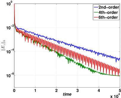
(a) Discrete modal PML (83a)–(83d)

(b) Discrete physically motivated PML (32a)–(32d)

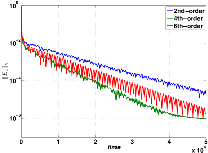
(c) Discrete split–field PML (96a)–(96d)

Fig. 3: The $l_{2}$-norm of the electric fields as a function of time

We have also performed numerous numerical experiments with different boundary parameters, $R_{x},R_{y}$ and penalty parameters $\alpha_{x},\alpha_{y},\theta_{x},\theta_{y}$. Unfortunately, because of space, we can not report all of them here. It is particularly important to note that applying the penalty $\alpha_{x}=\alpha_{y}=\theta_{x}=\theta_{y}=1$ to the discrete modal PML (82a)–(82d), with $\theta=0$, yields unstable solutions. Numerical growth was also observed when the stable boundary treatment used in (83a)–(83d) was applied to the physically motivated PML (27a)–(27d) without decreasing the time step further. This indicates that each PML model must be treated individually. A stable and efficient numerical boundary treatment for a particular PML model may not necessarily yield stable and efficient numerical scheme for another PML modeling the same physical phenomena. Of course, when the underlying physical model changes, the corresponding PML model will also change. We will also expect different stable numerical boundary treatments.

In the next section, we will verify the stability and accuracy of the PML in an electromagnetic waveguide.

6.1 Electromagnetic waveguides

Here, we will focus on the discrete PML (83a)–(83d). The results obtained for the discrete PMLs, (32a)–(32d) and (96a)–(96d), are analogous, and will not be presented. Consider the rectangular semi–infinite electromagnetic waveguide $-2\leq x<\infty$, $-1\leq y\leq 1$. At the upper wall, $y=1,$ of the waveguide, the boundary condition is a magnetic source $H_{x}(x,1,t)=F(x,1,t)$, where

$$F(x,y,t)=\exp(-\pi^{2}(f_{0}t-1)^{2})g(x,y),$$ (105)

and

$$g(x,y)=\exp\left(-\left(\left(x-1\right)^{2}+\left(y-1\right)^{2}\right)/0.01\right),\quad f_{0}=10.$$

At the lower wall, $y=-1,$ the boundary condition is homogeneous $H_{x}(x,-1,t)=0$. At the left wall, $x=-2$, we impose the characteristic boundary condition $E_{z}\left(-2,y,t\right)+H_{y}\left(-2,y,t\right)=0$. In order to perform numerical simulations, we truncate the right boundary at $x=2$ with a PML of width $\delta=0.4$. We terminate the PML at $x=2+\delta$ with the characteristic boundary condition $E_{z}(2+\delta,y,t)-H_{y}(2+\delta,y,t)=0$. Homogeneous initial conditions

$$E_{z}(x,y,0)=H_{x}(x,y,0)=H_{y}(x,y,0)=H_{x}^{*}(x,y,0)=0,$$ (106)

are used for all variables. We also use the cubic monomial damping profile

$$\begin{split}&\sigma(x)=\left\{\begin{array}[]{rl}0{}{}&\text{if}\quad|x|\leq 2,\\ d_{0}\Big{(}\frac{|x|-2}{\delta}\Big{)}^{3}&\text{if}\quad|x|\geq 2,\end{array}\right.\end{split}$$ (107)

with the damping coefficient $d_{0}=4/(2\times\delta)\log(1/(10^{-4}h)^{2})$, where the factor $10^{-4}$ is empirically determined and $h>0$ is the spatial step.

We approximate all spatial derivatives using SBP operators with interior order of accuracy 2, 4, 6. Boundary conditions are imposed weakly using penalties. As before, we discretize in time using the classical 4th order accurate Runge–Kutta method.

6.2 Numerical stability

In the first sets of experiments we investigate discrete stability. Consider SBP finite difference operators of order of accuracy 2, 4, 6, respectively. We use the spatial step $h=0.02$ and the time step $dt=0.4h$, and evolve the solutions until $t=2000$ (250 000 time steps) with $\theta=0,1$, respectively, in (83d). Note that here the domain, spatial and time steps are much smaller than the ones used in the previous sections. The snapshots of the solutions at $t=300$ are shown in figure 4, for the 4th order accurate SBP operator.

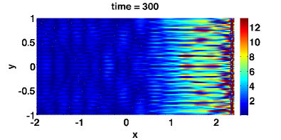
(a) $\theta=0$

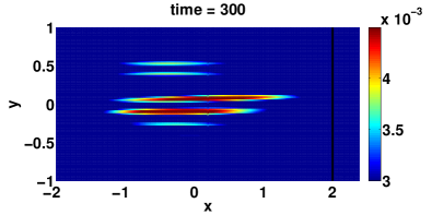
(b) $\theta=1$

Fig. 4: The snapshot of the solutions at $t=300$.

Note that initially the two solutions, using $\theta=0,1$, are similar. For the standard choice, $\theta=0$, the solution in the PML starts growing after a longtime, just before $t=200$, and spreads into the computational domain as time passes. At $t=300$, growth in the PML has already corrupted the solutions everywhere. The 2nd and 6th order accurate operators with $\theta=0$ are also unstable, but with slower growth rates. On the other hand, for $\theta=1,$ the solutions decay throughout the simulation for all SBP operators. It is important to remark that the observed growth is due to the unstable boundary treatments in the PML.

The conclusion here is that a numerical method which is stable in the absence of the PML, when $\sigma=0$, can result in an unstable scheme when, $\sigma>0$, the PML is included. It is possible though to design stable numerical methods which can be proven stable for all $\sigma\geq 0.$ Here, numerical stability for the discrete PML (83a)–(83d) was achieved by using $\theta=1$ in equation (83d) without any additional cost or difficulty.

6.3 Accuracy

Next, we evaluate the accuracy of the PML. We set $\theta=1$ and compute the solutions for various resolutions using SBP operators of interior order of accuracy 2, 4 and 6, until the final time, $t=5.$ The snapshots of the solutions at $t=1,2,3,4$ are displayed in figure 5, showing the evolution of the electric field on the boundary, the propagation and reflection of waves in the waveguide, and the absorption of waves by the PML.

The errors introduced when a PML is used in computations can be divided into two different categories: numerical reflections and the modeling error. Numerical reflections are discrete effects introduced by discretizing the PML and seen inside the computational domain. The modeling error is introduced because the layer and the magnitude of damping coefficient are finite. Numerical reflections should converge to zero as the mesh is refined. Note that the modeling error is not caused by numerical approximations, and thus is independent of the numerical method used. The modeling error is expected to decrease as the PML width or the magnitude of damping coefficient increases. For sufficiently small mesh sizes numerical reflections are infinitesimally small and the modeling error dominates the total PML error.

In order to measure numerical errors, we also computed a reference solution in a larger domain without the PML. By comparing the reference solutions to the PML solutions in the interior, measured in the maximum norm, we obtain accurate measure of total PML errors. The numerical errors at $t=5$ are displayed in table 1, and the time history of the error are shown in figure 6.

Note that the errors converge to zero exponentially. Because we have used exactly the same damping strength, $d_{0}$, for the 2nd, 4th and 6th order accurate schemes we expect to have the same modeling error independent of the accuracy of the scheme used. It is also important to note that for small mesh–sizes the modeling error dominates and the behavior of the total PML error does not depend on the order of accuracy of the scheme.

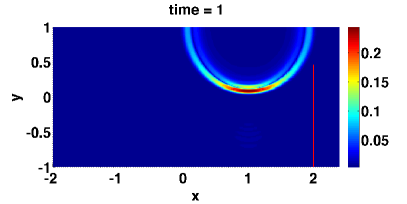
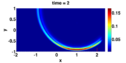
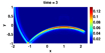
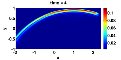
Fig. 5: Snapshots of the electric field at $t=1,2,3,4$.

	$6$th Order		$4$th Order		$2$nd Order
$h$	error	rate	error	rate	error	rate
0.04	1.08$\times 10^{-3}$	–	1.64$\times 10^{-3}$	–	2.63$\times 10^{-3}$	–
0.02	6.22$\times 10^{-6}$	7.44	5.03$\times 10^{-6}$	8.35	3.61$\times 10^{-5}$	6.19
0.01	1.93$\times 10^{-7}$	5.01	8.22$\times 10^{-8}$	5.93	7.96$\times 10^{-8}$	8.82
0.005	7.42$\times 10^{-9}$	4.70	6.67$\times 10^{-9}$	3.62	7.43$\times 10^{-9}$	3.42

Table 1: Total PML errors and the convergence of the error in a waveguide using SBP operators of interior order 2, 4, 6 for different grid resolutions.

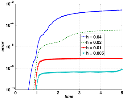
(a) Second order accuracy

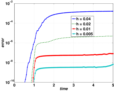
(b) Fourth order accuracy

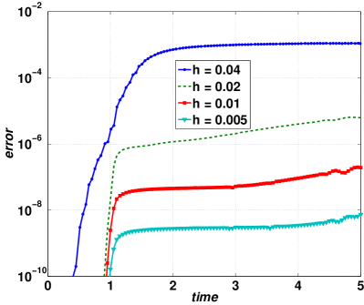
(c) Sixth order accuracy

Fig. 6: Total PML errors as a function of time using SBP operators of interior order 2, 4, 6 for different grid resolutions.

7 Summary and outlook

In this paper, we have studied the (long time) temporal energy growth associated with numerical approximations of the PML in bounded domains. Three different unsplit PML models and the classical split–field PML model are considered. We proved the stability of the constant coefficient IBVP for the PML. We also derived energy estimates for the constant coefficient IBVP in the Laplace space and for variable coefficients PML in the time domain domain. Thus, establishing well–posedness and stability of the IBVP corresponding to the PML.

We have demonstrated in theory and numerical experiments that a numerical method which is stable in the absence of the PML can become unstable when the PML is introduced. Here, the discrete stability of the PML depends only on the numerical implementation of boundary conditions; the interior approximations do not play any roles. We developed high order accurate and stable numerical approximation using SBP finite difference operators to approximate spatial derivatives and weak enforcement of boundary conditions using penalties. By constructing analogous discrete energy estimates we obtain a bound on the energy growth of the solution at any future time. Further, we showed that the corresponding constant coefficient PML problem can not support temporally growing solution. We presented numerical experiments demonstrating high order accuracy and longtime stability of the PML.

We note that a stable numerical boundary treatment for a particular PML model may not necessarily yield stable numerical solutions for another PML modeling the same physical phenomena. When the underlying physical model changes, the corresponding PML model will be different. We also expect different stable numerical boundary treatments.

Although the analysis here focuses on the Maxwell’s equations the results obtained can be straightforwardly applied to equations of acoustics.

We are currently extending the techniques described in this paper to other numerical methods such as finite element methods, spectral element methods, dG finite element/volume methods and mixed spectral-finite element methods. However, these require substantially more details and analysis. Our preliminary results are quite promising and will be reported in another paper [8]. It will be interesting to compare the results obtained from a dG method to the results obtained in this paper using high order finite difference SBP operators.

Appendix A Some useful lemmata

Introduce the complex number $z=x+iy$ and define the branch cut of $\sqrt{z}$ by

$$-\pi<\arg{\left(x+iy\right)}\leq\pi,\quad\arg{\sqrt{x+iy}}=\frac{1}{2}\arg{{\left(x+iy\right)}}.$$ (108)

The following Lemma was adapted from Lemma 6 in [37].

Lemma 11.

Let $k_{x}$ be a real number and let $s=a+ib$ be a complex number where $a>0$. Consider the relation

$$\kappa=\sqrt{s^{2}+k_{x}^{2}}.$$ (109)

There are positive real numbers $\beta_{0}\geq 1$, $0<\epsilon_{0}\leq 1$ such that $\Re{\kappa}=\beta_{0}a$, $\Im{\kappa}=\epsilon_{0}b$.

We can also prove the following lemma

Lemma 12.

Let $\sigma\geq 0$, $k_{x}$ be real numbers and let $s=a+ib$ be a complex number where $a>0$. Consider the relation

$$\widetilde{\kappa}=\sqrt{s^{2}+\left(\frac{k_{x}}{1+\frac{\sigma}{s}}\right)^{2}}.$$ (110)

There are positive real numbers $\beta_{0}\geq 1$, $0<\epsilon_{0}\leq 1$ such that

$$\Re\left(\widetilde{\kappa}\right)=\beta_{0}a+\sigma\frac{\left(\beta_{0}-\epsilon_{0}\right)b^{2}}{\left(a+\sigma\right)^{2}+b^{2}}>0.$$

Proof.

Consider

$$\begin{split}&\widetilde{\kappa}=\sqrt{s^{2}+\left(\frac{k_{x}}{1+\frac{\sigma}{s}}\right)^{2}}=\frac{s}{s+\sigma}\sqrt{\left(s+\sigma\right)^{2}+k_{x}^{2}}=\frac{a\left(a+\sigma\right)+b^{2}+ib\sigma}{\left(a+\sigma\right)^{2}+b^{2}}\left(\beta_{0}\left(a+\sigma\right)+i\epsilon_{0}b\right),\\ &\implies\Re\left(\widetilde{\kappa}\right)=\beta_{0}a+\sigma\frac{\left(\beta_{0}-\epsilon_{0}\right)b^{2}}{\left(a+\sigma\right)^{2}+b^{2}}>0.\end{split}$$

∎

Lemma 13.

Let $\sigma\geq 0$, $k_{x}$ be real numbers and let $s=a+ib$ be a complex number where $a>0$. Consider the relation

$$\kappa=\sqrt{s^{2}+k_{x}^{2}}.$$ (111)

There are positive real numbers $\beta_{0}\geq 1$, $0<\epsilon_{0}\leq 1$ such that

$$\Re\left(\left(1+\frac{\sigma}{s}\right){\kappa}\right)=\left(\beta_{0}a\left(1+\frac{\sigma a}{a^{2}+b^{2}}\right)+\epsilon_{0}\frac{\sigma b^{2}}{a^{2}+b^{2}}\right)>0,$$

Proof.

Consider

$$\begin{split}&\left(1+\frac{\sigma}{s}\right){\kappa}=\left(1+\frac{\sigma a}{a^{2}+b^{2}}-i\frac{\sigma b}{a^{2}+b^{2}}\right)\left(\beta_{0}a+i\epsilon_{0}b\right),\\ &\implies\Re\left(\left(1+\frac{\sigma}{s}\right){\kappa}\right)=\left(\beta_{0}a\left(1+\frac{\sigma a}{a^{2}+b^{2}}\right)+\epsilon_{0}\frac{\sigma b^{2}}{a^{2}+b^{2}}\right)>0.\end{split}$$

∎

Lemma 14.

Let $\sigma\geq 0$, be a nonnegative real number and $s=a+ib$ a complex number where $a>0$. Consider the relations

$$S_{x}=1+\frac{\sigma}{s}=\frac{a\left(a+\sigma\right)+b^{2}-i\sigma b}{a^{2}+b^{2}},\quad A_{0}=\frac{a^{2}+b^{2}}{\left(a\left(a+\sigma\right)+b^{2}\right)^{2}+\left(\sigma b\right)^{2}}>0.$$ (112)

We have

$$\Re{\left(\frac{1}{S_{x}}\right)} =A_{0}\left(a\left(a+\sigma\right)+b^{2}\right)>0,$$

$$\Re{\left(\frac{(sS_{x})^{*}}{S_{x}}\right)} =A_{0}\left(\left(a+\sigma\right)\left(a\left(a+\sigma\right)+b^{2}\right)+\sigma b^{2}\right)>0,$$

$$\Re\left(\frac{s^{*}}{S_{x}}\right) =A_{0}\left(a\left(a\left(a+\sigma\right)+b^{2}\right)+\sigma b^{2}\right)>0.$$

Proof.

Consider

$$\begin{split}&\frac{1}{S_{x}}=\frac{a^{2}+b^{2}}{a\left(a+\sigma\right)+b^{2}-i\sigma b}=A_{0}\left(a\left(a+\sigma\right)+b^{2}+i\sigma b\right),\\ &\implies\Re{\left(\frac{1}{S_{x}}\right)}=A_{0}\left(a\left(a+\sigma\right)+b^{2}\right)>0.\end{split}$$

Note that

$$sS_{x}=s+\sigma=a+\sigma+ib\implies\left(sS_{x}\right)^{*}=a+\sigma-ib.$$

Thus, we have

$$\frac{\left(sS_{x}\right)^{*}}{S_{x}}=A_{0}\left(a\left(a+\sigma\right)+b^{2}+i\sigma b\right)\left(a+\sigma-ib\right)\implies\Re{\left(\frac{(sS_{x})^{*}}{S_{x}}\right)}=A_{0}\left(\left(a+\sigma\right)\left(a\left(a+\sigma\right)+b^{2}\right)+\sigma b^{2}\right)>0.$$

Consider now

$$\frac{s^{*}}{S_{x}}=A_{0}\left(a\left(a+\sigma\right)+b^{2}+i\sigma b\right)\left(a-ib\right)\implies\Re{\left(\frac{s^{*}}{S_{x}}\right)}=A_{0}\left(a\left(a\left(a+\sigma\right)+b^{2}\right)+\sigma b^{2}\right)>0.$$

The proof of the lemma is complete. ∎

Appendix B Proof of Theorem 5

Multiply equation (63a) by $\partial{E_{z}}/\partial t$ and integrate over the whole domain. Integration by parts yields

$$\begin{split}&\left(\frac{\partial{E_{z}}}{\partial t},\frac{\partial^{2}{E_{z}}}{\partial t^{2}}\right)+\left(\frac{\partial{E_{z}}}{\partial t},\sigma\frac{\partial{E_{z}}}{\partial t}\right)\\ &=-\left(\frac{\partial^{2}{E_{z}}}{\partial x\partial t},\frac{\partial{E_{z}}}{\partial x}+\sigma H_{y}\right)-\left(\frac{\partial^{2}{E_{z}}}{\partial y\partial t},\frac{\partial{E_{z}}}{\partial y}+\sigma H_{x}\right)\\ &+\int_{-y_{0}}^{y_{0}}\left(\frac{\partial{E_{z}}}{\partial t}\left(\frac{\partial{E_{z}}}{\partial x}+\sigma H_{y}\right)\Big{|}_{-\left(x_{0}+\delta\right)}^{x_{0}+\delta}\right)dy+\int_{-\left(x_{0}+\delta\right)}^{x_{0}+\delta}\left(\frac{\partial{E_{z}}}{\partial t}\left(\frac{\partial{E_{z}}}{\partial y}+\sigma H_{x}\right)\Big{|}_{-y_{0}}^{y_{0}}\right)dx.\end{split}$$ (113)

Imposing the boundary conditions (64) at $y=\pm y_{0}$ and (65) at $x=\pm\left(x_{0}+\delta\right)$ , we arrive at

$$\begin{split}&\frac{1}{2}\frac{d}{dt}\left(\Big{\|}\frac{\partial{E_{z}}}{\partial t}\Big{\|}^{2}+\left(\frac{\partial{E_{z}}}{\partial x},\frac{\partial{E_{z}}}{\partial x}\right)+2\left(\frac{\partial{E_{z}}}{\partial x},\sigma H_{y}\right)+\left(\frac{\partial{E_{z}}}{\partial y},\frac{\partial{E_{z}}}{\partial y}\right)+2\left(\frac{\partial{E_{z}}}{\partial y},\sigma H_{x}\right)+\int_{\Gamma_{x}}\gamma_{y}\sigma\left(E_{z}^{2}(x,y_{0},t)+E_{z}^{2}(x,-y_{0},t)\right)dx\right)\\ &=\left(\frac{\partial{E_{z}}}{\partial x},{\sigma}\frac{\partial{H_{y}}}{\partial t}\right)+\left(\frac{\partial{E_{z}}}{\partial y},{\sigma}\frac{\partial{H_{x}}}{\partial t}\right)-\left(\frac{\partial{E_{z}}}{\partial t},\sigma\frac{\partial{E_{z}}}{\partial t}\right)-\gamma_{y}\int_{\Gamma_{x}}\left(\frac{\partial{E_{z}^{2}}}{\partial t}(x,-y_{0},t)+\frac{\partial{E_{z}^{2}}}{\partial t}(x,y_{0},t)\right)dx\\ &-\gamma_{x}\int_{\Gamma_{y}}\left(\frac{\partial{E_{z}^{2}}}{\partial t}(-x_{0}-\delta,y,t)+\frac{\partial{E_{z}^{2}}}{\partial t}(x_{0}+\delta,y,t)\right)dy.\end{split}$$ (114)

By adding

$$\frac{d}{dt}\left(\sigma H_{y},\sigma H_{y}\right)+\frac{d}{dt}\left(\sigma H_{x},\sigma H_{x}\right),$$

to both sides of equation (114) we have

$$\begin{split}&\frac{1}{2}\frac{d}{dt}\left(\Big{\|}\frac{\partial{E_{z}}}{\partial t}\Big{\|}^{2}+\Big{\|}\frac{\partial{E_{z}}}{\partial x}+\sigma H_{y}\Big{\|}^{2}+\Big{\|}\frac{\partial{E_{z}}}{\partial y}+\sigma H_{x}\Big{\|}^{2}+\Big{\|}\sigma H_{y}\Big{\|}^{2}+\Big{\|}\sigma H_{x}\Big{\|}^{2}+\gamma\sigma\|E_{z}\left(-y_{0},\mathrm{t}^{\prime}\right)\|^{2}_{\Gamma_{y}}+\gamma\sigma\|E_{z}\left(y_{0},\mathrm{t}^{\prime}\right)\|^{2}_{\Gamma_{x}}\right)\\ &=\left(\frac{\partial{E_{z}}}{\partial x},{\sigma}\frac{\partial{H_{y}}}{\partial t}\right)+\left(\frac{\partial{E_{z}}}{\partial y},{\sigma}\frac{\partial{H_{x}}}{\partial t}\right)+2\left(\frac{\partial{H_{y}}}{\partial t},\sigma^{2}{H_{y}}\right)+2\left(\frac{\partial{H_{x}}}{\partial t},\sigma^{2}{H_{x}}\right)-\left(\frac{\partial{E_{z}}}{\partial t},\sigma\frac{\partial{E_{z}}}{\partial t}\right)\\ &-\gamma_{y}\int_{\Gamma_{x}}\left(\frac{\partial{E_{z}}}{\partial t}^{2}(x,-y_{0},t)+\frac{\partial{E_{z}}}{\partial t}^{2}(x,y_{0},t)\right)dx-\gamma_{x}\int_{\Gamma_{y}}\left(\frac{\partial{E_{z}}}{\partial t}^{2}(-x_{0}-\delta,y,t)+\frac{\partial{E_{z}}}{\partial t}^{2}(x_{0}+\delta,y,t)\right)dy.\end{split}$$ (115)

By using (63b) and (63c) in the right hand side of (115), we obtain

$$\begin{split}\frac{1}{2}\frac{d}{dt}\mathcal{E}^{\left(1\right)}_{\sigma}\left(t\right)&=-\left(\frac{\partial{E_{z}}}{\partial x},{\sigma}\left(\frac{\partial{E_{z}}}{\partial x}+\sigma H_{y}\right)\right)+\left(\frac{\partial{E_{z}}}{\partial y},{\sigma}\frac{\partial{E_{z}}}{\partial y}\right)-2\left(\left(\frac{\partial{E_{z}}}{\partial x}+\sigma\left(x\right)H_{y}\right),\sigma^{2}{H_{y}}\right)+2\left(\frac{\partial{E_{z}}}{\partial y},\sigma^{2}{H_{x}}\right)\\ &-\left(\frac{\partial{E_{z}}}{\partial t},\sigma\frac{\partial{E_{z}}}{\partial t}\right),\end{split}$$ (116)

where the energy $\mathcal{E}_{\sigma}^{\left(1\right)}$ is define in (68). Note that if the boundary conditions are (66) at $y=\pm y_{0}$ and (67) at $x=\pm(x_{0}+\delta)$, from (114) we have

$$\begin{split}\frac{1}{2}\frac{d}{dt}\mathcal{E}^{\left(0\right)}_{\sigma}\left(t\right)&=-\left(\frac{\partial{E_{z}}}{\partial x},{\sigma}\left(\frac{\partial{E_{z}}}{\partial x}+\sigma H_{y}\right)\right)+\left(\frac{\partial{E_{z}}}{\partial y},{\sigma}\frac{\partial{E_{z}}}{\partial y}\right)-2\left(\left(\frac{\partial{E_{z}}}{\partial x}+\sigma\left(x\right)H_{y}\right),\sigma^{2}{H_{y}}\right)+2\left(\frac{\partial{E_{z}}}{\partial y},\sigma^{2}{H_{x}}\right)\\ &-\left(\frac{\partial{E_{z}}}{\partial t},\sigma\frac{\partial{E_{z}}}{\partial t}\right),\end{split}$$ (117)

Thus, Cauchy–Schwartz inequality and the facts $\sqrt{\mathcal{E}^{\left(1\right)}_{\sigma}\left(t\right)}\geq\|{\partial{E_{z}}}/{\partial t}\|$, $\sqrt{\mathcal{E}^{\left(1\right)}_{\sigma}\left(t\right)}\geq\|{\partial{E_{z}}}/{\partial x}+\sigma{{H_{y}}}\|$, $\sqrt{\mathcal{E}^{(1)}_{\sigma}}\geq\|\sigma{{H_{y}}}\|$, $\sqrt{\mathcal{E}^{\left(1\right)}_{\sigma}\left(t\right)}\geq\|{\partial{E_{z}}}/{\partial y}+\sigma{{H_{x}}}\|$, $\sqrt{\mathcal{E}^{\left(1\right)}_{\sigma}\left(t\right)}\geq\|\sigma{{H_{x}}}\|$ and $\sqrt{\mathcal{E}^{\left(0\right)}_{\sigma}\left(t\right)}\geq\|{\partial{E_{z}}}/{\partial t}\|$, $\sqrt{\mathcal{E}^{\left(0\right)}_{\sigma}\left(t\right)}\geq\|{\partial{E_{z}}}/{\partial x}+\sigma{{H_{y}}}\|$, $\sqrt{\mathcal{E}^{(0)}_{\sigma}}\geq\|\sigma{{H_{y}}}\|$, $\sqrt{\mathcal{E}^{\left(0\right)}_{\sigma}\left(t\right)}\geq\|{\partial{E_{z}}}/{\partial y}+\sigma{{H_{x}}}\|$, $\sqrt{\mathcal{E}^{\left(1\right)}_{\sigma}\left(t\right)}\geq\|\sigma{{H_{x}}}\|$ lead to

$$\begin{split}\frac{d}{dt}\sqrt{\mathcal{E}^{\left(1\right)}_{\sigma}\left(t\right)}\leq\sigma_{\infty}\sqrt{\mathcal{E}^{\left(1\right)}_{\sigma}\left(t\right)},\quad\frac{d}{dt}\sqrt{\mathcal{E}^{\left(0\right)}_{\sigma}\left(t\right)}\leq\sigma_{\infty}\sqrt{\mathcal{E}^{\left(0\right)}_{\sigma}\left(t\right)}.\end{split}$$ (118)

The proof of the theorem is complete. $\square$

Appendix C Proof of Theorem 7

Set $\theta=1$ in (85a) we have

$$\frac{\mathrm{d^{2}}{\mathbf{E}_{z}}}{\mathrm{dt^{2}}} =-\left(\mathrm{P}_{x}^{-1}D_{x}^{T}\otimes I_{y}\right)\left(\mathrm{P}_{x}\otimes I_{y}\right)\left(\left(D_{x}\otimes I_{y}\right)\mathbf{E}_{z}+\mathbf{\sigma}\mathbf{H}_{y}\right)-\left(I_{x}\otimes\mathrm{P}_{y}^{-1}D_{y}^{T}\right)\left(I_{x}\otimes\mathrm{P}_{y}\right)\left(\left(I_{x}\otimes D_{y}\right)\mathbf{E}_{z}+\mathbf{\sigma}\mathbf{H}_{x}\right)-\sigma\frac{\mathrm{d}{\mathbf{E}_{z}}}{\mathrm{dt}}$$

$$-\left(\mathrm{P}_{x}^{-1}\left(E_{Rx}+E_{Lx}\right)\otimes I_{y}+\left(I_{x}\otimes\mathrm{P}_{y}^{-1}\left(E_{Ry}+E_{Ly}\right)\right)\right)\frac{\mathrm{d}{\mathbf{E}_{z}}}{\mathrm{dt}}-\sigma\left(I_{x}\otimes\mathrm{P}_{y}^{-1}\left(E_{Ry}+E_{Ly}\right)\right)\mathbf{E}_{z},$$ (119a)

$$\frac{\mathrm{d}{\mathbf{H}_{y}}}{\mathrm{dt}} =-\left(D_{x}\otimes I_{y}\right)\mathbf{E}_{z}-\mathbf{\sigma}\mathbf{H}_{y},$$ (119b)

$$\frac{\mathrm{d}{\mathbf{H}_{x}}}{\mathrm{dt}} =\left(I_{x}\otimes D_{y}\right)\mathbf{E}_{z}.$$ (119c)

Multiplying equation (119a) with $\left({\mathrm{d}{\mathbf{E}_{z}}}/{\mathrm{dt}}\right)^{T}{\mathbf{P}_{xy}}$ from the left, we have

$$\begin{split}&\frac{1}{2}\frac{\mathrm{d}}{\mathrm{dt}}\Big{\langle}\frac{\mathrm{d}{\mathbf{E}_{z}}}{\mathrm{dt}},\frac{\mathrm{d}{\mathbf{E}_{z}}}{\mathrm{dt}}\Big{\rangle}_{\mathbf{P}_{xy}}+\Big{\langle}\frac{\mathrm{d}{\mathbf{E}_{z}}}{\mathrm{dt}},\left(\sigma+\left(E_{Rx}+E_{Lx}\right)\otimes\mathrm{P}_{y}+\left(\mathrm{P}_{x}\otimes\left(E_{Ry}+E_{Ly}\right)\right)\right)\frac{\mathrm{d}{\mathbf{E}_{z}}}{\mathrm{dt}}\Big{\rangle}=\\ &-\Big{\langle}\left(\left(D_{x}\otimes I_{y}\right)\mathbf{E}_{z}+\mathbf{\sigma}\mathbf{H}_{y}\right),\left(D_{x}\otimes I_{y}\right)\frac{\mathrm{d}{\mathbf{E}_{z}}}{\mathrm{dt}}\Big{\rangle}_{\mathbf{P}_{xy}}-\Big{\langle}\left(\left(I_{x}\otimes D_{y}\right)\mathbf{E}_{z}+\mathbf{\sigma}\mathbf{H}_{x}\right),\left(I_{x}\otimes D_{y}\right)\frac{\mathrm{d}{\mathbf{E}_{z}}}{\mathrm{dt}}\Big{\rangle}_{\mathbf{P}_{xy}}\\ &-\frac{\mathrm{d}{\mathbf{E}_{z}}}{\mathrm{dt}}^{T}\left(\mathrm{P}_{x}\otimes\sigma\left(E_{Ry}+E_{Ly}\right)\right)\mathbf{E}_{z}.\end{split}$$ (120)

By adding

$$\frac{d}{dt}\Big{\langle}\sigma\mathbf{H}_{y},\sigma\mathbf{H}_{y}\Big{\rangle}_{\mathbf{P}_{xy}}+\frac{d}{dt}\Big{\langle}\sigma\mathbf{H}_{x},\sigma\mathbf{H}_{x}\Big{\rangle}_{\mathbf{P}_{xy}}$$ (121)

to both sides of equation (120) we have

$$\begin{split}\frac{1}{2}\frac{d}{dt}\mathcal{E}_{h\sigma}^{\left(1\right)}\left(t\right)&=\Big{\langle}\left(D_{x}\otimes I_{y}\right)\mathbf{E}_{z},{\sigma}\frac{d{\mathbf{H}_{y}}}{dt}\Big{\rangle}_{\mathbf{P}_{xy}}+\Big{\langle}\left(I_{x}\otimes D_{y}\right)\mathbf{E}_{z},{\sigma}\frac{d{\mathbf{H}_{x}}}{dt}\Big{\rangle}_{\mathbf{P}_{xy}}+2\Big{\langle}\sigma\frac{d\mathbf{H}_{y}}{dt},\sigma\mathbf{H}_{y}\Big{\rangle}_{\mathbf{P}_{xy}}+2\Big{\langle}\sigma\frac{d\mathbf{H}_{x}}{dt},\sigma\mathbf{H}_{x}\Big{\rangle}_{\mathbf{P}_{xy}},\end{split}$$ (122)

where the energy $\mathcal{E}_{h\sigma}^{\left(1\right)}\left(t\right)$ is defined in (86). Eliminating the time derivatives on the right hand side of (122) using (85b)–(85c), we obtain

$$\begin{split}\frac{1}{2}\frac{d}{dt}\mathcal{E}_{h\sigma}^{\left(1\right)}\left(t\right)&=-\Big{\langle}\left(D_{x}\otimes I_{y}\right)\mathbf{E}_{z},{\sigma}\left(\left(D_{x}\otimes I_{y}\right)\mathbf{E}_{z}+\mathbf{\sigma}\mathbf{H}_{y}\right)\Big{\rangle}_{\mathbf{P}_{xy}}+\Big{\langle}\left(I_{x}\otimes D_{y}\right)\mathbf{E}_{z},{\sigma}\left(I_{x}\otimes D_{y}\right)\mathbf{E}_{z}\Big{\rangle}_{\mathbf{P}_{xy}}\\ &-2\Big{\langle}\sigma\left(\left(D_{x}\otimes I_{y}\right)\mathbf{E}_{z}+\mathbf{\sigma}\mathbf{H}_{y}\right),\sigma\mathbf{H}_{y}\Big{\rangle}_{\mathbf{P}_{xy}}+2\Big{\langle}\sigma\left(I_{x}\otimes D_{y}\right)\mathbf{E}_{z},\sigma\mathbf{H}_{x}\Big{\rangle}_{\mathbf{P}_{xy}}.\end{split}$$ (123)

As before, Cauchy–Schwartz inequality and the facts

$$\sqrt{\mathcal{E}_{h\sigma}^{\left(1\right)}}\geq\Big{\|}\frac{\mathrm{d}{\mathbf{E}_{z}}}{\mathrm{dt}}\Big{\|}_{\mathbf{P}_{xy}},\quad\sqrt{\mathcal{E}_{h\sigma}^{\left(1\right)}}\geq\Big{\|}\left(D_{x}\otimes I_{y}\right)\mathbf{E}_{z}+\mathbf{\sigma}\mathbf{H}_{y}\Big{\|}_{\mathbf{P}_{xy}},\quad\sqrt{\mathcal{E}_{h\sigma}^{\left(1\right)}}\geq\Big{\|}\sigma\mathbf{H}_{y}\Big{\|}_{\mathbf{P}_{xy}},$$

$$\sqrt{\mathcal{E}_{h\sigma}^{\left(1\right)}}\geq\Big{\|}\left(I_{x}\otimes D_{y}\right)\mathbf{E}_{z}+\mathbf{\sigma}\mathbf{H}_{x}\Big{\|}_{\mathbf{P}_{xy}},\quad\sqrt{\mathcal{E}_{h\sigma}^{\left(1\right)}}\geq\Big{\|}\sigma\mathbf{H}_{x}\Big{\|}_{\mathbf{P}_{xy}},$$

lead to

$$\begin{split}\frac{d}{dt}\sqrt{\mathcal{E}_{h\sigma}^{\left(1\right)}}\leq\sigma_{\infty}\sqrt{\mathcal{E}_{h\sigma}^{\left(1\right)}}.\end{split}$$ (124)

$\hfill\square$

References

• [1] S. Abarbanel, D. Gottlieb, On the construction and analysis of absorbing layers in CEM, Appl. Numer. Math., 27 (1998), 331–340.
• [2] S. Abarbanel, H. Qasimov, S. Tsynkov, Long-time performance of unsplit PMLs with explicit second order schemes, J. Sci. Comput., 41 (2009), 1–12.
• [3] S. Abarbanel, D. Gottlieb, J. S. Hesthaven, Long Time Behaviour of the Perfectly matched layer equations in computational electromagnetics, J. Sci. Comput., 17 (2002), 1–4.
• [4] S. Abarbanel and D. Gottlieb, A mathematical analysis of the PML method, J. Comput. Phys., 134 (1997), 357–363.
• [5] S. Abarbanel and A. Chertock, Strict stability of high-order compact implicit finite-difference schemes: The role of boundary conditions for for hyperbolic PDEs, I, J. Comput. Phys. 158, 1–25 (2000).
• [6] S. Abarbanel, A. Chertock and A. Yefet, Strict stability of high-order compact implicit finite-difference schemes: The role of boundary conditions for for hyperbolic PDEs, II, J. Comput. Phys. 160, 67–87 (2000).
• [7] E. Abenius, F, Edelvik and C. Johansson, Waveguide truncation using UPML in the finite-element time-domain method, Tech. report, Department of Information Technology, Uppsala University, ISSN 1404–3203; 2005–06, (2005).
• [8] T. G. Amler, K. Duru and I. Hoteit, Stable dG finite element/volume schemes for the perfectly matched layer for Maxwell’s equation, in preparation, (2014)
• [9] D. Appelö, T. Hagstrom, G. Kreiss, Perfectly matched layer for hyperbolic systems: general formulation, well-posedness and stability, SIAM J. Appl. Math., 67 (2006), 1–23.
• [10] E. Bécache, S. Fauqueux, P. Joly, Stability of perfectly matched layers, group velocities and anisotropic waves, J. Comput. Phys., 188 (2003), 399–433.
• [11] E. Bécache, P. G. Petropoulos, and S. D. Gedney, On the long-time behaviour of unsplit perfectly matched layers, IEEE Trans. on Antennas and Propag., 52 (2004), 1335–1342.
• [12] E. Bécache and P. Joly, On the analysis of Bérenger’s perfectly matched layers for Maxwell’s equations, Math. Mod. and Num. Analys., 36 (2002), 87–119.
• [13] J.-P. Bérenger, Numerical reflection from FDTD-PMLs: A comparison of the split PML with the unsplit and CFS PMLs, IEEE Trans on Antennas and Propag., 50 (2003), 258–265.
• [14] J.-P. Bérenger, A perfectly matched layer for the absorption of electromagnetic waves, J. Comput. Phys., (114) 1994, 185–200.
• [15] M. H. Carpenter, D. Gottlieb, S. Abarbanel, Time-stable boundary conditions for finite-difference schemes solving hyperbolic systems: methodology and application to high-order compact schemes, J. Comput., Phys., 111 (1994), 220–236.
• [16] W. Chew and W. Weedon, A 3-D perfectly matched medium from modified maxwell’s equations with stretched coordinates, Micro. Opt. Tech. Lett., 7 (1994), 599–604.
• [17] K. Duru, A perfectly matched layer for the time–dependent wave equation in heterogeneous and layered media, J. Comput. Phys., 257: 757-781, (2014).
• [18] K. Duru, G. Kreiss, Boundary waves and the stability of perfectly matched layer I, In Proceedings of Num. and Math. Aspects of Waves (2013).
• [19] K. Duru, G. Kreiss, Numerical interaction of boundary waves with perfectly matched layers in two space dimensional elastic waveguides, Wave Motion, DOI: 10.1016/j.wavemoti.2013.11.002 (2013).
• [20] K. Duru, G. Kreiss, A Well-posed and discretely stable perfectly matched layer for elastic wave equations in second order formulation, Commun. Comput. Phys., 11 (2012), 1643–1672.
• [21] K. Duru, G. Kreiss, Efficient and stable perfectly matched layer for CEM, DOI: http://dx.doi.org/10.1016/j.apnum.2013.09.005 (2013), Appl. Num. Maths.
• [22] K. Duru, G. Kreiss, On the accuracy and stability of the perfectly matched layers in transient waveguides, J. of Sc. Comput., DOI: 10.1007/s10915-012-9594-7, (2012).
• [23] D. Funaro and D. Gottlieb, A new method of imposing boundary conditions in pseudospeetral approximations of hyperbolic equations, Math. Comp., 51 (1988), 599–613.
• [24] G. J. Gassner, A skew-symmetric discontinuous Galerkin spectral element discretization and its relation to SBP-SAT finite difference methods, SIAM J. Sci. Comput., 35 (2013), A1233–A1253.
• [25] S. D. Gedney, An anisotropic perfectly matched layer absorbing media for the truncation of FDTD latices, IEEE Trans. on Antennas and Propag., 44 (1996), 1630–1639.
• [26] B. Gustafsson, High order difference methods for time dependent PDE, Springer–Verlag, Berlin Heidelberg, 2008.
• [27] B. Gustafsson, On the implementation of boundary conditions for method of lines, BIT Numer Math 38 (1998), 293–314.
• [28] K. O. Friedrichs, Symmetric hyperbolic linear differential equations, Comm. Pure Appl. Math., 7 (1954 ), 345–392.
• [29] K. O. Friedrichs, Symmetric positive linear differential equations, Comm. Pure Appl. Math., 11 (1958), 333–410.
• [30] K. O. Friedrichs and P. D. Lax, On symmetrizable differential operators, In Proc. Symposia in Pure Math., Amer. Math. Soc., Providence, R.I., volume 10 (1967).
• [31] T. Hagstrom, New results on absorbing layers and radiation boundary conditions, Topics in Comput. Wave Propag., Lect. Notes Comput. Sci. Eng. 31 (2003), 1–42.
• [32] L. Halpern, S. Petit-Bergez, J. Rauch, The analysis of matched layers, Conflu. Math. 3(2), 159–236 (2011).
• [33] J. Hesthaven and T. Warburton Nodal Discontinuous Galerkin Methods: Algorithms, Analysis, and Applications, Springer (2008).
• [34] J-M. Jin, W. C. Chew, Combining PML and ABC for the finite-element analysis of scattering problems, Microwave and Optical Technology Letters 12 (1996), 192–197.
• [35] K. Kormann, M. Kronbichler and B. Müller, Derivation of Strictly Stable High Order Difference Approximations for Variable-Coefficient PDE, J. Sci Comput, DOI: 10.1007/s10915-011-9479-1 (2012)
• [36] G. Kreiss, K. Duru, Discrete stability of perfectly matched layers for anisotropic wave equations in first and second order formulation, BIT Numer Math (2013), DOI: 10.1007/s10543-013-0426-4.
• [37] H.–O. Kreiss, and N.A. Petersson, Boundary estimates for the elastic wave equations in almost incompressible materials, SIAM J. Num. Anal. 50, pp. 1556-1580, DOI: 10.1137/110832847 (2012).
• [38] H–O. Kreiss, J. Lorenz, Initial-boundary value problems and the Navier-Stokes equations, first ed., Academic Press, Boston, 1989.
• [39] H.–O. Kreiss, Initial boundary value problems for hyperbolic systems, Comm. Pure Appl. Math., 23 (1970), 277–298.
• [40] M. Kuzuoglu, R. Mittra, Frequency dependence of the constitutive parameters of causal perfectly matched anisotropic absorbers, IEEE Microwave and Guided Wave Letters, 6 (1996), 447–449.
• [41] J.-L. Lions, J. Métral, O. Vacus, Well-posed absorbing layer for hyperbolic problems, Numer. Math. (2002) 92: 535–562.
• [42] Y. Y. Lu, Minimizing the discrete reflectivity of perfectly matched layers, IEEE Photonic Tech. Lett., 18 (2006), 487–489.
• [43] K. Mattsson, Boundary procedures for summation–by–parts operators, J. Sc. Comput., 18 (2003), 133–153.
• [44] M. Motamed, H–O. Kreiss, Hyperbolic initial boundary value problems which are not boundary stable, Numerical Analysis, School of Computer Science and Communication, KTH, Stockholm, Sweden (2008).
• [45] J. Nordström, Error bounded schemes for time-dependent hyperbolic problems, SIAM J. Sci. Comput., 30 (2008), 46–59.
• [46] H. Qasimov, S. Tsynkov, Lacunae based stabilization of PMLs, J. Comput. Phys., 227 (2008), 7322–7345.
• [47] B. Sjögreen, N. A. Petersson, Perfectly matched layer for Maxwell’s equation in second order formulation, J. Comput. Phys., 209 (2005), 19–46.
• [48] B. Strand, Summation by parts for finite difference approximations for d/dx, J. Comput., Phys. 110 (1994) 47–67.
• [49] M. Svärd and J. Nordström, Review of summation-by-parts schemes for initial-boundary-value problems, J. Comput., Phys., 268 (2014) 17–38.
• [50] A. Taflove, Advances in Computational Electrodynamics, The Finite-Difference Time-Domain Artec House Inc. (1998).
• [51] E. Turkel and A. Yefet, Absorbing PML boundary layers for wave–like equations, Appl. Num. Maths 27 (1998), 533–557.
• [52] K. S. Yee, Numerical solution of initial boundary value problems involving Maxwell’s equations in isotropic media, IEEE Trans. Antennas Propag., 14 (1966), 302–307.