Distributed linear programming
with event-triggered communication

Abstract

We consider a network of agents whose objective is for the aggregate of their states to converge to a solution of a linear program in standard form. Each agent has limited information about the problem data and can communicate with other agents at discrete time instants of their choosing. Our main contribution is the synthesis of a distributed dynamics and a set of state-based rules, termed triggers, that individual agents use to determine when to opportunistically broadcast their state to neighboring agents to ensure asymptotic convergence to a solution of the linear program. Our technical approach to the algorithm design and analysis overcomes a number of challenges, including establishing convergence in the absence of a common smooth Lyapunov function, ensuring that the triggers are detectable by agents using only local information, accounting for asynchronism in the state broadcasts, and ruling out various causes of arbitrarily fast state broadcasting. Various simulations illustrate our results.

1 Introduction

The global objective of many multi-agent systems can be formulated as an optimization problem where the individual agents’ states are the decision variables. Due to the inherent networked structure of these problems, much research has been devoted to developing local dynamics for each agent that guarantee that the aggregate of their states converge to a solution of the optimization problem. From an analysis viewpoint, the availability of powerful concepts and tools from stability analysis makes continuous-time coordination algorithms appealing. However, their implementation requires the continuous flow of information among agents. On the other hand, discrete-time algorithms are amenable to real-time implementation, but the selection of the stepsizes to guarantee convergence has to take into account worst-case situations, leading to an inefficient use of the network resources. In this paper, we seek to combine the advantages of both approaches by designing a distributed algorithmic solution to linear programming in standard form that combines continuous-time computation by individual agents with opportunistic event-triggered communication among neighbors. Our focus on linear programming is motivated by its importance in mathematical optimization and its pervasiveness in multi-agent scenarios, with applications to task assignment, network flow, optimal control, and energy storage, among others.

Literature review. The present work has connections with three main areas: distributed optimization, event-triggered control, and switched and hybrid systems. Distributed convex optimization problems have many applications to networked systems, see e.g., [2, 20, 24], and this has motivated the development of a growing body of work that includes dual-decomposition [22, 27], the alternating direction method of multipliers [26], subgradient projection algorithms [14, 19, 28], auction algorithms [1], and saddle-point dynamics [6, 7]. The works [4, 21] propose algorithms specifically designed for distributed linear programming. In [4], the goal is for agents to agree on the global solution. In [21], instead, the goal is for the aggregate of agents’ states to converge to a solution. All the algorithms mentioned above are implemented in either continuous or discrete time, the latter with time-dependent stepsizes that are independent of the network state. Instead, event-triggered control seeks to opportunistically adapt the execution to the network state by trading computation and decision-making for less communication, sensing or actuation effort while guaranteeing a desired level of performance, see e.g., [11, 25, 18]. In this approach to real-time implementation, a key design objective, besides asymptotic convergence, is to ensure the lack of an infinite number of updates in any finite time interval of the resulting event-triggered strategy. A few works [24, 15] have explored the design of distributed event-triggered optimization algorithms for multi-agent systems. A major difference between event-triggered stabilization and optimization is that in the former the equilibrium is known a priori, whereas in the latter the determination of the equilibrium point is the objective itself. Finally, our work is related to the literature on switched and hybrid systems [16, 12, 9] where discrete and continuous dynamical components coexist. To the authors’ knowledge, this work is the first to consider event-triggered implementations of state-dependent switched dynamical systems. A unique challenge that must be overcome in this scenario is the fact that the use of outdated state information may cause the system to miss a mode switch, and this in turn may affect the overall stability and performance.

Statement of contributions. The main contribution of the paper is the design of a provably correct distributed dynamics which, together with a set of distributed criteria to trigger state broadcasts among neighbors, enable a group of agents to collectively solve linear programs in standard form. Our starting point is the introduction of a novel distributed continuous-time dynamics for linear programming based on an exact quadratic regularization and the characterization of its solutions as saddle points of an augmented Lagrangian function. This distributed dynamics is discontinuous in the agents’ state because of the inequality constraints in the original linear program. Our approach to synthesize strategies that rely only on discrete-time communication proceeds by having agents implement the distributed continuous-time dynamics using a sample-and-hold value of their neighbors’ state. The key challenge is then to identify suitable criteria to opportunistically determine when agents should share information with their neighbors in order to guarantee asymptotic convergence and persistency of the executions. Because of the technical complexity involved in solving this challenge, we structure our discussion in two steps, dealing with the design first of centralized criteria and then of distributed ones.

Under our centralized event-triggered communication scheme, agents use global knowledge of the network to determine when to synchronously broadcast their state. The characterization of the convergence properties of the centralized implementation is challenging because the original continuous-time dynamics is discontinuous in the agents’ state and the fact that its final convergence value (being the solution of the optimization problem) is not known a priori, which further complicates the identification of a common smooth Lyapunov function. Nevertheless, using concepts and tools from switched and hybrid systems, we are able to overcome these obstacles by introducing a discontinuous Lyapunov function and examining its evolution during time intervals where state broadcasts do not occur

We build on our centralized design to synthesize a distributed event-triggered communication law under which agents use local information to determine when to broadcast their individual state. Our strategy to accomplish this is to investigate to what extent the centralized triggers can be implemented in a distributed way and modify them when necessary. In doing so, we face the additional difficulty posed by the fact that the mode switches associated to the discontinuity of the original dynamics are not locally detectable by individual agents. To address this challenge, we bound the evolution of the Lyapunov function under mode mismatch and, based on this understanding, design the distributed triggers so that any potential increase of the Lyapunov function due to the mismatch is compensated by the decrease in its value before the mismatch took place. Moreover, the distributed character of the agent triggers leads to asynchronous state broadcasts, which poses an additional challenge for both design and analysis. Our main result establishes the asymptotic convergence of the distributed implementation and identifies sufficient conditions for executions to be persistently flowing (that is, state broadcasts are separated by a uniform time infinitely often). We show that the asynchronous state broadcasts cannot be the cause of non-persistently flowing executions and we conjecture that all executions are in fact persistently flowing. As a byproduct of using a hybrid systems modeling framework in our technical approach, we are also able to guarantee that the global asymptotic stability of the proposed distributed algorithm is robust to small perturbations. Finally, simulations illustrate our results.

Organization. Section 2 introduces preliminary notions. Section 3 presents the problem statement and network model. Section 4 introduces the continuous-time dynamics on which we base our event-triggered design. Sections 5 and 6 present, respectively, centralized and distributed event-triggered mechanisms for communication and their convergence analysis. Section 7 provides simulation results in a multi-agent assignment problem and Section 8 gathers our conclusions and ideas for future work.

2 Preliminaries

This section introduces the notation and some notions from hybrid systems and optimization employed throughout the paper.

2.1 Notation

We let $\mathbb{R}$ and $\mathbb{N}$ denote the set of real and nonnegative integer numbers, respectively. For a vector $x\in\mathbb{R}^{d}$, $x\geq 0$ means that every component of $x$ is non-negative. For $x\in\mathbb{R}^{d}$, $\|x\|_{2}$ and $\|x\|_{\infty}$ denote its Euclidean and $\infty$-norm, respectively. For a matrix $A\in\mathbb{R}^{d_{1}\times d_{2}}$, its $i^{\rm th}$ row is $a_{i}$, its $(i,j)$-element is $a_{i,j}$, and its spectral radius is $\rho(A)$. Given sets $S_{1},S_{2}\subseteq\mathbb{R}^{d}$, we let $S_{1}\setminus S_{2}$ denote the elements that are in $S_{1}$ but not in $S_{2}$. We use $\operatorname{int}(S)$ to denote the set of interior points of the set $S\subseteq\mathbb{R}^{d}$. A function $f:X\rightarrow\mathbb{R}$ is locally Lipschitz at $x\in X\subset\mathbb{R}^{d}$ if there exists some neighborhood $\mathcal{U}$ of $x$ and constant $K_{x}\geq 0$ such that for all $x_{1},x_{2}\in\mathcal{U}$, it holds that $|f(x_{1})-f(x_{2})|\leq K_{x}\|x_{1}-x_{2}\|_{2}$. We say that $f$ is locally Lipschitz on $X$ if it is locally Lipschitz at $x$ for all $x\in X$. The domain of $f$ is denoted $\operatorname{dom}(f)$. The function $f$ is convex if for all $x_{1},x_{2}\in X$ and all $\lambda\in[0,1]$, it holds that $f(\lambda x_{1}+(1-\lambda)x_{2})\leq\lambda x_{1}+(1-\lambda)x_{2}$. Also, $f$ is concave if $-f$ is convex. The generalized gradient of $f$ at $\hat{x}\in X$ is defined as

$$\partial f(\hat{x}):=\operatorname{co}\bigg{\{}\lim_{i\rightarrow\infty}\nabla f(x_{i}):x_{i}\rightarrow x,x_{i}\notin S\cup\Omega_{f}\bigg{\}},$$

where $\operatorname{co}$ denotes the convex hull, $S$ is a set of measure zero, and $\Omega_{f}\subset\mathbb{R}^{d}$ is the set of points where $f$ is not differentiable. If $f$ is locally Lipschitz, its generalized gradient at any point in $X$ is non-empty. If $g:X\times Y\rightarrow\mathbb{R}$, then $\partial_{x}g(x,y)$ (resp. $\partial_{y}g(x,y)$) is the generalized gradient of the map $x\mapsto g(x,y)$ (resp. $y\mapsto g(x,y)$). For $c\in\mathbb{R}$, we denote by $f^{-1}(\leq c)=\{x\in X\;|\;f(x)\leq c\}$ the $c$-sublevel set of $f$. Given $V:\mathbb{R}^{d}\rightarrow\mathbb{R}$ and $f:\mathbb{R}^{d}\rightarrow\mathbb{R}^{d}$, the Lie derivative of $V$ along $f$ at $x$ is

(1) $$\mathcal{L}_{f}V(x):=\lim_{\alpha\rightarrow 0}\frac{V(x+\alpha f(x))-V(x)}{\alpha}.$$

We say that $\mathcal{L}_{f}V(x)$ exists when the limit in (1) exist. If $V$ is differentiable, then $\mathcal{L}_{f}V(x)=\nabla V(x)^{T}F(x)$ for $x\in\mathbb{R}^{d}$.

2.2 Hybrid systems

These basic notions on hybrid systems follow closely the exposition found in [9]. A hybrid (or cyber-physical) system is a dynamical system whose state may evolve according to (i) a differential equation $\dot{x}=f(x)$ when its state is in some subset, $C$, of the state-space and (ii) a difference equation $x^{+}=g(x)$ when its state is in some other subset, $D$, of the state-space. Thus, we may represent a hybrid system by the tuple $H=(f,g,C,D)$ where $f:\mathbb{R}^{d}\rightarrow\mathbb{R}^{d}$ (resp. $g:\mathbb{R}^{d}\rightarrow\mathbb{R}^{d}$) is called the flow map (resp. jump map) and $C\subseteq\mathbb{R}^{d}$ (resp. $D\subseteq\mathbb{R}^{d}$) is called the flow set (resp. jump set). Formally speaking, the evolution of the states of $H$ are governed by the following equations

(2a) $$\dot{x} =f(x),\quad x\in C,$$

(2b) $$x^{+} =g(x),\quad x\in D.$$

A compact hybrid time domain is a subset of $\mathbb{R}_{\geq 0}\times\mathbb{N}$ of the form

$$E=\cup_{j=0}^{J-1}([t_{j},t_{j+1}],j),$$

for some finite sequence of times $0=t_{0}\leq t_{1}\leq\dots\leq t_{J}$. It is a hybrid time domain if for all $(T,J)\in E$, $E\cap([0,T]\times\{0,\dots,J\})$ is a compact hybrid time domain. A function $\psi$ is a solution to the hybrid system (2) if

1. for all $j\in\mathbb{N}$ such that $I^{j}:=\{t:(t,j)\in\operatorname{dom}(\psi)\}$ has non-empty interior

   $$\psi(t,j) \in C,\quad \forall t\in\operatorname{int}(I^{j}),$$

   $$\dot{\psi}(t,j) =f(\psi(t,j)),\quad \text{for almost all }t\in I^{j}.$$

2. for all $(t,j)\in\operatorname{dom}(\psi)$ such that $(t,j+1)\in\operatorname{dom}(\psi)$

   $$\psi(t,j) \in D,$$

   $$\psi(t,j+1) =g(\psi(t,j)).$$

In (i) above, we say that $\psi$ is flowing and in (ii) we say that $\psi$ is jumping. We call $\psi$ persistently flowing if it is eventually continuous or if there exists a uniform time constant $\tau_{P}$ whereby $\psi$ flows for $\tau_{P}$ seconds infinitely often. Formally speaking, $\psi$ is persistently flowing if

1. $([t_{J},\infty),J)\subset\operatorname{dom}(\psi)$ for some $J\in\mathbb{N}$, or

2. there exists $\tau_{P}>0$ and an increasing sequence $\{j_{k}\}_{k=0}^{\infty}\subset\mathbb{N}$ such that $([t_{j_{k}},t_{j_{k}}+\tau_{P}],j_{k})\subset\operatorname{dom}(\psi)$ for each $k\in\mathbb{N}$.

2.3 Quadratic optimization

Here we introduce some basic definitions and results regarding mathematical optimization. A detailed exposition on these topics can be found in [3]. First, a quadratic optimization problem can be denoted by

(3a) $$\min \quad c^{T}x+\frac{1}{2}x^{T}\mathcal{E}x$$

(3b) s.t. $$\quad Ax=b,\quad x\geq 0,$$

where for $n,m\in\mathbb{N}$, $c,x\in\mathbb{R}^{n}$, $0\preceq\mathcal{E}=\mathcal{E}^{T}\in\mathbb{R}^{n\times n}$, $b\in\mathbb{R}^{m}$, and $A\in\mathbb{R}^{m\times n}$. We call (3) the primal problem and its associated dual is defined as

$$\max_{z}q(z),$$

where $q:\mathbb{R}^{m}\rightarrow\mathbb{R}$ is given by

$$q(z):=\min_{x}\bigg{\{}-\frac{1}{2}x^{T}\mathcal{E}x-b^{T}z:c+\mathcal{E}x+A^{T}z\geq 0\bigg{\}}.$$

The solutions to the primal and the dual are related through the so-called Karush-Kuhn-Tucker (KKT) conditions. A point $(x_{*},z_{*})\in\mathbb{R}^{n}\times\mathbb{R}^{m}$ satisfies the KKT conditions for (3) if

$$c+\mathcal{E}x_{*}+A^{T}z_{*}\geq 0,\quad Ax_{*}=b,\quad x_{*}\geq 0,$$

$$(c+\mathcal{E}x_{*}+A^{T}z_{*})^{T}x_{*}=0.$$

When the primal is feasible with a finite optimal value,

1. a point $(x_{*},z_{*})$ satisfies the KKT conditions for (3) if and only if $x_{*}$ (resp. $z_{*}$) is a solution to the primal (resp. the dual)

2. the optimal value of the primal is the optimal value of the dual.

3 Problem statement and network model

This section introduces the problem of interest. Our main objective is to develop a distributed algorithm for multi-agent systems that is able to solve general linear programs and takes into account the discrete nature of inter-agent communication. Given $c\in\mathbb{R}^{n}$, $b\in\mathbb{R}^{m}$, and $A\in\mathbb{R}^{m\times n}$, a linear program in standard form on $\mathbb{R}^{n}$ is defined by

(4a) $$\min \quad c^{T}x$$

(4b) s.t. $$\quad Ax=b,\quad x\geq 0.$$

Note that this is a special case of the quadratic program (3), where $\mathcal{E}=0$. We assume that (4) is feasible, with a finite optimal value, and denote by $\mathcal{X}\subseteq\mathbb{R}^{n}$ the set of solutions. Without loss of generality, we assume that

$$\text{{\bf SA \#1:}}\quad\rho(A^{T}A)\leq 1.$$

We do this for ease of presentation, as this assumption simplifies the exposition of the technical treatment. Two reasons justify the generality of SA #1: the results are easily extensible to the case $\rho(A^{T}A)>1$ and Remark 6 later presents a $O(m)$ distributed algorithm that a multi-agent network can run to ensure the assumption holds.

We next describe the model for the multi-agent network. Consider a collection of agents with unique identifiers $i\in\{1,\dots,n\}$. The state of agent $i$ is $x_{i}\in\mathbb{R}$. Each agent $i$ knows $c_{i}$ and the non-zero elements of any row $a_{\ell}$ of $A$ where $a_{\ell,i}\not=0$ (and the associated $b_{\ell}$). In addition, if $x_{i}$ and $x_{j}$ appear in a common constraint, then $i$ and $j$ have the ability to communicate with each other at discrete instants of time of their choosing. We assume communication happens instantaneously and denote by $\hat{x}_{i}$ the last state transmitted by agent $i$ to its neighboring agents. Our objective is then to design a distributed algorithm that specifies how agents should update their own states with the information they possess and when they should broadcast it to neighboring agents with the ultimate goal of making the aggregate of the agents’ states $x=(x_{1},\dots,x_{n})$ converge to a solution of (4). To solve this problem, we take an approach based on continuous-time computation with discrete-time communication. Formally, we formulate our approach using the notion of hybrid system described in Section 2.2 as follows.

Problem 1.

(Distributed linear programming with event-triggered communication). Design a hybrid system that, for each $i\in\{1,\dots,n\}$, takes the form,

(5a) $$\dot{x}_{i} =g_{i}(\hat{x}),\quad (x,\hat{x})\notin\mathcal{T}_{i}$$ if ,

(5b) $$\hat{x}_{i}^{+} =x_{i},\quad (x,\hat{x})\in\mathcal{T}_{i}$$ if ,

where $g_{i}:\mathbb{R}^{n}\rightarrow\mathbb{R}$ is agent $i$’s flow map and $\mathcal{T}_{i}\subseteq\mathbb{R}^{n}\times\mathbb{R}^{n}$ is agent $i$’s trigger set, which determines when $i$ should broadcast its state, such that

1. $g_{i}$ is computable by agent $i$ and the inclusion $(x,\hat{x})\in\mathcal{T}_{i}$ is detectable by agent $i$ using local information and communication, and

2. the aggregate of the agents’ states converge to a solution of (4).

The interpretation of Problem 1 is as follows. Equation (5a) models the fact that agent $i\in\{1,\dots,n\}$ uses the last broadcast states from neighboring agents and itself to compute the continuous-time flow $g_{i}$ governing the evolution of its state. In-between two consecutive broadcasts of agent $i$ (i.e., while flowing), there is no dynamics for its last broadcast state $\hat{x}_{i}$. Formally, $\dot{\hat{x}}_{i}=0$ if $(x,\hat{x})\notin\mathcal{T}_{i}$. For this reason, the state evolution is quite easy to compute since it changes according to a constant rate during continuous flow. Our use of the term “continuous-time flow” is motivated by the fact that we model the event-triggered design in the hybrid system framework. Moreover, viewing the dynamics (5a) as a continuous-time flow will aid our analysis in subsequent sections. Equation (5b) models the broadcast procedure. The condition $(x,\hat{x})\in\mathcal{T}_{i}$ is a state-based trigger used by agent $i$ to determine when to broadcast its current state $x_{i}$ to its neighbors. Since communication is instantaneous, $x_{i}^{+}=x_{i}$ if $(x,\hat{x})\in\mathcal{T}_{i}$. The dynamical coupling between different agents is through the broadcast states in $\hat{x}$ only. Note that an agent cannot pre-determine the time of its next state broadcast because it cannot predict if or when it will receive a broadcast from a neighbor. For this reason, we call the strategy outlined in Problem 1 event-triggered as opposed to self-triggered.

When we do not specify the continuous-time dynamics of $\hat{x}_{i}$ the reader should interpret this to mean that $\dot{\hat{x}}_{i}=0$ when $(x,\hat{x})\notin\mathcal{T}_{i}$. Likewise, $x_{i}^{+}=x_{i}$ when $(x,\hat{x})\in\mathcal{T}_{i}$. This convention holds throughout the paper.

4 Continuous-time computation and communication

In this section we introduce a distributed continuous-time algorithm that requires continuous communication to solve general linear programs in standard form. We build on this design in the forthcoming sections to provide an algorithmic solution to Problem 1 that only employs communication at discrete time instants.

We follow a design methodology similar to the one we employed in our previous work [21]. The reason for the different dynamics proposed here has to do with its amenability to event-triggered optimization and will become clearer in Section 5.

4.1 Solutions of linear program formulated as saddle points

The general approach we use for designing the continuous-time dynamics is to define an augmented Lagrangian function based on a regularization of the linear program and then derive the natural saddle-point dynamics for that function. More specifically, consider the following quadratic regularization of (4),

(6a) $$\min \quad\gamma c^{T}x+\frac{1}{2}x^{T}x$$

(6b) s.t. $$\quad Ax=b,\quad x\geq 0.$$

where $\gamma\geq 0$. We use the regularization rather than the original formulation (4) itself because, as we discuss later in Remark 10, the resulting saddle-point dynamics is amenable to event-triggered implementation. The following result reveals that this regularization is exact for suitable values of $\gamma$. The result is a modification of [17, Theorem 1] for linear programs in standard form,, rather than in inequality form.

Lemma 2.

(Exact regularization). There exists $\gamma_{\min}>0$ such that, for $\gamma\geq\gamma_{\min}$, the solution to the regularization (6) is a solution to the linear program (4).

Proof.

We use the fact that a point $x_{*}\in\mathbb{R}^{n}$ (resp. $z_{*}\in\mathbb{R}^{m}$) is a solution to (4) (resp. the dual of (4)) if and only if it satisfies the KKT conditions for (4),

(7) $$c+A^{T}z_{*}\geq 0,\quad Ax_{*}=b,\quad x_{*}\geq 0,\quad(c+A^{T}z_{*})^{T}x_{*}=0.$$

We also consider the optimization problem

(8a) $$\min \quad\frac{1}{2}x^{T}x$$

(8b) s.t. $$\quad Ax=b,\quad c^{T}x=p,\quad x\geq 0,$$

where $p$ is the optimal value of (4). Note that the solution to the above problem is a solution to (4) by construction of the constraints. Likewise, $(\bar{x},\bar{z},\bar{w})\in\mathbb{R}^{n}\times\mathbb{R}^{m}\times\mathbb{R}$ are primal-dual solutions to (8) if and only if they satisfy the KKT conditions for (8)

(9) $$\bar{x}+A^{T}\bar{z}+c\bar{w}\geq 0,\quad A\bar{x}=b,\quad c^{T}\bar{x}=p,\quad\bar{x}\geq 0,\quad(\bar{x}+A^{T}\bar{z}+c\bar{w})^{T}\bar{x}=0.$$

Since $\bar{x}$ is a solution to (4), without loss of generality, we suppose that $x_{*}=\bar{x}$. We consider the cases when (i) $\bar{w}=0$, (ii) $\bar{w}>0$, and (iii) $\bar{w}<0$. In case (i), combining (7) and (9), one can obtain for any $\gamma\geq 0$,

$$\gamma c+x_{*}+A^{T}(\gamma z_{*}+\bar{z})\geq 0,\quad Ax_{*}=b,\quad x_{*}\geq 0,\quad(\gamma c+x_{*}+A^{T}(\gamma z_{*}+\bar{z}))^{T}x_{*}=0.$$

The above conditions reveal that $(x_{*},\gamma z_{*}+\bar{z})$ satisfy the KKT conditions for (6). Thus, $x_{*}$ (which is a solution to (4)) is the solution to (6) and this would complete the proof. Next, consider case (ii). If $\gamma=\gamma_{\min}:=\bar{w}>0$, the conditions (9) can be manipulated to give

$$\gamma c+x_{*}+A^{T}\bar{z}\geq 0,\quad Ax_{*}=b,\quad x_{*}\geq 0,\quad(\gamma c+x_{*}+A^{T}\bar{z})^{T}x_{*}=0.$$

This means that $(x_{*},\bar{z})$ satisfy the KKT conditions for (6). Thus, $x_{*}$ (which is a solution to (4)) is the solution to (6) and this would complete the proof. Now, for any $\gamma\geq\gamma_{\min}$, there exists an $\eta\geq 0$ such that $\gamma=\gamma_{\min}+\eta=\bar{w}+\eta$. Combining (7) and (9), one can obtain

$$\gamma c+x_{*}+A^{T}(\eta z_{*}+\bar{z})\geq 0,\quad Ax_{*}=b,\quad x_{*}\geq 0$$

$$(\gamma c+x_{*}+A^{T}(\eta z_{*}+\bar{z})^{T}x_{*}=0.$$

This means that $(x_{*},\eta z_{*}+\bar{z})$ satisfy the KKT conditions for (6). Thus, $x_{*}$ (which is a solution to (4)) is the solution to (6) and this would complete the proof. Case (iii) can be considered analogously to case (ii) with $\gamma_{\min}:=-\bar{w}$. This completes the proof. ∎

The actual value of $\gamma_{\min}$ in Lemma 2 is somewhat generic in the following sense: if one replaces $c$ in (6) by $\bar{\gamma}c$ for some $\bar{\gamma}>0$, then the regularization is exact for $\gamma\geq\frac{\gamma_{\min}}{\bar{\gamma}}$. Therefore, to ease notation, we make the following standing assumption,

$$\text{{\bf SA \#2:}}\quad\gamma_{\min}\leq 1.$$

This justifies our focus on the case $\gamma=1$. Our next result establishes a correspondence between the solution of (6) and the saddle points of an associated augmented Lagrangian function.

Lemma 3.

(Solutions of (6) as saddle points). For $K\geq 0$, consider the augmented Lagrangian function $L^{K}:\mathbb{R}^{n}\times\mathbb{R}^{m}\rightarrow\mathbb{R}$ associated to the optimization problem (6) with $\gamma=1$,

$$L^{K}(x,z) =c^{T}x+\frac{1}{2}x^{T}x+\frac{1}{2}(Ax-b)^{T}(Ax-b)+z^{T}(Ax-b)+K\mathbbm{1}^{T}\max\{0,-x\}.$$

Then, $L^{K}$ is convex in $x$ and concave in $z$. Let $x_{*}\in\mathbb{R}^{n}$ (resp. $z_{*}\in\mathbb{R}^{m}$) be the solution to (6) (resp. a solution to the dual of (6)). Then, for $K>\|c+x_{*}+A^{T}z_{*}\|_{\infty}$, the following holds,

1. $(x_{*},z_{*})$ is a saddle point of $L^{K}$,

2. if $(\bar{x},\bar{z})$ is a saddle point of $L^{K}$, then $\bar{x}=x_{*}$ is the solution of (6).

Proof.

For any $x\in\mathbb{R}^{n}$,

$$L^{K}(x,z_{*}) =c^{T}x+\frac{1}{2}x^{T}x+\frac{1}{2}(Ax-b)^{T}(Ax-b)+z_{*}^{T}(Ax-b)+K\mathbbm{1}^{T}\max\{0,-x\}$$

$$\geq c^{T}x+\frac{1}{2}x^{T}x+z_{*}^{T}(Ax-b)+\|c+x_{*}+A^{T}z_{*}\|_{\infty}x$$

$$\geq c^{T}x+\frac{1}{2}x^{T}x+z_{*}^{T}(Ax-b)-(c+x_{*}+A^{T}z_{*})^{T}x$$

$$\geq c^{T}x+\frac{1}{2}x^{T}x+z_{*}^{T}A(x-x_{*})-(c+x_{*}+A^{T}z_{*})^{T}(x-x_{*})$$

$$\geq c^{T}x+\frac{1}{2}x^{T}x-(c+x_{*})^{T}(x-x_{*})$$

$$\geq c^{T}x_{*}+\frac{1}{2}(x-x_{*})^{T}(x-x_{*})+\frac{1}{2}x_{*}^{T}x_{*}$$

(10) $$\geq c^{T}x_{*}+\frac{1}{2}x_{*}^{T}x_{*}=L^{K}(x_{*},z_{*}).$$

For any $z$, it is easy to see that $L^{K}(x_{*},z)=L^{K}(x_{*},z_{*})$. Thus $(x_{*},z_{*})$ is a saddle point of $L^{K}$.

Let us now prove (ii). As a necessary condition for $(\bar{x},\bar{z})$ to be a saddle point of $L^{K}$, it must be that $\partial_{z}L^{K}(\bar{x},\bar{z})=A\bar{x}-b=0$ as well as $L^{K}(x_{*},\bar{x})\geq L^{K}(\bar{x},\bar{z})$ which means that

(11) $$c^{T}x_{*}+\frac{1}{2}x_{*}^{T}x_{*}\geq c^{T}\bar{x}+\frac{1}{2}\bar{x}^{T}\bar{x}+K\mathbbm{1}^{T}\max\{0,-\bar{x}\}.$$

If $\bar{x}\geq 0$ then $c^{T}x_{*}+\frac{1}{2}x_{*}^{T}x_{*}\geq c^{T}\bar{x}+\frac{1}{2}\bar{x}^{T}\bar{x}$ and thus $\bar{x}$ would be a solution to (6). Consider then that $\bar{x}\not\geq 0$. Then,

$$c^{T}\bar{x}+\frac{1}{2}\bar{x}^{T}\bar{x} =c^{T}x_{*}+\frac{1}{2}x_{*}^{T}x_{*}+(c+x_{*})^{T}(\bar{x}-x_{*})+\frac{1}{2}(\bar{x}-x_{*})^{T}(\bar{x}-x_{*})$$

$$\geq c^{T}x_{*}+\frac{1}{2}x_{*}^{T}x_{*}+(c+x_{*})^{T}(\bar{x}-x_{*})$$

$$\geq c^{T}x_{*}+\frac{1}{2}x_{*}^{T}x_{*}-z_{*}^{T}A(\bar{x}-x_{*})+(c+x_{*}+A^{T}z_{*})^{T}(\bar{x}-x_{*})$$

$$\geq c^{T}x_{*}+\frac{1}{2}x_{*}^{T}x_{*}-z_{*}^{T}(A\bar{x}-b)+(c+x_{*}+A^{T}z_{*})^{T}\bar{x}$$

$$\geq c^{T}x_{*}+\frac{1}{2}x_{*}^{T}x_{*}-\|c+x_{*}+A^{T}z_{*}\|_{\infty}\max\{0,-\bar{x}\}$$

$$>c^{T}x_{*}+\frac{1}{2}x_{*}^{T}x_{*}-K\mathbbm{1}^{T}\max\{0,-\bar{x}\},$$

contradicting (11). Thus, $\bar{x}\geq 0$ and must be the solution to (6). ∎

4.2 Distributed continuous-time dynamics

Given the results in Lemmas 2 and 3, a sensible strategy to find a solution of (4) is to employ the saddle-point dynamics associated to the augmented Lagrangian function $L^{K}$. Formally, we set

(12a) $$\dot{x} \in-\partial_{x}L^{K}(x,z),$$

(12b) $$\dot{z} =\partial_{z}L^{K}(x,z).$$

This dynamics is well-defined since $L^{K}$ is a locally Lipschitz function. For an appropriate choice of the parameter $K$, one can establish the asymptotic convergence of trajectories of the saddle-point dynamics to a point in the set $\mathcal{X}\times\mathbb{R}^{m}$. However, we build the event-triggered implementation on a different dynamics that does not require precise knowledge of $K$. The following result reveals that one can characterize certain elements of the saddle-point dynamics, regardless of $K$, which will allow us to design a discontinuous dynamics later.

Lemma 4.

(Generalized gradients of the Lagrangian). Let $f:\mathbb{R}^{n}\times\mathbb{R}^{m}\rightarrow\mathbb{R}^{n}$ be defined by $f(x,z)=-(A^{T}z+c+x)-A^{T}(Ax-b)$. Given a compact set $X\times Z\subset\mathbb{R}^{n}_{\geq 0}\times\mathbb{R}^{m}$, let

$$K_{*}(X\times Z):=\max_{(x,z)\in X\times Z}\|f(x,z)\|_{\infty}.$$

Then, if $K\geq K_{*}(X\times Z)$, for each $(x,z)\in X\times Z$, $\partial_{z}L^{K}(x,z)=\{Ax-b\}$ and there exists $a\in-\partial_{x}L^{K}(x,z)\subset\mathbb{R}^{n}$ such that, for each $i\in\{1,\dots,n\}$,

$$a_{i} =\begin{cases}f_{i}(x,z),\hskip 40.4029pt\text{{\rm if} $x_{i}>0$},\\ \max\{0,f_{i}(x,z)\},\;\text{{\rm if} $x_{i}=0$}.\end{cases}$$

Proof.

Let $(x,z)\in\mathbb{R}^{n}\times\mathbb{R}^{m}$. It is straightforward to see that $\partial_{z}L^{K}(x,z)=\{Ax-b\}$ for any $K$. Next, note that for any $a\in-\partial_{x}L^{K}(x,z)$, we have

(13) $$-a-(A^{T}z+c+x)-A^{T}(Ax-b)\in K\partial\max\{0,-x\},$$

or, equivalently, $-a+f(x,z)\in K\partial\max\{0,-x\}$. For any $i\in\{1,\dots,n\}$ such that $x_{i}>0$, the corresponding set in the right-hand side of (13) is the singleton $0$ and therefore $a_{i}=f_{i}(x,z)$. On the other hand, if $x_{i}=0$, then

$$-a_{i}+f_{i}(x,z)\in[-K,0].$$

If $f_{i}(x,z)\geq 0$, the choice $a_{i}=f_{i}(x,z)$ satisfies the equation. Conversely, if $f_{i}(x,z)<0$, then $a_{i}=0$ satisfies the equation for all $K\geq K_{*}(X\times Z)$ by definition of $K_{*}(X\times Z)$. This completes the proof. ∎

As suggested previously, the above result enables us to propose an alternative continuous-time (discontinuous) dynamics to solve (4) that does not require knowledge of $K$. Specifically, Lemma 4 implies that, on a compact set, the trajectories of the dynamics

(14a) $$\dot{x}_{i} =\begin{cases}f_{i}(x,z),&\text{if $x_{i}>0$},\\ \max\{0,f_{i}(x,z)\},&\text{if $x_{i}=0$},\end{cases}$$

(14b) $$\dot{z} =Ax-b,$$

with $i\in\{1,\dots,n\}$, are trajectories of (12). That is, any bounded trajectory of (14) is also a trajectory of (12). As a consequence, the convergence properties of the saddle-point dynamics are also inherited by (14) and this is the dynamics that we design an event-triggered implementation for in the next sections. Besides the standard considerations in designing an event-triggered implementation (such as ensuring convergence and preventing arbitrarily fast broadcasting), we face several unique challenges including the fact that the equilibria of (14) are not known a priori as well as having to account for the switched nature of the dynamics.

We conclude this section by discussing the distributed implementation of (14) based on the network model of Section 3.

Remark 5.

(Distributed implementation via virtual agents). Note that the dynamics (14) possess auxiliary variables $z\in\mathbb{R}^{m}$ corresponding to the Lagrange multipliers of the optimization problem. For the purpose of analysis, we consider $m$ virtual agents with identifiers $\{n+1,\dots,n+m\}$, where virtual agent $n+\ell$ updates the state $z_{\ell}\in\mathbb{R}$ and has knowledge of the data $a_{\ell}\in\mathbb{R}^{n}$ and $b_{\ell}\in\mathbb{R}$. It is important to observe that, in an actual implementation, the state and dynamics of virtual agent $n+\ell$ can be stored and implemented by any of the real agents with knowledge of $a_{\ell}$ and $b_{\ell}$. For each $\ell\in\{1,\dots,m\}$, the set of agents

$$\{i\in\{1,\dots,n\}:a_{\ell,i}\not=0\}\cup\{n+\ell\},$$

can communicate their state information to each other. In words, if $x_{i}$ and $x_{j}$ appear in constraint $\ell$, then agents $i,j$, and $n+\ell$ can communicate with each other. The neighbor set of $i$, denoted $\mathcal{N}_{i}$, is the set of all agents that $i$ can communicate with. The set of real (resp. virtual) neighbors of $i$ is $\mathcal{N}_{i}^{x}:=\mathcal{N}_{i}\cap\{1,\dots,n\}$ (resp. $\mathcal{N}_{i}^{z}:=\mathcal{N}_{i}\cap\{n+1,\dots,n+m\}$). Under these assumptions, it is straightforward to verify that agent $i\in\{1,\dots,n\}$ can compute $f_{i}(x,z)$ using local information and can thus implement (14a). Likewise, a virtual agent $n+\ell\in\{n+1,\dots,n+m\}$ can compute and implement its corresponding dynamics $\dot{z}_{\ell}=a_{\ell}^{T}x-b_{\ell}$ in (14b). The network structure described here is quite natural for many real-world network optimization problems that can be formulated as linear programs. $\bullet$

Remark 6.

(Distributed algorithm to enforce SA #1). Given the model described in Remark 5, we explain briefly here how agents can implement a simple pre-processing algorithm based on $\max$-consensus to ensure that $\rho(A^{T}A)\leq 1$. For each row $a_{\ell}$ of the matrix $A$, the virtual agent $n+\ell$ can compute the $\ell^{\operatorname{th}}$ row of $A^{T}A$. Then, this agent stores the following estimate of the spectral radius,

$$\hat{\rho}_{n+\ell}=(A^{T}A)_{(\ell,\ell)}+\sum_{\begin{subarray}{c}i\in\{1,\dots,n\}\setminus\{\ell\}\end{subarray}}|(A^{T}A)_{(\ell,i)}|.$$

The virtual agents use these estimates as an initial point in the standard $\max$-consensus algorithm [5]. In $O(m)$ steps, the $\max$-consensus converges to a point $\rho_{*}\geq\rho(A^{T}A)$, where the inequality is a consequence of the Gershgorin Circle Theorem [13, Corollary 6.1.5]. Then, each virtual agent scales its corresponding row of $A$ and entry of $b$ by $1/\rho_{*}$, and communicates this new data to its neighbors. The resulting linear program is $\min\{c^{T}x:\tilde{A}x=\tilde{b},\;x\geq 0\}$, with $\tilde{A}=A/\rho_{*}$ and $\tilde{b}=b/\rho_{*}$. Both the solutions and optimal value of the new linear program are the same as the original linear program and, by construction, $\rho(\tilde{A}^{T}\tilde{A})\leq 1$. $\bullet$

5 Algorithm design with centralized event-triggered communication

Here, we build on the discussion of Section 4 to address the main objective of the paper as outlined in Problem 1. Our starting point is the distributed continuous-time algorithm (14), which requires continuous-time communication. Our approach is divided in two steps because of the complexity of the challenges (e.g., asymptotic convergence, asynchronism, and Zeno behavior) involved in going from continuous-time to opportunistic discrete-time communication. In this section, we design a centralized event-triggered scheme that the network can use to determine in an opportunistic way when information should be updated. In the next section, we build on this development to design a distributed event-triggered communication scheme that individual agents can employ to determine when to share information with their neighbors.

The problem we solve in this section can be formally stated as follows.

Problem 7.

(Linear programming with centralized event-triggered communication). Identify a set $\mathcal{T}^{c}\subseteq\mathbb{R}^{n}_{\geq 0}\times\mathbb{R}^{m}\times\mathbb{R}^{n}_{\geq 0}\times\mathbb{R}^{m}$ such that the hybrid system that, for $i\in\{1,\dots,n\}$, takes the form,

(15a) $$\dot{x}_{i} =\begin{cases}f_{i}(\hat{x},\hat{z}),&\hat{x}_{i}>0,\\ \max\{0,f_{i}(\hat{x},\hat{z})\},&\hat{x}_{i}=0,\end{cases}$$

(15b) $$\dot{z} =A\hat{x}-b,$$

if $$(x,z,\hat{x},\hat{z})\not\in\mathcal{T}^{c}$$ and

(15c) $$(\hat{x}^{+},\hat{z}^{+})=(x,z),$$

if $(x,z,\hat{x},\hat{z})\in\mathcal{T}^{c}$, makes the aggregate $x\in\mathbb{R}^{n}$ of the real agents’ states converge to a solution of the linear program (4).

We refer to the set $\mathcal{T}^{c}$ in Problem 7 as the centralized trigger set. Note that, in this centralized formulation of the problem, we do not require individual agents, but rather the network as a whole, to be able to detect whether $(x,z,\hat{x},\hat{z})\in\mathcal{T}^{c}$. In addition, when this condition is enabled, state broadcasts among agents are performed synchronously, as described by (15c). Our strategy to design $\mathcal{T}^{c}$ is to first identify a candidate Lyapunov function and study its evolution along the trajectories of (15). We then synthesize $\mathcal{T}^{c}$ based on the requirement that our Lyapunov function decreases along the trajectories of (15) and conclude with a result showing that the desired convergence properties are attained.

Before we introduce the candidate Lyapunov function, we present an alternative representation of (15a)-(15b) that will be useful in our analysis later. Given $(\hat{x},\hat{z})\in\mathbb{R}_{\geq 0}\times\mathbb{R}^{m}$, let $\sigma(\hat{x},\hat{z})$ be the set of agents $i$ for which $\dot{x}_{i}=f_{i}(\hat{x},\hat{z})$ in (15a). Formally,

$$\sigma(\hat{x},\hat{z})=\big{\{}i\in\{1,\dots,n\}:f_{i}(\hat{x},\hat{z})\geq 0\;\text{or}\;\hat{x}_{i}>0\big{\}}.$$

Next, let $I_{\sigma(\hat{x},\hat{z})}\in\mathbb{R}^{n\times n}$ be defined by

$$(I_{\sigma(\hat{x},\hat{z})})_{i,j}=\begin{cases}0,\;\text{if $i\not=j$ or $i\notin\sigma(\hat{x},\hat{z})$},\\ 1,\;\text{otherwise.}\end{cases}$$

Note that this matrix is an identity-like matrix with a zero $(i,i)$-element if $i\notin\sigma(\hat{x},\hat{z})$. The matrix $I_{\sigma(\hat{x},\hat{z})}$ has the following properties,

$$I_{\sigma(\hat{x},\hat{z})}\succeq 0,\quad I_{\sigma(\hat{x},\hat{z})}=I_{\sigma(\hat{x},\hat{z})}^{T},\quad I_{\sigma(\hat{x},\hat{z})}^{2}=I_{\sigma(\hat{x},\hat{z})},\quad\rho(I_{\sigma(\hat{x},\hat{z})})\leq 1.$$

Then, a compact representation of (15a)-(15b) is

$$(\dot{x},\dot{z}) =F(\hat{x},\hat{z}):=(I_{\sigma(\hat{x},\hat{z})}f(\hat{x},\hat{z}),A\hat{x}-b),$$

where $F=(F_{x},F_{z}):\mathbb{R}_{\geq 0}^{n}\times\mathbb{R}^{m}\rightarrow\mathbb{R}^{n}\times\mathbb{R}^{m}$.

5.1 Candidate Lyapunov function and its evolution

Now let us define and analyze the candidate Lyapunov function that we use to design the trigger set $\mathcal{T}^{c}$. The overall Lyapunov function is the sum of $2$ separate functions $V_{1}$ and $V_{2}$, that we introduce next. To define $V_{1}:\mathbb{R}^{n}\times\mathbb{R}^{m}\rightarrow\mathbb{R}_{\geq 0}$, fix $\mathcal{K}>\|c+x_{*}+A^{T}z_{*}\|_{\infty}$ where $x_{*}$ (resp. $z_{*}$) is the solution to (6) (resp. any solution of the dual of (6)) and let $(\bar{x},\bar{z})$ be a saddle-point of $L^{\mathcal{K}}$. Then

$$V_{1}(x,z) =\frac{1}{2}(x-\bar{x})^{T}(x-\bar{x})+\frac{1}{2}(z-\bar{z})^{T}(z-\bar{z}).$$

Note that $V_{1}\geq 0$ is smooth with compact sublevel sets. Next, $V_{2}:\mathbb{R}^{n}\times\mathbb{R}^{m}\rightarrow\mathbb{R}_{\geq 0}$ is given by

$$V_{2}(x,z) =\frac{1}{2}f(x,z)^{T}I_{\sigma(x,z)}f(x,z)+\frac{1}{2}(Ax-b)^{T}(Ax-b).$$

Note that $V_{2}\geq 0$ but, due to the state-dependent matrix $I_{\sigma(x,z)}$, is only piecewise smooth. In this sense $V_{2}$ can be viewed as a collection of multiple (smooth) Lyapunov functions, each defined on a neighborhood where $\sigma$ is constant. Also, $V_{2}^{-1}(0)$ is, by definition, the set of saddle-points of $L^{\mathcal{K}}$ (cf. Lemma 4). It turns out that the negative terms in the Lie derivative of $V_{1}$ alone are insufficient to ensure that $V_{1}$ is always decreasing given any practically implementable trigger design (by practically implementable we mean a trigger design that does not demand arbitrarily fast state broadcasting). The analogous statement regarding $V_{2}$ is also true which is why we consider instead a candidate Lyapunov function $V:\mathbb{R}^{n}\times\mathbb{R}^{m}\rightarrow\mathbb{R}_{\geq 0}$ that is their sum

$$V(x,z)=(V_{1}+V_{2})(x,z).$$

The following result states an upper bound on $\mathcal{L}_{F}V$ in terms of the state errors in $x$ and $z$.

Proposition 8.

(Evolution of $V$). Let $X\times Z\subseteq\mathbb{R}_{\geq 0}^{n}\times\mathbb{R}^{m}$ be compact and suppose that $(x,z,\hat{x},\hat{z})\in X\times Z\times X\times Z$ is such that $\sigma(\hat{x},\hat{z})\subseteq\sigma(x,z)$ and

(16) $$\sigma(x,z)=\lim_{\alpha\rightarrow 0}\sigma(x+\alpha F_{x}(\hat{x},\hat{z}),z+\alpha F_{z}(\hat{x},\hat{z})).$$

Then $\mathcal{L}_{F}V(x,z)$ exists and

$$\mathcal{L}_{F}V(x,z) \leq-\frac{1}{2}f(\hat{x},\hat{z})^{T}I_{\sigma(\hat{x},\hat{z})}f(\hat{x},\hat{z})-\frac{1}{4}(A\hat{x}-b)^{T}(A\hat{x}-b)+40e_{x}^{T}e_{x}+20e_{z}^{T}e_{z}$$

(17) $$\quad+15f(x,z)^{T}I_{\sigma(x,z)\setminus\sigma(\hat{x},\hat{z})}f(x,z),$$

where $e_{x}=x-\hat{x}$ and $e_{z}=z-\hat{z}$.

Proof.

For convenience, we use the shorthand notation $p=\sigma(x,z)$ and $\hat{p}=\sigma(\hat{x},\hat{z})$. Consider first $V_{1}$, which is differentiable and thus $\mathcal{L}_{F}V_{1}(x,z)$ exists,

$$\mathcal{L}_{F}V_{1}(x,z) =(x-\bar{x})^{T}I_{\hat{p}}f(\hat{x},\hat{z})+(z-\bar{z})^{T}(A\hat{x}-b)$$

(18) $$=(\hat{x}-\bar{x})^{T}I_{\hat{p}}f(\hat{x},\hat{z})+(\hat{z}-\bar{z})^{T}(A\hat{x}-b)+e_{x}^{T}I_{\hat{p}}f(\hat{x},\hat{z})+e_{z}^{T}(A\hat{x}-b).$$

Since $X\times Z$ is compact, without loss of generality assume that $\mathcal{K}\geq K_{*}(X\times Z)$ so that $-I_{\hat{p}}f(\hat{x},\hat{z})\in\partial_{x}L^{\mathcal{K}}(\hat{x},\hat{z})$, cf. Lemma 4. This, together with the fact that $L^{\mathcal{K}}$ is convex in its first argument, implies

$$L^{\mathcal{K}}(\hat{x},\hat{z})\leq L^{\mathcal{K}}(\bar{x},\hat{z})-(\hat{x}-\bar{x})^{T}I_{\hat{p}}f(\hat{x},\hat{z}).$$

Since $L^{\mathcal{K}}$ is linear in $z$, we can write

$$L^{\mathcal{K}}(\hat{x},\hat{z})=L^{\mathcal{K}}(\hat{x},\bar{z})+(\hat{z}-\bar{z})^{T}(A\hat{x}-b).$$

Substituting these expressions into (18), we get

$$\mathcal{L}_{F}V_{1}(x,z) \leq L^{\mathcal{K}}(\bar{x},\hat{z})-L^{\mathcal{K}}(\hat{x},\bar{z})+e_{x}^{T}I_{\hat{p}}f(\hat{x},\hat{z})+e_{z}^{T}(A\hat{x}-b)$$

$$\leq c^{T}\bar{x}+\frac{1}{2}\bar{x}^{T}\bar{x}-c^{T}\hat{x}-\frac{1}{2}\sum_{i=1}^{n}\hat{x}^{T}\hat{x}-\bar{z}^{T}(A\hat{x}-b)-\mathcal{K}\mathbbm{1}^{T}\max\{0,-\hat{x}\}$$

$$\quad-\frac{1}{2}(A\hat{x}-b)^{T}(A\hat{x}-b)+e_{x}^{T}I_{\hat{p}}f(\hat{x},\hat{z})+e_{z}^{T}(A\hat{x}-b).$$

From the analysis in the proof of Lemma 3, inequality (4.1) showed that

$$c^{T}\bar{x}+\frac{1}{2}\bar{x}^{T}\bar{x}$$

$$\quad\leq c^{T}\hat{x}+\frac{1}{2}\hat{x}^{T}\hat{x}+\bar{z}^{T}(A\hat{x}-b)+\frac{1}{2}(A\hat{x}-b)^{T}(A\hat{x}-b)+\mathcal{K}\mathbbm{1}^{T}\max\{0,-\hat{x}\},$$

where we use the fact that $\bar{x}$ is also a solution to (6), cf. Lemma 3. Therefore,

$$\mathcal{L}_{F}V_{1}(x,z) \leq-\frac{1}{2}(A\hat{x}-b)^{T}(A\hat{x}-b)+e_{x}^{T}I_{\hat{p}}f(\hat{x},\hat{z})+e_{z}^{T}(A\hat{x}-b)$$

$$\leq-\frac{1}{2}(A\hat{x}-b)^{T}(A\hat{x}-b)+\frac{\kappa}{2}(A\hat{x}-b)^{T}(A\hat{x}-b)$$

(19) $$\quad+\frac{\kappa}{2}f(\hat{x},\hat{z})^{T}I_{\hat{p}}f(\hat{x},\hat{z})+\frac{1}{2\kappa}e_{x}^{T}e_{x}+\frac{1}{2\kappa}e_{z}^{T}e_{z},$$

where we have used Lemma 15. Next, let us consider $V_{2}$. We begin by showing that (16) is sufficient for $\mathcal{L}_{F}V_{2}(x,z)$ to exist. Since $\sigma$ is a discrete set of indices, for the limit in (16) to exist, there must exist an $\bar{\alpha}>0$ such that

$$\sigma(x,z)=\sigma(x+\alpha F_{x}(\hat{x},\hat{z}),z+\alpha F_{z}(\hat{x},\hat{z})),$$

for all $\alpha\in[0,\bar{\alpha}]$. This means that one can substitute $I_{\sigma(x,z)}$ for $I_{\sigma(x+\alpha F_{x}(\hat{x},\hat{z}),z+\alpha F_{z}(\hat{x},\hat{z}))}$ in the definition of the Lie derivative (1). Since $I_{\sigma(x,z)}$ is constant with respect to $\alpha$, it is straightforward to see that

$$\mathcal{L}_{F}V_{2}(x,z) =\frac{1}{2}\nabla(f(x,z)^{T}I_{p}f(x,z))^{T}F(\hat{x},\hat{z})+\frac{1}{2}\nabla((Ax-b)^{T}(Ax-b))^{T}F(\hat{x},\hat{z}).$$

Thus,

$$\mathcal{L}_{F}V_{2}(x,z) =f(x,z)^{T}I_{p}(D_{x}f(x,z)F_{x}(\hat{x},\hat{z})+D_{z}f(x,z)F_{z}(\hat{x},\hat{z}))+(Ax-b)^{T}AF_{x}(\hat{x},\hat{z})$$

$$=-f(x,z)^{T}I_{p}(A^{T}A+I)I_{\hat{p}}f(\hat{x},\hat{z})-f(x,z)^{T}I_{p}A^{T}(A\hat{x}-b)$$

(20) $$\quad+(Ax-b)^{T}AI_{\hat{p}}f(\hat{x},\hat{z}).$$

Due to the assumption that $\hat{p}\subseteq p$, we can write $I_{p}=I_{\hat{p}}+I_{p\setminus\hat{p}}$. Also, $f(x,z)$ can be written equivalently in terms of the errors $e_{x},e_{z}$ as

$$f(x,z)=f(\hat{x},\hat{z})-A^{T}e_{z}-e_{x}-A^{T}Ae_{x}.$$

Likewise, $Ax-b=A\hat{x}-b+Ae_{x}$. Substituting these quantities into (20),

$$\mathcal{L}_{F}V_{2}(x,z) =-(f(\hat{x},\hat{z})-A^{T}e_{z}-e_{x}-A^{T}Ae_{x})^{T}I_{\hat{p}}(A^{T}A+I)I_{\hat{p}}f(\hat{x},\hat{z})$$

$$\quad-f(x,z)^{T}I_{p\setminus\hat{p}}(A^{T}A+I)I_{\hat{p}}f(\hat{x},\hat{z})$$

$$\quad-(f(\hat{x},\hat{z})-A^{T}e_{z}-e_{x}-A^{T}Ae_{x})^{T}I_{\hat{p}}A^{T}(A\hat{x}-b)$$

(21) $$\quad-f(x,z)^{T}I_{p\setminus\hat{p}}A^{T}(A\hat{x}-b)+(A\hat{x}-b+Ae_{x})^{T}AI_{\hat{p}}f(\hat{x},\hat{z}).$$

We now derive upper bounds for a few terms in (21). For example,

$$e_{z}^{T}AI_{\hat{p}}A^{T}AI_{\hat{p}}f(\hat{x},\hat{z}) \leq\frac{1}{2\kappa}e_{z}^{T}e_{z}+\frac{\kappa}{2}f(\hat{x},\hat{z})^{T}I_{\hat{p}}A^{T}AI_{\hat{p}}A^{T}AI_{\hat{p}}A^{T}AI_{\hat{p}}f(\hat{x},\hat{z})$$

$$\leq\frac{1}{2\kappa}e_{z}^{T}e_{z}+\frac{\kappa}{2}f(\hat{x},\hat{z})^{T}I_{\hat{p}}f(\hat{x},\hat{z}),$$

where we have used Lemma 15 and Theorem 16 along with the facts that $\rho(A^{T}A)=\rho(AA^{T})\leq 1$ and $\rho(I_{\hat{p}})\leq 1$. Likewise,

$$e_{x}^{T}I_{\hat{p}}A^{T}AI_{\hat{p}}f(\hat{x},\hat{z}) \leq\frac{1}{2\kappa}e_{x}^{T}e_{x}+\frac{\kappa}{2}f(\hat{x},\hat{z})^{T}I_{\hat{p}}A^{T}AI_{\hat{p}}A^{T}AI_{\hat{p}}f(\hat{x},\hat{z})$$

$$\leq\frac{1}{2\kappa}e_{x}^{T}e_{x}+\frac{\kappa}{2}f(\hat{x},\hat{z})^{T}I_{\hat{p}}f(\hat{x},\hat{z}),$$

and

$$f(x,z)^{T}I_{p\setminus\hat{p}}A^{T}(A\hat{x}-b) \leq\frac{1}{2\kappa}f(x,z)^{T}I_{p\setminus\hat{p}}f(x,z)+\frac{\kappa}{2}(A\hat{x}-b)^{T}AA^{T}(A\hat{x}-b)$$

$$\leq\frac{1}{2\kappa}f(x,z)^{T}I_{p\setminus\hat{p}}f(x,z)+\frac{\kappa}{2}(A\hat{x}-b)^{T}(A\hat{x}-b).$$

Repeatedly bounding every term in (21) in an analogous way (which we omit for the sake of space and presentation) and adding the bound (19), we attain the following inequality

$$\mathcal{L}_{F}V(x,z) \leq-(1-5\kappa)f(\hat{x},\hat{z})^{T}I_{\hat{p}}f(\hat{x},\hat{z})-\frac{1}{2}(1-5\kappa)(A\hat{x}-b)^{T}(A\hat{x}-b)$$

$$\quad+\frac{3}{2\kappa}f(x,z)^{T}I_{p\setminus\hat{p}}f(x,z)+\frac{4}{\kappa}e_{x}^{T}e_{x}+\frac{2}{\kappa}e_{z}^{T}e_{z}.$$

Equation (17) follows by choosing $\kappa=\frac{1}{10}$, completing the proof. ∎

The reason why we have only considered the case $\sigma(\hat{x},\hat{z})\subseteq\sigma(x,z)$ (and not the more general case of $\sigma(\hat{x},\hat{z})\not=\sigma(x,z)$) when deriving the bound (17) in Proposition 8 is the following: our distributed trigger design later (specifically, the trigger sets $\mathcal{T}^{0}_{i}$ introduced in Section 6) ensures that $\sigma(\hat{x},\hat{z})\subseteq\sigma(x,z)$ always. For this reason, we need not know how $V$ evolves in the more general case.

5.2 Centralized trigger set design and convergence analysis

Here, we use our knowledge of the evolution of the function $V$, cf. Proposition 8, to design the centralized trigger set $\mathcal{T}^{c}$. Our approach is to incrementally design subsets of $\mathcal{T}^{c}$ and then combine them at the end to define $\mathcal{T}^{c}$. The main observation that we base our design on is the following: The first two terms in the right-hand-side of (17) are negative and thus desirable and the rest are positive. However, following a state broadcast, the positive terms become zero. This motivates our first trigger set that should belong to $\mathcal{T}^{c}$,

(22) $$\mathcal{T}^{c,e}:=\{(x,z,\hat{x},\hat{z})\in(\mathbb{R}_{\geq 0}^{n}\times\mathbb{R}^{m})^{2}:\;A\hat{x}-b\not=0\text{ or }I_{\sigma(\hat{x},\hat{z})}f(\hat{x},\hat{z})\not=0,\text{ and}\\ \frac{1}{8}(A\hat{x}-b)^{T}(A\hat{x}-b)+\frac{1}{4}f(\hat{x},\hat{z})^{T}I_{\sigma(\hat{x},\hat{z})}f(\hat{x},\hat{z})\leq 20e_{z}^{T}e_{z}+40e_{x}^{T}e_{x}\}.$$

The numbers $\tfrac{1}{8}$ and $\tfrac{1}{4}$ in the inequalities that define $\mathcal{T}^{c,e}$ are design choices that we have made to ease the presentation. Any other choice in $(0,1)$ is also possible, with the appropriate modifications in the ensuing exposition. Note that, when both $A\hat{x}-b=I_{\sigma(\hat{x},\hat{z})}f(\hat{x},\hat{z})=0$, no state broadcasts are required since the system is at a (desired) equilibrium.

Likewise, after a state broadcast, $\sigma(x,z)=\sigma(\hat{x},\hat{z})$ and $I_{\sigma(x,z)\setminus\sigma(\hat{x},\hat{z})}=0$ which means that the last term in (17) is also zero. For this reason, define

(23) $$\mathcal{T}^{c,\sigma}:=\{(x,z,\hat{x},\hat{z})\in(\mathbb{R}_{\geq 0}^{n}\times\mathbb{R}^{m})^{2}:\sigma(x,z)\not=\sigma(\hat{x},\hat{z})\},$$

which prescribes a state broadcast when the mode $\sigma$ changes.

We require one final trigger for the following reason. While the set $\mathbb{R}_{\geq 0}^{n}\times\mathbb{R}^{m}$ is invariant under the continuous-time dynamics (14), this does not hold any more in the event-triggered case because agents use outdated state information. To preserve the invariance of this set, we define

(24) $$\mathcal{T}^{c,0} :=\{(x,z,\hat{x},\hat{z})\in(\mathbb{R}_{\geq 0}^{n}\times\mathbb{R}^{m})^{2}:\exists i\in\{1,\dots,n\}\text{ s.t. }\hat{x}_{i}>0,\,x_{i}=0\}.$$

If this trigger is activated by some agent $i$’s state becoming zero, then it is easy to see from the definition of the dynamics (15a) that $\dot{x}_{i}\geq 0$ after the state broadcast and thus $x_{i}$ remains non-negative. Finally, the overall centralized trigger set is

(25) $$\mathcal{T}^{c}:=\mathcal{T}^{c,e}\cup\mathcal{T}^{c,\sigma}\cup\mathcal{T}^{c,0}.$$

The following result characterizes the convergence properties of (15) under the centralized event-triggered communication scheme specified by (25).

Theorem 9.

(Convergence of the centralized event-triggered design). If $\psi$ is a persistently flowing solution of (15) with $\mathcal{T}^{c}$ defined as in (25), then there exists a point $(x_{*},z^{\prime})\in\mathcal{X}\times\mathbb{R}^{m}$ such that,

$$\psi(t,j)\rightarrow(x_{*},z^{\prime},x_{*},z^{\prime})\quad\text{as}\quad t+j\longrightarrow\infty,\quad(t,j)\in\operatorname{dom}(\psi).$$

Proof.

Let $(t,j)\mapsto\psi(t,j)=(x(t,j),z(t,j),\hat{x}(t,j),\hat{z}(t,j))$. We begin the proof by showing that $V$ is non-increasing along $\psi$. To this end, it suffices to prove that (a) $\mathcal{L}_{F}V(x(t,j),z(t,j))\leq 0$ when $\psi$ is flowing and $\mathcal{L}_{F}V(x(t,j),z(t,j))$ exists, (b) $V(x(t,j),z(t,j))\leq\lim_{\tau\rightarrow t^{-}}V(x(t,j),z(t,j))$ when $\psi(t,j)$ is flowing but $\mathcal{L}_{F}V(x(t,j),z(t,j))$ does not exist, and (c) $V(x(t,j+1),z(t,j+1))\leq V(x(t,j),z(t,j))$ when $\psi$ is jumping.

We begin with (a) and consider $(t,j)\in\operatorname{dom}(\psi)$ for which $\psi$ is flowing. Then, the interval $I^{j}:=\{t:(t,j)\in\operatorname{dom}(\psi)\}$ has non-empty interior and $t\in\operatorname{int}(I^{j})$. This means that $\psi(t,j)\notin\mathcal{T}^{c}$ and, in particular, $\sigma(x(t,j),z(t,j))=\sigma(\hat{x}(t,j),\hat{z}(t,j))$ by construction of $\mathcal{T}^{c,\sigma}$. Also, let $X\times Z$ be a compact set such that $\psi(t,j)\in X\times Z\times X\times Z$. Therefore, the conditions of Proposition 8 are satisfied and $\mathcal{L}_{F}V(x(\tau,j),z(\tau,j))$ exists for all $\tau\in\operatorname{int}(I^{j})$. Using (17), it holds that

$$\mathcal{L}_{F}V(x(t,j),z(t,j)) \leq-\frac{1}{8}(A\hat{x}(t,j)-b)^{T}(A\hat{x}(t,j)-b)$$

$$\quad-\frac{1}{4}f(\hat{x}(t,j),\hat{z}(t,j))^{T}I_{\sigma(\hat{x}(t,j),\hat{z}(t,j))}f(\hat{x}(t,j),\hat{z}(t,j)),$$

where we have used (i) the fact that, since $\sigma(x(t,j),z(t,j))=\sigma(\hat{x}(t,j),\hat{z}(t,j))$, the last quantity in (17) is zero and (ii) the bound on $20e_{x}^{T}e_{x}+40e_{z}^{T}e_{z}$ in the definition of $\mathcal{T}^{c,e}$. Clearly, in this case, $\mathcal{L}_{F}V(x(t,j),z(t,j))\leq 0$ when $\psi(t,j)\in X\times Z\times X\times Z$.

Next, consider (b). Since $V_{1}$ is smooth, $\mathcal{L}_{F}V_{1}(x(t,j),z(t,j))$ exists, however, when $V_{2}(x(t,j),z(t,j))$ is discontinuous, $\mathcal{L}_{F}V(x(t,j),z(t,j))$ does not. This happen at any $(t,j)\in\operatorname{dom}(\psi)$ for which (i) $I^{j}$ (as defined previously) has non-empty interior and (ii) $\sigma(x(t,j),z(t,j))\not=\lim_{\tau\rightarrow t^{-}}\sigma(x(\tau,j),z(\tau,j))$ (cf. Proposition 8). Note that condition (i) ensures that the limit in condition (ii) is well-defined. For purposes of presentation, define the sets

$$\mathcal{S}_{+}:=\sigma(x(t,j),z(t,j))\setminus\text{$\textstyle\lim_{\tau\rightarrow t^{-}}$}\sigma(x(\tau,j),z(\tau,j)),$$

$$\mathcal{S}_{-}:=\text{$\textstyle\lim_{\tau\rightarrow t^{-}}$}\sigma(x(\tau,j),z(\tau,j))\setminus\sigma(x(t,j),z(t,j)).$$

Note that one of $\mathcal{S}_{+},\mathcal{S}_{-}$ may be empty. We can write

$$V_{2}(x(t,j),z(t,j))=\text{$\textstyle\lim_{\tau\rightarrow\tau^{-}}$}V_{2}(x(\tau,j),z(\tau,j))\\ +\frac{1}{2}\text{$\textstyle\sum_{i\in\mathcal{S}_{+}}$}f_{i}(x(t,j),z(t,j))^{2}-\frac{1}{2}\text{$\textstyle\sum_{i\in\mathcal{S}_{-}}$}f_{i}(x(t,j),z(t,j))^{2}.$$

For each $i\in\mathcal{S}_{+}$, it must be that $f_{i}(x(t,j),z(t,j))=0$ since $f_{i}(\hat{x}(t,j),\hat{z}(t,j))<0$ and $f,x,z$ are continuous. Moreover, the last term in the right-hand-side of the above expression is non-positive. Thus, $V_{2}(x(t,j),z(t,j))\leq\lim_{\tau\rightarrow t^{-}}V_{2}(x(\tau,j),z(\tau,j))$.

Next, when $\psi$ is jumping, as is case (c), $V(x(t,j),z(t,j))=V(x(t,j+1),z(t,j+1)$ because $(x(t,j+1),z(t,j+1))=(x(t,j),z(t,j))$ according to (15c).

To summarize, $V(x(t,j),z(t,j))$ is non-increasing when $\psi(t,j)\in X\times Z\times X\times Z$. Without loss of generality, we choose $X\times Z=V^{-1}(\leq c)$, where $c=V(x(0,0),z(0,0))$. $X\times Z$ is compact because the sublevel sets of $V_{1}$ are compact, and $X\times Z\times X\times Z$ is invariant so as not to contradict $V(x(t,j),z(t,j))$ being non-increasing on $X\times Z\times X\times Z$. Thus, $V(x(t,j),z(t,j))$ is non-increasing at all times and $\psi$ is bounded.

Now we establish the convergence property of (15). First note that, in this preliminary design, $\psi$ being persistently flowing implies also that the Lie derivative of $V$ along $F$ exists for $\tau_{P}$ time on those intervals of persistent flow. This is because $\psi$ flowing implies that $\sigma$ is constant and thus the Lie derivative of $V$ along $F$ exists (cf. (16)). There are two possible characterizations of persistently flowing $\psi$ as given in Section 2. Consider (PFi). By the boundedness of $\psi$ just established, it must be that for all $t\geq t_{J}$

$$0 =\dot{x}(t,j) =I_{\sigma(\hat{x}(t_{J},J),\hat{z}(t_{J},J))}f(\hat{x}(t_{J},J)),\hat{z}(t_{J},J)),$$

$$0 =\dot{z}(t,j) =A\hat{x}(t_{J},J)-b.$$

By Lemma 4 this means that $(\hat{x}(t_{J},J),\hat{z}(t_{J},J))$ is a saddle-point of $L^{\mathcal{K}}$ (without loss of generality, we assume that $\mathcal{K}\geq K_{*}(X\times Z)$). Applying Lemma 3 reveals that $\hat{x}(t_{J},J)\in\mathcal{X}$. Since $\hat{x}(t,j)$ is a sampled version of $x(t_{J},J)$ it is clear that $x(t_{J},J)\in\mathcal{X}$ as well, and since their dynamics are stationary in finite time, they converge to a point, completing the proof.

Consider then (PFii), the second characterization of persistently flowing. We have established that $\{V(x(t_{j_{k}},j_{k}),z(t_{j_{k}},j_{k}))\}_{k=0}^{\infty}$ is non-increasing. Since it is also bounded from below by 0, by the monotone convergence theorem there exists a $V_{*}\in[0,c]$ such that $\lim_{k\rightarrow\infty}V(x(t_{j_{k}},j_{k}),z(t_{j_{k}},j_{k}))=V_{*}$. Thus

$$V(x(t_{j_{k}},j_{k}),z(t_{j_{k}},j_{k}))-V(x(t_{j_{k+1}},j_{k+1}),z(t_{j_{k+1}},j_{k+1}))\rightarrow 0.$$

Let $\delta>0$ and consider $\kappa\in\mathbb{N}$ such that

$$V(x(t_{j_{k}},j_{k}),z(t_{j_{k}},j_{k}))-V(x(t_{j_{k+1}},j_{k+1}),z(t_{j_{k+1}},j_{k+1}))<\delta,$$

for all $k\geq\kappa$. By the bound established on $\mathcal{L}_{F}V(x(t,j_{k}),z(t,j_{k}))$, which exists for all $(t,j_{k})\in([t_{j_{k}},t_{j_{k}}+\tau_{P}),j_{k})$, it holds that,

$$V(x(t_{j_{k+1}}, j_{k+1}),z(t_{j_{k+1}},j_{k+1}))$$

$$\leq V(x(t_{j_{k}},j_{k}),z(t_{j_{k}},j_{k}))-\frac{1}{8}(A\hat{x}(t_{j_{k}},j_{k})-b)^{T}(A\hat{x}(t_{j_{k}},j_{k})-b)\tau_{P}$$

$$\quad-\frac{1}{4}f(\hat{x}(t_{j_{k}},j_{k}),\hat{z}(t_{j_{k}},j_{k}))^{T}I_{\sigma(\hat{x}(t_{j_{k}},j_{k}),\hat{z}(t_{j_{k}},j_{k}))}f(\hat{x}(t_{j_{k}},j_{k}),\hat{z}(t_{j_{k}},j_{k}))\tau_{P}.$$

Therefore, $V(x(t_{j_{k}},j_{k}),z(t_{j_{k}},j_{k}))-V(x(t_{j_{k+1}},j_{k+1}),z(t_{j_{k+1}},j_{k+1}))<\delta$ for all $k\geq\kappa$ implies that

$$f(\hat{x}(t_{j_{k}},j_{k}),\hat{z}(t_{j_{k}},j_{k}))^{T}I_{\sigma(\hat{x}(t_{j_{k}},j_{k}),\hat{z}(t_{j_{k}},j_{k}))}f(\hat{x}(t_{j_{k}},j_{k}),\hat{z}(t_{j_{k}},j_{k})) \leq 4\delta\tau_{P},$$

$$(A\hat{x}(t_{j_{k}},j_{k})-b)^{T}(A\hat{x}(t_{j_{k}},j_{k})-b) \leq 8\delta\tau_{P},$$

for all $k\geq\kappa$. Since $\tau_{P}$ is a uniform constant and $\delta>0$ can be taken arbitrarily small, we deduce

$$I_{\sigma(\hat{x}(t_{j_{k}},j_{k}),\hat{z}(t_{j_{k}},j_{k}))}f(\hat{x}(t_{j_{k}},j_{k}),\hat{z}(t_{j_{k}},j_{k}))\rightarrow 0\quad\text{and}\quad A\hat{x}(t_{j_{k}},j_{k})-b\rightarrow 0,$$

as $k\rightarrow\infty$. By Lemma 4, this means that $(\hat{x}(t_{j_{k}},j_{k}),\hat{z}(t_{j_{k}},j_{k}))$ converges to the set of saddle-points of $L^{\mathcal{K}}$. The same argument holds for $x(t_{j_{k}},j_{k})$ since $\hat{x}(t_{j_{k}},j_{k})$ is a sampled version of that state.

Finally, we establish the convergence to a point. By the Bolzano-Weierstrass Theorem, there exists a subsequence $\{j_{k_{\ell}}\}$ such that $(x(t_{j_{k_{\ell}}},j_{k_{\ell}}),z(t_{j_{k_{\ell}}},j_{k_{\ell}}))$ converges to a saddle-point $(\bar{x}^{\prime},\bar{z}^{\prime})$ of $L^{\mathcal{K}}$. Fix $\delta^{\prime}>0$ and let $\ell_{*}$ be such that

$$\|(x(t_{j_{k_{\ell}}},j_{k_{\ell}}),z(t_{j_{k_{\ell}}},j_{k_{\ell}}))-(\bar{x}^{\prime},\bar{z}^{\prime})\|_{2}<\delta^{\prime},$$

for all $\ell\geq\ell_{*}$. Consider the function $W=W_{1}+V_{2}$ where

$$W_{1}(x,z)=\frac{1}{2}(x-\bar{x}^{\prime})^{T}(x-\bar{x}^{\prime})+\frac{1}{2}(z-\bar{z}^{\prime})^{T}(z-\bar{z}^{\prime}).$$

Let $c^{\prime}=W(x(t_{j_{k_{\ell_{*}}}},j_{k_{\ell_{*}}}),z(t_{j_{k_{\ell_{*}}}},j_{k_{\ell_{*}}}))$ and $X^{\prime}\times Z^{\prime}=W^{-1}(\leq c^{\prime})$. Repeating the previous analysis, but for $W$ instead of $V$, we deduce that $X^{\prime}\times Z^{\prime}\times X^{\prime}\times Z^{\prime}$ is invariant. Consequently, $\|(x(t,j),z(t,j))-(\bar{x}^{\prime},\bar{z}^{\prime})\|_{2}<\delta^{\prime}$ for all $(t,j)\in\operatorname{dom}(\psi)$ such that $t+j\geq t_{j_{k_{\ell_{*}}}}+j_{k_{\ell_{*}}}$. Since $\delta^{\prime}>0$ is arbitrary, it holds that

$$\psi(t,j)\rightarrow(\bar{x}^{\prime},\bar{z}^{\prime},\bar{x}^{\prime},\bar{z}^{\prime})\quad\text{as}\quad t+j\longrightarrow\infty,\quad(t,j)\in\operatorname{dom}(\psi).$$

Since $(\bar{x}^{\prime},\bar{z}^{\prime})$ is a saddle-point of $L^{\mathcal{K}}$ and, without loss of generality $\mathcal{K}\geq K_{*}(X\times Z)$, applying Lemma 3 reveals that $\bar{x}^{\prime}\in\mathcal{X}$, which completes the proof. ∎

Remark 10.

(Motivation for quadratic regularization of linear program). Here we revisit the claim made in Section 4 that using the saddle-point dynamics derived for the original linear program (4) would not be amenable to an event-triggered implementation. If we were to follow the same design methodology for such dynamics, we would find that the bound on the Lie derivative of $V$ would resemble (17), but without the non-positive term $-f(\hat{x},\hat{z})^{T}I_{\sigma(\hat{x},\hat{z})}f(\hat{x},\hat{z})$. Following the same methodology to identify the trigger set, one would then use the trigger

$$\frac{1}{8}(A\hat{x}-b)^{T}(A\hat{x}-b)\leq 20e_{z}^{T}e_{z}+40e_{x}^{T}e_{x},$$

to define $\mathcal{T}^{c,e}$ and ensure that the function $V$ does not increase. However, this trigger may easily result in continuous-time communication: consider a scenario where $A\hat{x}-b=0$, but the state $x$ is still evolving. Then the trigger would require continuous-time broadcasting of $x$ to ensure that $e_{x}$ remains zero. $\bullet$

6 Algorithm design with distributed event-triggered communication

In this section, we provide a distributed solution to Problem 1, e.g., a coordination algorithm to solve linear programs requiring only communication at discrete instants of time triggered by criteria that agents can evaluate with local information. Our strategy to accomplish this is to investigate to what extent the centralized triggers identified in Section 5.2 can be implemented in a distributed way. In turn, making these triggers distributed poses the additional challenge of dealing with the asynchronism in the state broadcasts across different agents, which raises the possibility of non-persistency in the solutions. We deal with both issues in our forthcoming discussion and establish the convergence of our distributed design.

6.1 Distributed trigger set design

Here, we design distributed triggers that individual agents can evaluate with the local information available to them to guarantee the monotonically decreasing evolution of the candidate Lyapunov function $V$. Our design methodology builds on the centralized trigger sets $\mathcal{T}^{c,e}$, $\mathcal{T}^{c,\sigma}$, and $\mathcal{T}^{c,0}$ of Section 5.2. As a technical detail, the distributed algorithm that results from this section has an extended state which, for ease of notation, we denote by

$$\xi=(x,z,s,q,r,\hat{x},\hat{z})\subseteq\Xi:=\mathbb{R}^{n}_{\geq 0}\times\mathbb{R}^{m}\times\mathbb{R}^{n}_{\geq 0}\times\{0,1\}^{(n+m)\times n}\times\mathbb{R}^{n+m}\times\mathbb{R}^{n}_{\geq 0}\times\mathbb{R}^{m}.$$

The meaning and dynamics of states $s,q,$ and $r$ will be revealed as they become necessary in our development.

We start by showing how the inequality that defines whether the network state belongs to the set $\mathcal{T}^{c,e}$ in (22) can be distributed across the group of agents. Given $\mu_{1},\dots,\mu_{n+m}>0$, consider the following trigger set for each agent,

$$\mathcal{T}^{e}_{i}:=\begin{cases}\{\xi\in\Xi:f_{i}(\hat{x},\hat{z})\not=0\text{ and }(e_{x})_{i}^{2}\geq\mu_{i}f_{i}(\hat{x},\hat{z})^{2}\},\;&\text{{\rm if $i\leq n$,}}\\ \{\xi\in\Xi:a_{i-n}^{T}\hat{x}-b_{i-n}\not=0\text{ and }(e_{z})_{i-n}^{2}\geq\mu_{i}(a_{i-n}^{T}\hat{x}-b_{i-n})^{2}\},\!&\text{{\rm if $i\geq n+1$.}}\end{cases}$$

If each $\mu_{i}\leq\tfrac{1}{160}$ and $(x,z,\hat{x},\hat{z})$ is such that the inequalities defining each $\mathcal{T}^{e}_{i}$ do not hold, then it is clear that $(x,z,\hat{x},\hat{z})\notin\mathcal{T}^{c,e}$. To ensure convergence of the resulting algorithm, we later characterize the specific ranges for the design parameters $\{\mu_{i}\}_{i=1}^{n+m}$.

Next, we show how the inclusion of the network state in the triggered set $\mathcal{T}^{c,0}$ defined in (24) can be easily evaluated by individual agents with partial information. In fact, for each $i\in\{1,\dots,n\}$, define the set

$$\mathcal{T}^{0}_{i}:=\{\xi\in\Xi:\hat{x}_{i}>0\text{ but }x_{i}=0\}.$$

Clearly, $(x,z,\hat{x},\hat{z})\in\mathcal{T}^{c,0}$ if and only if there is $i\in\{1,\dots,n\}$ such that $\xi\in\mathcal{T}^{0}_{i}$.

The triggered set $\mathcal{T}^{c,\sigma}$ defined in (23) presents a greater challenge from a distributed computation viewpoint. The problem is that, in the absence of fully up-to-date information from its neighbors, an agent will fail to detect the mode switches that characterize the definition of this set. The specific scenario we refer to is the following: assume agent $i\in\{1,\dots,n\}$ has $x_{i}=0$ and the information available to it confirms that its state should remain constant, i.e., with $f_{i}(\hat{x},\hat{z})<0$. If the condition $f_{i}(x,z)\geq 0$ becomes true as the network state evolves, this fact is undetectable by $i$ with its outdated information. In such a case, $i\notin\sigma(\hat{x},\hat{z})$ but $i\in\sigma(x,z)$, meaning that the equality $\sigma(x,z)=\sigma(\hat{x},\hat{z})$ defining the trigger set $\mathcal{T}^{c,\sigma}$ would not be not enforced. To deal with this issue, we first need to understand the effect that a mismatch in the modes has on the evolution of the candidate Lyapunov function $V$. We address this in the following result.

Proposition 11.

(Bound on evolution of candidate Lyapunov function under mode mismatch). Suppose that $(\hat{x},\hat{z})\in\mathbb{R}_{\geq 0}^{n}\times\mathbb{R}^{m}$ is such that $i\notin\sigma(\hat{x},\hat{z})$ for some $i\in\{1,\dots,n\}$ and let $t\mapsto(x(t),z(t))$ be the solution to

$$(\dot{x},\dot{z}) =F(\hat{x},\hat{z}),$$

starting from $(\hat{x},\hat{z})$. Let $T>0$ be the minimum time such that $i\in\sigma(x(T),z(T))$. Then, for any $\nu>0$, and all $t$ such that $t-T<\frac{\nu}{2\sqrt{2}}$, the following holds,

$$f_{i}(x(t),z(t))^{2}\leq\nu^{2}f(\hat{x},\hat{z})^{T}I_{\sigma(\hat{x},\hat{z})\cap\mathcal{N}^{x}_{i}}f(\hat{x},\hat{z})+\nu^{2}(A\hat{x}-b)^{T}I_{\mathcal{N}^{z}_{i}}(A\hat{x}-b).$$

Proof.

We use the shorthand notation $\hat{p}=\sigma(\hat{x},\hat{z})$ and $p(t)=\sigma(x(t),z(t))$. Since $i\notin\hat{p}$, it must be that $\hat{x}_{i}=0$ and $f_{i}(\hat{x},\hat{z})<0$. Moreover, if $i\in p(T)$, it must be, by continuity of $t\mapsto(x(t),z(t))$ and $(x,z)\mapsto f(x,z)$, that $f_{i}(x(T),z(T))=0$. Let us compute the Taylor expansion of $t\mapsto f_{i}(x(t),z(t))$ using $t=T$ as the initial point. For technical reasons, we actually consider the equivalent mapping $t\mapsto I_{\{i\}}f(x(t),z(t))$ instead,

$$I_{\{i\}}f(x(t),z(t)) =I_{\{i\}}f(x(T),z(T))+D_{x}I_{\{i\}}f(x(T),z(T))^{T}F_{x}(\hat{x},\hat{z})(t-T)$$

$$\quad+D_{z}I_{\{i\}}f(x(T),z(T))^{T}F_{z}(\hat{x},\hat{z})(t-T)$$

$$=I_{\{i\}}(A^{T}A+I)I_{\hat{p}}f(\hat{x},\hat{z})(t-T)+I_{\{i\}}A^{T}(A\hat{x}-b)(t-T),$$

where the equality holds because the higher order terms are zero. Thus,

$$f(x(t),z(t))^{T}I_{\{i\}}f(x(t),z(t)) =f(\hat{x},\hat{z})^{T}I_{\hat{p}}(A^{T}A+I)I_{\{i\}}(A^{T}A+I)I_{\hat{p}}f(\hat{x},\hat{z})(t-T)^{2}$$

$$\quad+2f(\hat{x},\hat{z})^{T}I_{\hat{p}}(A^{T}A+I)I_{\{i\}}A^{T}(A\hat{x}-b)(t-T)^{2}$$

$$\quad+(A\hat{x}-b)^{T}AI_{\{i\}}A^{T}(A\hat{x}-b)(t-T)^{2}.$$

Using Lemma 15 with $\kappa=\frac{1}{2}$ and exploiting the consistency between the matrix $A$ and the neighbors of $i$, we obtain

$$f(x(t) ,z(t))^{T}I_{\{i\}}f(x(t),z(t))$$

$$\leq 2f(\hat{x},\hat{z})^{T}I_{\hat{p}}(A^{T}A+I)I_{\{i\}}(A^{T}A+I)I_{\hat{p}}f(\hat{x},\hat{z})(t-T)^{2}$$

$$\quad+2(A\hat{x}-b)^{T}AI_{\{i\}}A^{T}(A\hat{x}-b)(t-T)^{2}$$

$$\leq 2f(\hat{x},\hat{z})^{T}I_{\hat{p}\cap\mathcal{N}^{x}_{i}}(A^{T}A+I)^{2}I_{\hat{p}\cap\mathcal{N}^{x}_{i}}f(\hat{x},\hat{z})(t-T)^{2}$$

$$\quad+2(A\hat{x}-b)^{T}I_{\mathcal{N}^{z}_{i}}AA^{T}I_{\mathcal{N}^{z}_{i}}(A\hat{x}-b)(t-T)^{2}$$

$$\leq 8f(\hat{x},\hat{z})^{T}I_{\hat{p}\cap\mathcal{N}^{x}_{i}}f(\hat{x},\hat{z})(t-T)^{2}+2(A\hat{x}-b)^{T}I_{\mathcal{N}^{z}_{i}}(A\hat{x}-b)(t-T)^{2}$$

$$\leq 8(t-T)^{2}(f(\hat{x},\hat{z})^{T}I_{\hat{p}\cap\mathcal{N}^{x}_{i}}f(\hat{x},\hat{z})+(A\hat{x}-b)^{T}I_{\mathcal{N}^{z}_{i}}(A\hat{x}-b)).$$

Using the bound $t-T\leq\frac{\nu}{2\sqrt{2}}$ in the statement of the result completes the proof. ∎

The importance of Proposition 11 comes from the following observation: given the upper bound on the evolution of the candidate Lyapunov function $V$ obtained in Proposition 8, one can appropriately choose the value of $\nu$ so that the negative terms in (17) can compensate for the presence of the last term due to a mode mismatch of finite time length. This observation motivates the introduction of the following trigger sets, which cause neighbors to send synchronized broadcasts periodically to an agent if its state remains at zero. First, if an agent $i$’s state is zero and it has not received a synchronized broadcast from its neighbors for $\tau_{i}$ time (here, $\tau_{i}>0$ is a design parameter), it triggers a broadcast to notify its neighbors that it requires new states. This behavior is captured by the trigger set

$$\mathcal{T}_{i}^{\operatorname{request}}:=\begin{cases}\{\xi\in\Xi:x_{i}=0\text{ and }s_{i}\geq\tau_{i}\},\;&\text{{\rm if $i\leq n$,}}\\ \emptyset,\;&\text{{\rm if $i\geq n+1$.}}\end{cases}$$

where we use the state $s_{i}$ to denote the time since $i$ has last sent a broadcast. On the receiving end, if $i$ receives a broadcast request from a neighbor $j$, then it should also broadcast immediately,

$$\mathcal{T}_{i}^{\operatorname{send}}:=\{\xi\in\Xi:\exists j\in\mathcal{N}_{i}^{x}\text{ s.t. }q_{i,j}=1\}.$$

where $q_{i,j}\in\{0,1\}$ is a state with $q_{i,j}=1$ indicating that $j$ has requested a broadcast from $i$.

Our last component of the distributed trigger design addresses the problem posed by the asynchronism in state broadcasts. In fact, given that agents determine autonomously when to communicate with their neighbors, this may cause non-persistence in the resulting network evolution. As an example, consider a scenario where successive state broadcasts by one agent cause another neighboring agent to generate a state broadcast of its own after increasingly smaller time intervals, and vice versa. To address this problem, we provide a final component to the design of the distributed trigger set as follows,

$$\mathcal{T}^{\operatorname{synch}}_{i}:=\{\xi\in\Xi:0\leq r_{i}\leq r^{\min}_{i}\},$$

where $r_{i}$ represents the time elapsed between when agent $i$ received a state broadcast from a neighbor and $i$’s last broadcast. We use $r_{i}=-1$ to indicate that $i$ has not received a broadcast from a neighbor since its own last state broadcast. The threshold $r^{\min}_{i}>0$ is a design parameter (smaller values result in less frequent updates). Intuitively, this trigger means that if an agent broadcasts its state and in turn receives a state broadcast from a neighbor faster than some tolerated rate, the agent broadcasts its state immediately again. The effect of this trigger is that, if broadcasts start occurring too frequently in the network, neighboring agents’ broadcasts synchronize. This emergent behavior is described in more depth in the proof of Theorem 13 later.

Finally, the overall distributed trigger set for each $i\in\{1,\dots,n+m\}$ is,

(26) $$\mathcal{T}_{i}:=\mathcal{T}^{e}_{i}\cup\mathcal{T}^{0}_{i}\cup\mathcal{T}_{i}^{\operatorname{request}}\cup\mathcal{T}_{i}^{\operatorname{send}}\cup\mathcal{T}^{\operatorname{synch}}_{i}.$$

6.2 Distributed algorithm and convergence analysis

We now state the distributed algorithm and its convergence properties which are the main contributions of this paper.

Algorithm 12.

(Distributed linear programming with event-triggered communication). For each agent $i\in\{1,\dots,n+m\}$, if $\xi\notin\mathcal{T}_{i}$ then

(27a) $$\dot{x}_{i} =\begin{cases}f_{i}(\hat{x},\hat{z}),\hskip 40.68744pt\text{{\rm if $\hat{x}_{i}>0$,}}\\ \max\{0,f_{i}(\hat{x},\hat{z})\},\;\text{{\rm if $\hat{x}_{i}=0$,}}\end{cases}\qquad i\leq n$$ if

(27b) $$\dot{z}_{i-n} =a_{i-n}^{T}\hat{x}-b_{i-n},\qquad i\geq n+1$$ if

(27c) $$\dot{s}_{i} =\begin{cases}1,\quad\text{{\rm if $s_{i}<\tau_{i}$,}}\\ 0,\quad\text{{\rm if $s_{i}\geq\tau_{i}$,}}\end{cases}\qquad i$$ for all

and, if $$\xi\in\mathcal{T}_{i}$$, then

(27d) $$\hat{x}_{i}^{+} =x_{i}\qquad i\leq n$$ if

(27e) $$\hat{z}_{i-n}^{+} =z_{i-n},\qquad i\geq n+1$$ if

(27f) $$(s_{i}^{+},r_{i}^{+},r_{j}^{+}) =(0,-1,s_{j}),\qquad i j\in\mathcal{N}_{i}$$ for all and all

(27g) $$q_{j,i}^{+} =1,\qquad \xi\in\mathcal{T}_{i}^{\operatorname{request}} j\in\mathcal{N}_{i}$$ if and for all

(27h) $$q_{i,j}^{+} =0,\qquad \xi\in\mathcal{T}_{i}^{\operatorname{send}} j\in\mathcal{N}_{i}^{x}$$ if and for all

The entire network state is given by $\xi\in\Xi$. However, the local state of an individual agent $i\in\{1,\dots,n\}$ consists of $x_{i},\hat{x}_{i},s_{i},r_{i},$ and $\cup_{j\in\mathcal{N}^{x}_{i}}\{q_{i,j}\}$. Likewise, the local state of agent $i\in\{n+1,\dots,n+m\}$ consists of $z_{i-n},\hat{z}_{i-n},s_{i},r_{i},$ and $\cup_{j\in\mathcal{N}^{x}_{i}}\{q_{i,j}\}$. These latter agents may be implemented as virtual agents as described in Remark 5. Then, recalling the assumptions on local information outlined in Section 3, it is straightforward to see that the coordination algorithm (27) can be implemented by the agents in a distributed way. We are now ready to state our main convergence result.

Theorem 13.

(Distributed triggers - convergence and persistently flowing solutions). For each $i\in\{1,\dots,n+m\}$, let $0<\mu_{i}\leq\frac{1}{160}$ and

$$0<r^{\min}_{i}\leq\tau_{i}<\frac{1}{\sqrt{960|\mathcal{N}_{i}|\max_{j\in\mathcal{N}_{i}}|\mathcal{N}_{j}|}}.$$

Let $\psi$ be a solution of (27), with each set $\mathcal{T}_{i}$ defined by (26). Then,

1. if $\psi$ is persistently flowing, there exists a point $(x_{*},z)\in\mathcal{X}\times\mathbb{R}^{m}$ such that,

   $$(x(t,j),z(t,j))\rightarrow(x_{*},z^{\prime})\quad\text{as}\quad t+j\longrightarrow\infty,\quad(t,j)\in\operatorname{dom}(\psi),$$

2. if there exists $\delta_{P}>0$ such that, for any time $(t^{\prime},j^{\prime})\in\operatorname{dom}(\psi)$ where $\psi(t^{\prime},j^{\prime})\in\mathcal{T}^{0}_{i}$ for some $i\in\{1,\dots,n\}$, it holds that $\psi(t,j)\notin\mathcal{T}^{0}_{i}$ for all $(t,j)\in((t^{\prime},t^{\prime}+\delta_{P}]\times\mathbb{N})\cap\operatorname{dom}(\psi)$, the solution $\psi$ is persistently flowing.

Proof.

The proof of the convergence result in (i) follows closely the argument we employed to establish Theorem 9. One key difference is that the intervals on which $\psi$ flows do not necessarily correspond to the intervals on which $\mathcal{L}_{F}V$ exists. This is because the value of $\sigma$ may change even though $\psi$ still flows. However, since the dynamics $(\dot{x},\dot{z})=F(\hat{x},\hat{z})$ is constant on periods of flow it is easy to see that there can be at most $n$ agents added to $\sigma$ in any given period of flow. This means that, if $\psi$ is persistently flowing according to the characterization (PFii), the Lie derivative $\mathcal{L}_{F}V$ exists persistently often for periods of length $\tau_{P}/n$ (since $\sigma$ must be constant for an interval of length at least $\tau_{P}/n$ persistently often). Thus, let us consider a time $(t,j)$ such that $(t,j)\in(t_{j},t_{j}+\tau_{p}/n)\times\{j\}\subset\operatorname{dom}(\psi)$ and $\mathcal{L}_{F}V(x(t,j),z(t,j))$ exists. Note that, if $\psi$ is persistently flowing according to the characterization (PFi), we may take $\tau_{P}=\infty$ and the following analysis holds. To ease notation, denote $p(t,j)=\sigma(x(t,j),z(t,j))$ and $\hat{p}(t,j)=\sigma(\hat{x}(t,j),\hat{z}(t,j))$. Then, following the exposition in the proof of Theorem 9, one can see that, due to trigger sets $\mathcal{T}^{e}_{i}$ and $\mathcal{T}^{0}_{i}$ and the conditions on $\mu_{i}$,

$$\mathcal{L}_{F}V(x(t,j),z(t,j)) \leq-\frac{1}{4}f(\hat{x}(t,j),\hat{z}(t,j))^{T}I_{\hat{p}(t,j)}f(\hat{x}(t,j),\hat{z}(t,j))$$

$$\quad-\frac{1}{8}(A\hat{x}(t,j)-b)^{T}(A\hat{x}(t,j)-b)$$

(28) $$\quad+15f(x(t,j),z(t,j))I_{p(t,j)\setminus\hat{p}(t,j)}f(x(t,j),z(t,j)).$$

We focus on the last term, which is the only positive one. If $i\in p(t,j)\setminus\hat{p}(t,j)$, then it must be that $\hat{x}_{i}=0$ and thus $i$ is receiving state broadcasts from its neighbors every $\tau_{i}$ seconds by design of $\mathcal{T}_{i}^{\operatorname{request}}$ and $\{\mathcal{T}^{\operatorname{send}}_{j}\}_{j\in\mathcal{N}_{i}}$. Therefore, the maximum amount of time that any $i$ remains in $p(t,j)\setminus\hat{p}(t,j)$ is $\tau_{i}$ seconds. Since each $\tau_{i}<\tfrac{1}{\sqrt{960|\mathcal{N}_{i}|\max_{j\in\mathcal{N}_{i}}|\mathcal{N}_{j}|}}$, we apply Proposition 11 using $\nu<\tfrac{2\sqrt{2}}{\sqrt{960|\mathcal{N}_{i}|\max_{j\in\mathcal{N}_{i}}|\mathcal{N}_{j}|}}$ to obtain

$$f_{i}(x(t,j),z(t,j))^{2}<\frac{1}{120|\mathcal{N}_{i}|\max_{j\in\mathcal{N}_{i}}|\mathcal{N}_{j}|}\big{(}f(\hat{x}(t,j),\hat{z}(t,j))^{T}I_{\hat{p}(t,j)\cap\mathcal{N}^{x}_{i}}f(\hat{x}(t,j),\hat{z}(t,j))\\ +(A\hat{x}(t,j)-b)^{T}I_{\mathcal{N}^{z}_{i}}(A\hat{x}(t,j)-b)\big{)}.$$

From the above bound it is clear that

$$f(x(t,j),z(t,j))I_{p(t,j)\setminus\hat{p}(t,j)}f(x(t,j),z(t,j))$$

$$<\frac{1}{120}\sum_{i\in p(t,j)\setminus\hat{p}(t,j)}\frac{1}{|\mathcal{N}_{i}|\max_{j\in\mathcal{N}_{i}}|\mathcal{N}_{j}|}\big{(}f(\hat{x}(t,j),\hat{z}(t,j))^{T}I_{\hat{p}(t,j)\cap\mathcal{N}^{x}_{i}}f(\hat{x}(t,j),\hat{z}(t,j))$$

$$\hskip 170.71652pt+(A\hat{x}(t,j)-b)^{T}I_{\mathcal{N}^{z}_{i}}(A\hat{x}(t,j)-b)\big{)}$$

$$<\frac{1}{120}\sum_{i\in\{1,\dots,n\}}\frac{1}{|\mathcal{N}_{i}|}\sum_{k\in\mathcal{N}_{j}}\frac{1}{|\mathcal{N}_{j}|}\big{(}f(\hat{x}(t,j),\hat{z}(t,j))^{T}I_{\hat{p}(t,j)}f(\hat{x}(t,j),\hat{z}(t,j))$$

$$\hskip 142.26378pt+(A\hat{x}(t,j)-b)^{T}(A\hat{x}(t,j)-b)\big{)}$$

$$<\frac{1}{120}\big{(}f(\hat{x}(t,j),\hat{z}(t,j))^{T}I_{\hat{p}(t,j)}f(\hat{x}(t,j),\hat{z}(t,j))+(A\hat{x}(t,j)-b)^{T}(A\hat{x}(t,j)-b)\big{)},$$

which, when combined with (6.2), reveals that there exists some $\epsilon>0$ such that

$$\mathcal{L}_{F}V(x(t,j),z(t,j))$$

$$\leq-\epsilon\big{(}f(\hat{x}(t,j),\hat{z}(t,j))^{T}I_{\hat{p}(t,j)}f(\hat{x}(t,j),\hat{z}(t,j))+(A\hat{x}(t,j)-b)^{T}(A\hat{x}(t,j)-b)\big{)}.$$

The remainder of the convergence proof now follows in the same way as the proof of Theorem 9.

Next, we prove (ii) by contradiction. Suppose that the conditions in (ii) are satisfied but $\psi$ is not persistently flowing. Then, for any $\epsilon>0$, there exists $T_{\epsilon}$ such that for every $(t,j)\in\operatorname{dom}(\psi)$ with $t+j\geq T_{\epsilon}$, the time between state broadcasts is less than $\epsilon$. Choose

$$\epsilon<\min\Big{\{}\frac{1}{n+1}\min_{i}r^{\min}_{i},\min_{i}\tau_{i},\frac{1}{n+1}\delta_{P},\min_{i}\sqrt{\mu_{i}}\Big{\}}.$$

Then, we can show that all the state broadcasts in the network are synchronized from $T_{\epsilon}$ time forward due to the trigger sets $\mathcal{T}^{\operatorname{synch}}_{i}$: by our choice of $\epsilon$, there are at least $(n+1)\epsilon$ broadcasts every $\min_{i}r^{\min}_{i}$ seconds. This means that at least one agent has broadcast twice in the last $\min_{i}r^{\min}_{i}$ seconds. Accordingly, all the neighbors of that agent synchronously broadcast their state at the same time due to the trigger sets $\mathcal{T}^{\operatorname{synch}}_{i}$. Propagating this logic to the second-hop neighbors and so on, one can see that the entire network is synchronously broadcasting its state and this will be true for all $t+j\geq T_{\epsilon}$. Let us then explore the possible causes of the next broadcast. Clearly, the next broadcast will not be due to any $\mathcal{T}^{\operatorname{synch}}_{i}$, since agent broadcasts are synchronized already. Likewise, it will not be due to any $\mathcal{T}_{i}^{\operatorname{request}}$ or $\mathcal{T}_{i}^{\operatorname{send}}$ since, by construction, $\min_{i}\tau_{i}>\epsilon$ time must have elapsed before $\mathcal{T}_{i}^{\operatorname{request}}$ is enabled by any agent. By assumption, only $n$ broadcasts due to the $\mathcal{T}^{0}_{i}$ can occur in $\delta_{P}$ seconds. Without loss of generality, we can assume that the next broadcast due to one of $\mathcal{T}^{0}_{i}$ does not occur for another $\frac{\delta_{P}}{n+1}>\epsilon$ time. This leaves the $\mathcal{T}^{e}_{i}$ trigger sets. Let us look at the evolution of $(e_{x})_{i}$ for any given $i\in\{1,\dots,n\}$. Since $i$ has not received a broadcast from its neighbors, the evolution of $(e_{x})_{i}$ is

$$(e_{x})_{i}(t,j)=f_{i}(\hat{x},\hat{z})(t-t_{j}).$$

Therefore, for $\mathcal{T}^{e}_{i}$ to have been enabled, $\min_{i}\sqrt{\mu_{i}}>\epsilon$ time must have elapsed (the same conclusion holds for $i\in\{n+1,\dots,n+m\}$). This means that the next broadcast is not triggered in $\epsilon$ time, contradicting the definition of $\epsilon$, and this completes the proof. ∎

As shown in the proof of Theorem 13, the triggers defined by $\mathcal{T}^{e}_{i}$, $\mathcal{T}_{i}^{\operatorname{request}}$, $\mathcal{T}_{i}^{\operatorname{send}}$, and $\mathcal{T}^{\operatorname{synch}}_{i}$ do not cause non-persistency in the solutions of (27). If we had used (4) in our derivation instead of (6), the resulting design would not have enjoyed this attribute, cf. Remark 10. In our experience, the hypothesis in Theorem 13(ii) is always satisfied with $\delta_{P}=\infty$, which suggests that all solutions of (27) are persistently flowing.

Remark 14.

(Robustness to perturbations). We briefly comment here on the robustness properties of the coordination algorithm (27) against perturbations. These may arise in the execution as a result of communication noise, measurement error, modeling uncertainties, or disturbances in the dynamics, among other reasons. A key advantage of modeling the execution of the coordination algorithm in the hybrid systems framework described Section 2.2 is that there exist a suite of established robustness characterizations for such systems. In particular, it is fairly straightforward to verify that (27) is a ‘well-posed’ hybrid system, as defined in [8], and as a consequence of this fact, the convergence properties stated in Theorem 13(i) remain valid if the hybrid system (27) is subjected to sufficiently small perturbations (see e.g., [8, Theorem 7.21]). Moreover, in our previous work [21], we have shown that the continuous-time dynamics (14) (upon which our distributed algorithm with event-triggered communication is built) is integral-input-to-state stable, and thus robust to disturbances of finite energy. We believe that the coordination algorithm (27) inherits this desirable property, although we do not characterize this explicitly here for reasons of space. Nevertheless, Section 7 below illustrates the algorithm performance under perturbation in simulation. $\bullet$

7 Simulations

Here we illustrate the execution of the coordination algorithm (27) with event-triggered communication in a multi-agent assignment example. The multi-agent assignment problem we consider is a resource allocation problem where $N$ tasks are to be assigned to $N$ agents. Each potential assignment of a task to an agent has an associated benefit and the global objective of the network is to maximize the sum of the benefits in the final assignment. The assignment of an agent to a task is managed by a broker and the set of all brokers use the strategy (27) to find the optimal assignment. Presumably, a broker is only concerned with the assignments of the agent and task that it manages and not the assignments of the entire network. Additionally, there may exist privacy concerns that limit the amount of information that a network makes available to any individual broker. These are a couple of reasons why a distributed algorithm is well-suited to solve this problem.

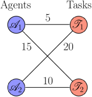
(a) Assignment graph

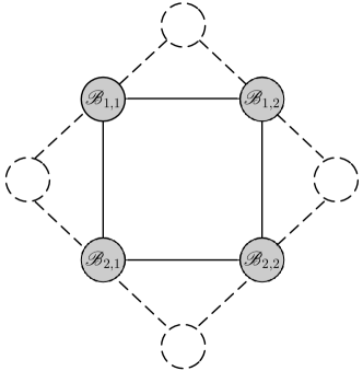
(b) Communication between brokers

Fig. 1: (a) shows the assignment graph with agents $\mathscr{A}_{1}$ and $\mathscr{A}_{2}$ in blue, tasks $\mathscr{T}_{1}$ and $\mathscr{T}_{2}$ in red, and the benefit of a potential assignment as edge weights. (b) shows the connectivity among brokers. Broker $\mathscr{B}_{i,j}$ is responsible for determining the potential assignment of task $\mathscr{T}_{j}$ to agent $\mathscr{A}_{i}$. The dashed nodes represent the virtual brokers whose states correspond to the components of the Lagrange multipliers $z$ in (27), see Remark 5.

We consider an assignment problem with $2$ agents (denoted by $\mathscr{A}_{1}$ and $\mathscr{A}_{2}$) and $2$ tasks (denoted by $\mathscr{T}_{1}$ and $\mathscr{T}_{2}$) as shown in Figure 1(a). The assignment problem is to be solved by a set of $4$ brokers as shown in Figure 1(b). In general, the number of brokers is the number of edges in the assignment graph. Broker $\mathscr{B}_{i,j}$ is responsible for determining the potential assignment of task $\mathscr{T}_{j}$ to agent $\mathscr{A}_{i}$ and has state $x_{i,j}\in\{0,1\}$. Here, $x_{i,j}=1$ means that task $\mathscr{T}_{j}$ is assigned to agent $\mathscr{A}_{i}$ (with associated benefit $c_{i,j}\in\mathbb{R}_{\geq 0}$) and $x_{i,j}=0$ means that they are not assigned to each other. We formulate the multi-agent assignment problem as the following optimization problem,

(29a) $$\max \quad c_{1,1}x_{1,1}+c_{1,2}x_{1,2}+c_{2,1}x_{2,1}+c_{2,2}x_{2,2}$$

(29b) s.t. $$\quad x_{1,1}+x_{1,2}=1$$

(29c) $$\quad x_{2,1}+x_{2,2}=1$$

(29d) $$\quad x_{1,1}+x_{2,1}=1$$

(29e) $$\quad x_{1,2}+x_{2,2}=1$$

(29f) $$\quad x_{1,1},x_{1,2},x_{2,1},x_{2,2}\in\{0,1\}.$$

Constraints (29b)-(29c) (resp. (29d)-(29e)) ensure that each agent (resp. task) is assigned to one and only one task (resp. agent). Note that the connectivity between brokers shown in Figure 1(b) is consistent with the requirements for a distributed implementation as specified by the constraint equations of (29). It is known, see e.g., [23], that the relaxation $x_{i,j}\geq 0$ of the constraints (29f) gives rise to a linear program with an optimal solution that satisfies $x_{i,j}\in\{0,1\}$. Thus, for our purposes, we solve instead the following linear program

(30a) $$\min \quad-5x_{1,1}-15x_{1,2}-20x_{2,1}-10x_{2,2}$$

(30b) s.t. $$\quad x_{1,1}+x_{1,2}=1$$

(30c) $$\quad x_{2,1}+x_{2,2}=1$$

(30d) $$\quad x_{1,1}+x_{2,1}=1$$

(30e) $$\quad x_{1,2}+x_{2,2}=1$$

(30f) $$\quad x_{1,1},x_{1,2},x_{2,1},x_{2,2}\geq 0,$$

where we have also converted the maximization into a minimization by considering the negative of the objective function and substituted the values of the benefits given in Figure 1(a). Clearly, the linear program (30) is in standard form. Its solution set is $\mathcal{X}=\{x^{*}\}$, with $x^{*}=(x_{1,1}^{*},x_{1,2}^{*},x_{2,1}^{*},x_{2,2}^{*})=(0,1,1,0)$, corresponding to the optimal assignment consisting of the pairings $(\mathscr{A}_{1},\mathscr{T}_{2})$ and $(\mathscr{A}_{2},\mathscr{T}_{1})$.

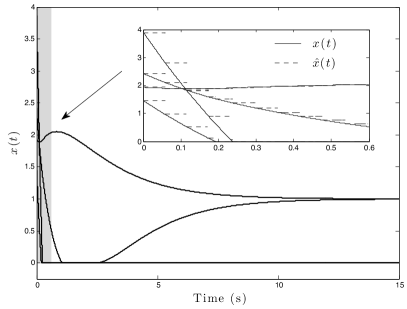
(a) Broker state trajectories

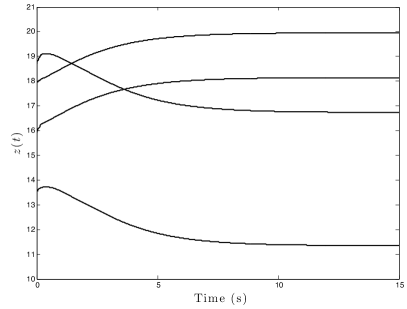
(b) Virtual broker state trajectories

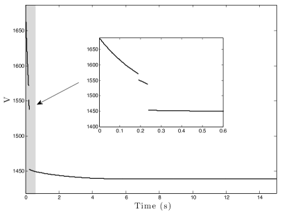
(c) Evolution of $V$

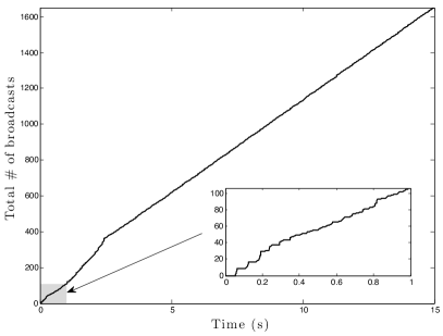
(d) Cumulative number of broadcasts

Fig. 2: Simulation results of brokers implementing (27) to solve the multi-agent assignment problem (30). (a) shows the state trajectories of the brokers, with an inlay displaying the transient response in detail. The brokers’ state is $x=(x_{1,1},x_{1,2},x_{2,1},x_{2,2})$ and the inlay also shows the evolution of the broadcast states, $\hat{x}=(\hat{x}_{1,1},\hat{x}_{1,2},\hat{x}_{2,1},\hat{x}_{2,2})$ in dashed lines. The aggregate of the brokers’ states converge to the unique solution $\mathcal{X}=\{(0,1,1,0)\}$. (b) shows the evolution of the virtual brokers’ states. The Lyapunov function $V$ is discontinuous but decreasing, as evidenced in (c). The cumulative number of broadcasts appears roughly linear and the execution is clearly persistently flowing. Each inlay shows the transient in detail.

Figure 2 shows the group of brokers executing the distributed coordination algorithm (27) with event-triggered communication. Figure 3 illustrates the algorithm performance in the presence of additive white noise on the state broadcasts. The convergence in this case shows the algorithm robustness to sufficiently small disturbances, as pointed out in Remark 14.

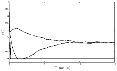
(a) Noisy broker state trajectories

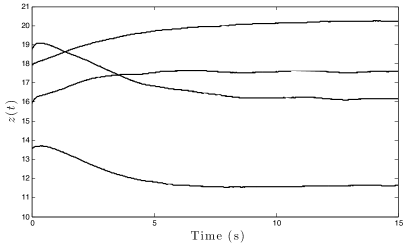
(b) Noisy virtual broker state trajectories

Fig. 3: Simulation results of brokers implementing (27) to solve the multi-agent assignment problem (30) under additive noise in the communication channels. In this simulation, broadcasts of information are corrupted by noise which is normally distributed with zero mean and standard deviation $1$. The network state converges to a neighborhood of the optimal solution and the optimal assignment can easily be deduced.

8 Conclusions and future work

We have studied the design of distributed algorithms for networks of agents that seek to collectively solve linear programs in standard form and rely on discrete-time communication. Our algorithmic solution has agents executing a distributed continuous-time dynamics and deciding in an opportunistic and autonomous way when to broadcast updated state information to their neighbors. Our methodology combines elements from linear programming, switched and hybrid systems, event-triggered control, and Lyapunov stability theory to provide provably correct centralized and distributed strategies. We have rigorously characterized the asymptotic convergence of persistently flowing executions to a solution of the linear program. We have also identified a sufficient condition for executions to be persistently flowing, and based on it, we conjecture that they all are. Future work will be devoted to establish that all solutions are persistently flowing, rigorously characterize the input-to-state stability properties of the proposed algorithm, extend our approach to event-triggered strategies for general switched systems, and implement the results on a multi-agent testbed.

The following two results are used extensively in the proof of Proposition 8 and elsewhere in the paper.

Lemma 15.

(Young’s inequality [10]). Let $d_{1},d_{2}\in\mathbb{N}$ and $\mu\in\mathbb{R}^{d_{1}}$, $M\in\mathbb{R}^{d_{1}\times d_{2}}$, $\nu\in\mathbb{R}^{d_{2}}$. Then, for any $\kappa>0$,

$$\mu^{T}M\nu \leq\frac{\kappa}{2}\nu^{T}M^{T}M\nu+\frac{1}{2\kappa}\mu^{T}\mu.$$

Theorem 16.

(Cauchy Interlacing Theorem [13, Theorem 4.3.15]). For a matrix $0\preceq A\in\mathbb{R}^{d\times d}$, let $0\leq\lambda_{1}\leq\dots\leq\lambda_{d}$ denote its eigenvalues. For $p\in\{1,\dots,d\}$, let $A_{p}$ be the matrix obtained by zeroing out the $p^{\text{th}}$ row and column of $A$, and let $0=\mu_{1}\leq\dots\leq\mu_{d}$ denote its eigenvalues. Then $\mu_{1}\leq\lambda_{1}\leq\mu_{2}\leq\lambda_{2}\leq\dots\leq\mu_{d}\leq\lambda_{d}$.

References

• [1] D. P. Bertsekas and D. A. Castañón, Parallel synchronous and asynchronous implementations of the auction algorithm, Parallel Computing, 17 (1991), pp. 707–732.
• [2] D. P. Bertsekas and J. N. Tsitsiklis, Parallel and Distributed Computation: Numerical Methods, Athena Scientific, 1997.
• [3] S. Boyd and L. Vandenberghe, Convex Optimization, Cambridge University Press, 2009.
• [4] M. Burger, G. Notarstefano, F. Bullo, and F. Allgower, A distributed simplex algorithm for degenerate linear programs and multi-agent assignment, Automatica, 48 (2012), pp. 2298–2304.
• [5] J. Cortés, Distributed algorithms for reaching consensus on general functions, Automatica, 44 (2008), pp. 726–737.
• [6] D. Feijer and F. Paganini, Stability of primal-dual gradient dynamics and applications to network optimization, Automatica, 46 (2010), pp. 1974–1981.
• [7] B. Gharesifard and J. Cortés, Distributed continuous-time convex optimization on weight-balanced digraphs, IEEE Transactions on Automatic Control, 59 (2014), pp. 781–786.
• [8] R. Goebel, R. G. Sanfelice, and A. R. Teel, Hybrid dynamical systems, IEEE Control Systems Magazine, 29 (2009), pp. 28–93.
• [9]  , Hybrid Dynamical Systems: Modeling, Stability, and Robustness, Princeton University Press, 2012.
• [10] G. H. Hardy, J. E. Littlewood, and G. Polya, Inequalities, Cambridge University Press, Cambridge, UK, 1952.
• [11] W. P. M. H. Heemels, K. H. Johansson, and P. Tabuada, An introduction to event-triggered and self-triggered control, in IEEE Conf. on Decision and Control, Maui, HI, 2012, pp. 3270–3285.
• [12] J. P. Hespanha, Uniform stability of switched linear systems: Extensions of LaSalle’s Invariance Principle, IEEE Transactions on Automatic Control, 49 (2004), pp. 470–482.
• [13] R. A. Horn and C. R. Johnson, Matrix Analysis, Cambridge University Press, 1985.
• [14] B. Johansson, T. Keviczky, M. Johansson, and K. H. Johansson, Subgradient methods and consensus algorithms for solving convex optimization problems, in IEEE Conf. on Decision and Control, Cancun, Mexico, 2008, pp. 4185–4190.
• [15] S. S. Kia, J. Cortés, and S. Martínez, Distributed convex optimization via continuous-time coordination algorithms with discrete-time communication, Automatica, (2014). Submitted.
• [16] D. Liberzon, Switching in Systems and Control, Systems & Control: Foundations & Applications, Birkhäuser, 2003.
• [17] O. L. Mangasarian and R. R. Meyer, Nonlinear perturbation of linear programs, SIAM Journal on Control and Optimization, 17 (1979), pp. 745–752.
• [18] M. Mazo Jr. and P. Tabuada, Decentralized event-triggered control over wireless sensor/actuator networks, IEEE Transactions on Automatic Control, 56 (2011), pp. 2456–2461.
• [19] A. Nedic and A. Ozdaglar, Distributed subgradient methods for multi-agent optimization, IEEE Transactions on Automatic Control, 54 (2009), pp. 48–61.
• [20] M. G. Rabbat and R. D. Nowak, Quantized incremental algorithms for distributed optimization, IEEE Journal on Selected Areas in Communications, 23 (2005), pp. 798–808.
• [21] D. Richert and J. Cortés, Robust distributed linear programming, IEEE Transactions on Automatic Control, (2013). Submitted. Available at http://carmenere.ucsd.edu/jorge.
• [22] S. Samar, S. Boyd, and D. Gorinevsky, Distributed estimation via dual decomposition, in European Control Conference, Kos, Greece, July 2007, pp. 1511–1516.
• [23] A. Schrijver, Theory of Linear and Integer Programming, Wiley, New York, 2000.
• [24] P. Wan and M. D. Lemmon, Event-triggered distributed optimization in sensor networks, in Symposium on Information Processing of Sensor Networks, San Francisco, CA, 2009, pp. 49–60.
• [25] X. Wang and M. D. Lemmon, Event-triggering in distributed networked control systems, IEEE Transactions on Automatic Control, 56 (2011), pp. 586–601.
• [26] E. Wei and A. Ozdaglar, Distributed alternating direction method of multipliers, in IEEE Conf. on Decision and Control, Maui, HI, 2012, pp. 5445–5450.
• [27] L. Xiao, M. Johansson, and S. P. Boyd, Simultaneous routing and resource allocation via dual decomposition, IEEE Transactions on Communications, 52 (2004), pp. 1136–1144.
• [28] M. Zhu and S. Martínez, An approximate dual subgradient algorithm for distributed non-convex constrained optimization, IEEE Transactions on Automatic Control, 58 (2013), pp. 1534–1539.