The geometry of kernelized spectral clustering

Abstract

Clustering of data sets is a standard problem in many areas of science and engineering. The method of spectral clustering is based on embedding the data set using a kernel function, and using the top eigenvectors of the normalized Laplacian to recover the connected components. We study the performance of spectral clustering in recovering the latent labels of i.i.d. samples from a finite mixture of nonparametric distributions. The difficulty of this label recovery problem depends on the overlap between mixture components and how easily a mixture component is divided into two nonoverlapping components. When the overlap is small compared to the indivisibility of the mixture components, the principal eigenspace of the population-level normalized Laplacian operator is approximately spanned by the square-root kernelized component densities. In the finite sample setting, and under the same assumption, embedded samples from different components are approximately orthogonal with high probability when the sample size is large. As a corollary we control the fraction of samples mislabeled by spectral clustering under finite mixtures with nonparametric components.

FLA

, and T1Supported by a Graduate Research Fellowship from the NSF—Grant number DGE-1106400. T2Supported by NSF Grants CIF-31712-23800, and DMS-11-07000. T3Supported by NSF Grants DMS-11-07000, DMS-11-60319 (FRG), CDS&E-MSS 1228246, ARO Grant W911NF-11-1-0114 and the Center for Science of Information (CSoI), an US NSF Science and Technology Center, under Grant agreement CCF-0939370.

1 Introduction

In the past decade, spectral methods have emerged as a powerful collection of nonparametric tools for unsupervised learning, or clustering. How can we recover information about the geometry or topology of a distribution from its samples? Clustering algorithms attempt to answer the most basic form of this question. One way in which to understand spectral clustering is as a relaxation of the NP-hard problem of searching for the best graph-cut. Spectral graph partitioning—using the eigenvectors of a matrix to find graph cuts—originated in the early 1970s with the work of Fiedler fiedler and of Donath and Hoffman donathhoffman . Spectral clustering was introduced in machine learning, with applications to clustering data sets and computing image segmentations (e.g., shimalik , ng , shimeila ). The past decade has witnessed an explosion of different spectral clustering algorithms. One point of variation is that some use the eigenvectors of the kernel matrix daspec , kerneleca , donathhoffman , or adjacency matrix in the graph setting, whereas others use the eigenvectors of the normalized Laplacian matrix ng , shimeila , shimalik , fiedler . This division goes all the way back to the work of Donath and Hoffman, who proposed using the adjacency matrix, and of Fiedler, who proposed using the normalized Laplacian matrix.

In its modern and most popular form, the spectral clustering algorithm ng , shimalik involves two steps: first, the eigenvectors of the normalized Laplacian are used to embed the dataset, and second, the $K$-means clustering algorithm is applied to the embedded dataset. The normalized Laplacian embedding is an attractive preprocessing step because the transformed clusters tend to be linearly separable. Ng et al. ng show that, under certain conditions on the empirical kernel matrix, an embedded dataset will cluster tightly around well-separated points on the unit sphere. Their results apply to a fixed dataset, and do not model the underlying distribution of the data. Recently Yan et al. yan derived an expression for the fraction of data misclustered by spectral clustering by computing an analytical expression for the second eigenvector of the Laplacian. They assumed that the similarity matrix is a small perturbation away from the ideal block diagonal case.

The embedding defined by the normalized Laplacian has also been studied in the context of manifold learning, where the primary focus has been convergence of the underlying eigenvectors. This work is motivated in part by the fact that spectral properties of the limiting Laplace–Beltrami operator have long been known to shed light on the connectivity of a manifold cheeger . The Laplacian eigenmaps of Belkin and Niyogi eigenmap reconstruct Laplace–Beltrami eigenfunctions from sampled data. Koltchinskii and Giné kolgine analyze the convergence of the empirical graph Laplacian to the Laplace–Beltrami operator at a fixed point in the manifold. von Luxburg and Belkin luxburg establish consistency for the embedding in as much as the eigenvectors of the Laplacian matrix converge uniformly to the eigenfunctions of the Laplacian operator. Rosasco et al. rosasco provide simpler proofs of this convergence, and in part, our work sharpens these results by removing an unnecessary smoothness assumption on the kernel function.

In this paper, we study spectral clustering in the context of a nonparametric mixture model. The study of spectral clustering under nonparametric mixtures was initiated by Shi et al. daspec . One of their theorems characterizes the top eigenfunction of a kernel integral operator, showing that it does not change sign. One difficulty in using the eigenfunctions of a kernel integral operator to separate mixture components is that several of the top eigenfunctions may correspond to a single mixture component (e.g., one with a larger mixture weight). They propose that eigenfunctions of the kernel integral operator that approximately do not change sign correspond to different mixture components. However, their analysis does not deal with finite datasets nor does it provide bounds on the fraction of points misclustered.

The main contribution of this paper is an analysis of the normalized Laplacian embedding of i.i.d. samples from a finite mixture with nonparametric components. We begin by providing a novel and useful characterization of the principal eigenspace of the population-level normalized Laplacian operator: more precisely, when the mixture components are indivisible and have small overlap, the eigenspace is close to the span of the square root kernelized component densities. We then use this characterization to analyze the geometric structure of the embedding of a finite set of i.i.d. samples. Our main result is to establish a certain geometric property of nonparametric mixtures referred to as orthogonal cone structure. In particular, we show that when the mixture components are indivisible and have small overlap, embedded samples from different components are almost orthogonal with high probability. We then prove that this geometric structure allows $K$-means to correctly label most of the samples. Our proofs rely on techniques from operator perturbation theory, empirical process theory and spectral graph theory.

The remainder of this paper is organized as follows. In Section 2, we set up the problem of separating the components of a mixture distribution. We state our main results and explore some of their consequences in Section 3. We prove our main results in Section 4, deferring the proofs of several supporting lemmas to the supplementary material SchiebingerWainwrightYu14Sup .

Notation

For a generic distribution $\mathbb{P}$ on a measurable space ${\mathcal{X}}$, we denote the Hilbert space of real-valued square integrable functions on ${\mathcal{X}}$ by ${L^{2}(\mathbb{P})}$. The ${L^{2}(\mathbb{P})}$ inner product is given by ${\langle f,g\rangle}_{\mathbb{P}}=\int f(x)g(x)\,d\mathbb{P}(x)$, and it induces the norm $\|f\|_{\mathbb{P}}$. The norm ${\|f\|_{\infty}}$ is the supremum of the function $f$, up to sets of measure zero, where the relevant measure is understood from context. The Hilbert–Schmidt norm of an operator $\mathbf{T}\dvtx{L^{2}(\mathbb{P})}\to{L^{2}(\mathbb{P})}$ is $|\!|\!|\mathbf{T}|\!|\!|_{\mathrm{HS}}$, and the operator norm is $|\!|\!|\mathbf{T}|\!|\!|_{\mathrm{op}}$. The complement of a set $B$ is denoted by $B^{c}$. See Appendix D (supplementary material SchiebingerWainwrightYu14Sup ) for an additional list of symbols.

2 Background and problem set-up

We begin by introducing the family of nonparametric mixture models analyzed in this paper, and then provide some background on kernel functions, spectral clustering and Laplacian operators.

2.1 Nonparametric mixture distributions

For some integer $K\geq 2$, let $\{\mathbb{P}_{m}\}_{m=1}^{K}$ be a collection of probability measures on a compact space ${\mathcal{X}}$, and let the weights $\{w_{m}\}_{m=1}^{K}$ belong to the relative interior of the probability simplex in ${\mathbb{R}}^{K}$—that is, $w_{m}\in(0,1)$ for all $m=1,\ldots,K$, and $\sum_{m=1}^{K}w_{m}=1$. This pair specifies a finite nonparametric mixture distribution via the convex combination

$$\bar{\mathbb{P}} := \sum_{m=1}^{K}w_{m}\mathbb{P}_{m}.$$ (1)

We refer to ${\{\mathbb{P}_{m}\}_{m=1}^{K}}$ and ${\{w_{m}\}_{m=1}^{K}}$ as the mixture components and mixture weights, respectively. The family of models (1) is nonparametric, because the mixture components are not constrained to any particular parametric family.

A random variable ${\bar{X}}\sim\bar{\mathbb{P}}$ can be obtained by first drawing a multinomial random variable ${Z}\sim\operatorname{Multinomial}(w_{1},\ldots,w_{K})$, and conditioning on the event $\{{Z}=m\}$, drawing a variable from mixture component $\mathbb{P}_{m}$. Consequently, given a collection of samples $\{X_{i}\}_{i=1}^{n}$ drawn i.i.d. from $\bar{\mathbb{P}}$, there is an underlying set of latent labels $\{{Z}_{i}\}_{i=1}^{n}$. Thus in the context of a mixture distribution, the clustering problem can be formalized as recovering these latent labels based on observing only the unlabeled samples $\{X_{i}\}_{i=1}^{n}$.

Of course, this clustering problem is ill defined whenever $\mathbb{P}_{j}=\mathbb{P}_{k}$ for some $j\neq k$. More generally, recovery of labels becomes more difficult as the overlap of any pair $\mathbb{P}_{j}$ and $\mathbb{P}_{k}$ increases, or if it is “easy” to divide any component into two nonoverlapping distributions. This intuition is formalized in our definition of the overlap and indivisibility parameters in Section 3.1 to follow.

2.2 Kernels and spectral clustering

We now provide some background on spectral clustering methods and the normalized Laplacian embedding. A kernel $k$ associated with the space ${\mathcal{X}}$ is a symmetric, continuous function $k\dvtx{\mathcal{X}}\times{\mathcal{X}}\to(0,\infty)$. A kernel is said to be positive semidefinite if for any integer ${n}\geq 1$ and elements $x_{1},\ldots,x_{n}\in{\mathcal{X}}$, the kernel matrix $A\in\mathbb{R}^{{n}\times{n}}$ with entries $A_{ij}=k(x_{i},x_{j})/n$ is positive semidefinite. Throughout we consider a fixed but arbitrary positive semidefinite kernel function. In application to spectral clustering, one purpose of a kernel function is to provide a measure of the similarity between data points. A canonical example is the Gaussian kernel $k(x,x^{\prime})=\exp(-\|x-x^{\prime}\|_{2}^{2})$; it is close to $1$ for vectors $x$ and $x^{\prime}$ that are relatively close, and decays to zero for pairs that are far apart.

Let us now describe the normalized Laplacian embedding, which is a standard part of many spectral clustering routines. Given ${n}$ i.i.d. samples $\{X_{i}\}_{i=1}^{n}$ from $\bar{\mathbb{P}}$, the associated kernel matrix $A\in{\mathbb{R}}^{{n}\times{n}}$ has entries $A_{ij}=\frac{1}{{n}}k(X_{i},X_{j})$. The normalized Laplacian matrix is obtained by rescaling the kernel matrix by its row sums, namely

$$L=D^{-1/2}AD^{-1/2},$$ (2)

where $D$ is a diagonal matrix with entries $D_{ii}=\sum_{j=1}^{n}A_{ij}$. Since $L$ is a symmetric matrix by construction, it has an orthonormal basis of eigenvectors, and we let $\{v_{1},\ldots,v_{K}\}$ denote the eigenvectors corresponding to the largest $K$ eigenvalues of $L$. The normalized Laplacian embedding is defined on the basis of these eigenvectors: it is the map $\Phi_{\mathcal{V}}\dvtx\{X_{1},\ldots,X_{n}\}\to\mathbb{R}^{K}$ defined by

$$\Phi_{\mathcal{V}}(X_{i}) := (v_{1i},\ldots,v_{Ki}).$$ (3)

A typical form of spectral clustering consists of the following two steps. First, compute the normalized Laplacian, and map each data point $X_{i}$ to a $K$-vector via the embedding (3). The second step is to apply a standard clustering method (such as $K$-means clustering) to the embedded data points. The conventional rationale for the second step is that the embedding step typically helps reveal cluster structure in the data set, so that it can be found by a relatively simple algorithm. The goal of this paper is to formalize the sense in which the normalized Laplacian embedding (3) has this desirable property.

We do so by first analyzing the population operator that underlies the normalized Laplacian matrix. It is defined by the normalized kernel function

$${\bar{k}}(x,y) := \frac{1}{\bar{q}(x)}k(x,y)\frac{1}{\bar{q}(y)},$$ (4)

where $\bar{q}(y)=\sqrt{\int k(x,y)\,d\bar{\mathbb{P}}(x)}$. Note that this kernel function can be seen as a continuous analog of the normalized Laplacian matrix (2).

The normalized kernel function in conjunction with the mixture defines the normalized Laplacian operator $\bar{\mathbf{T}}\dvtx L^{2}(\bar{\mathbb{P}})\rightarrow L^{2}(\bar{\mathbb{P}})$ given by

$$(\bar{\mathbf{T}}f)(\cdot) := \int{\bar{k}}(\cdot,y)f(y)\,d\bar{\mathbb{P}}(y).$$ (5)

Under suitable regularity conditions (see Appendix C.1 (supplementarymaterial SchiebingerWainwrightYu14Sup ) for details), this operator has an orthonormal set ofeigenfunctions—with eigenvalues in $[0,1]$—and our main results relate these eigenfunctions to the underlying mixture components $\{{\mathbb{P}}_{m}\}_{m=1}^{K}$.

3 Analysis of the normalized Laplacian embedding

This section is devoted to the statement of our main results, and discussion of their consequences. These results involve a few parameters of the mixture distribution, including its overlap and indivisibility parameters, which are defind in Section 3.1. Our first main result (Theorem 1 in Section 3.2) characterizes the principal eigenspace of the population-level normalized Laplacian operator (5), showing that it approximately spanned by the square root kernelized densities of the mixture components, as defined in Section 3.1. Our second main result (Theorem 2 in Section 3.3) provides a quantitative description of the angular structure in the normalized Laplacian embedding of a finite sample from a mixture distribution.

3.1 Cluster similarity, coupling and indivisibility parameters

In this section, we define some parameters associated with any nonparametric mixture distribution, as viewed through the lens of a given kernel. These quantities play an important role in our main results, as they reflect the intrinsic difficulty of the clustering problem.

Our first parameter is the similarity index of the mixture components $\{{\mathbb{P}}_{m}\}_{m=1}^{K}$. For any pair of distinct indices $\ell\neq m$, the ratio

$${\mathcal{S}}({\mathbb{P}}_{\ell},{\mathbb{P}}_{m}) := \frac{\int_{{\mathcal{X}}}\int_{{\mathcal{X}}}k(x,y)\,d{\mathbb{P}}_{m}(x)\,d{\mathbb{P}}_{\ell}(y)}{\int_{{\mathcal{X}}}\int_{{\mathcal{X}}}k(x,y)\,d{{\bar{\mathbb{P}}}}(x)\,d{\mathbb{P}}_{\ell}(y)}$$

is a kernel-dependent measure of the expected similarity between the clusters indexed by ${\mathbb{P}}_{\ell}$ and ${\mathbb{P}}_{m}$, respectively. Note that ${\mathcal{S}}$ is not symmetric in its arguments. The maximum similarity over all mixture components

$$\mathcal{S}_{\max}({\bar{\mathbb{P}}}) := \mathop{\max_{\ell,m=1,\ldots,K}}_{\ell\neq m}{\mathcal{S}}({\mathbb{P}}_{\ell},{\mathbb{P}}_{m})$$ (6)

measures the overlap between mixture components with respect to the kernel $k$.

Our second parameter, known as the coupling parameter, is defined in terms of the square root kernelized densities of the mixture components. More precisely, given any distribution $\mathbb{P}$, its square root kernelized density is the function $q\in{L^{2}(\mathbb{P})}$ given by

$$q(x) := \sqrt{\int k(x,y)\,d\mathbb{P}(y)}.$$ (7)

In particular, we denote the square root kernelized density of the mixture distribution $\bar{\mathbb{P}}$ by $\bar{q}$, and those of the mixture components $\{\mathbb{P}_{m}\}_{m=1}^{K}$ by $\{q_{m}\}_{m=1}^{K}$. In analogy with the normalized kernel function ${\bar{k}}$ from equation (4), we also define a normalized kernel for each mixture component, namely

$$k_{m}(x,y) := \frac{k(x,y)}{q_{m}(x)q_{m}(y)}\qquad\mbox{for $m=1,\ldots,K$.}$$ (8)

The coupling parameter

$${{\mathcal{C}}({\bar{\mathbb{P}}})} := \max_{m=1,\ldots,K}{\|{k_{m}-w_{m}{\bar{k}}}\|^{2}_{\mathbb{P}_{m}\otimes\mathbb{P}_{m}}}$$ (9)

measures the coupling of the spaces ${L^{2}(\mathbb{P}_{m})}$ with respect to $\bar{\mathbf{T}}$. In particular, when ${{\mathcal{C}}({\bar{\mathbb{P}}})}=0$, then the normalized Laplacian can be decomposed as the sum

$$\bar{\mathbf{T}} = \sum_{m=1}^{K}w_{m}\mathbf{T}_{m},$$ (10)

where $(\mathbf{T}_{m}f)(y)=\int f(x)k_{m}(x,y)\,d\mathbb{P}_{m}(x)$ is the operator defined by the normalized kernel $k_{m}$. When the coupling parameter is no longer exactly zero but still small, then decomposition (10) still holds in an approximate sense.

Our final parameter measures how easy or difficult it is to “split” any given mixture component $\mathbb{P}_{m}$ into two or more parts. If this splitting can be done easily for any component, then the mixture distribution will be hard to identify, since there is an ambiguity as to whether $\mathbb{P}_{m}$ defines one component or multiple components. In order to formalize this intuition, for a distribution $\mathbb{P}$ and for a measurable subset $S\subset{\mathcal{X}}$, we introduce the shorthand notation $p(S)=\int_{S}\int_{\mathcal{X}}k(x,y)\,d\mathbb{P}(x)\,d\mathbb{P}(y)$. With this notation, the indivisibility of $\mathbb{P}$ is

$${\Gamma({\mathbb{P}})} := \inf_{S}\frac{p({\mathcal{X}})\int_{S}\int_{S^{c}}k(x,y)\,d\mathbb{P}(x)\,d\mathbb{P}(y)}{p(S)p(S^{c})},$$ (11)

where the infimum is taken over all measurable subsets $S$ such that $p(S)\in(0,1)$. The indivisibility parameter $\Gamma_{\min}({\bar{\mathbb{P}}})$ of a mixture distribution ${\bar{\mathbb{P}}}$ is the minimum indivisibility of its mixture components

$$\Gamma_{\min}({\bar{\mathbb{P}}}) := \min_{m=1,\ldots,K}{\Gamma({\mathbb{P}_{m}})}.$$ (12)

Our results in the next section apply when the similarity ${\mathcal{S}}_{\max}({\bar{\mathbb{P}}})$ and coupling ${{\mathcal{C}}({\bar{\mathbb{P}}})}$ are small compared to the indivisibility $\Gamma_{\min}({\bar{\mathbb{P}}})$. Some examples help illustrate when this is the case.

Example 1.

Consider the one-dimensional triangular density function

$$g_{{\mathbb{T}}_{\mu}}(x):=\cases{x-\mu+1,&\quad if $x\in(\mu-1,\mu)$;\cr-x+\mu+1,&\quad if $x\in(\mu,\mu+1)$;\cr 0,&\quad otherwise,}$$

with location $\mu>0$. We denote corresponding distribution by ${\mathbb{T}}_{\mu}$. In this example we calculate the similarity, coupling and indivisibility parameters for the mixture of triangular distributions $\bar{\mathbb{T}}:=\frac{1}{2}{\mathbb{T}}_{0}+\frac{1}{2}{\mathbb{T}}_{\mu}$ and the uniform kernel $k_{\nu}(x,y)=\frac{1}{2\nu}\mathbf{1}\{|x-y|\leq\nu\}$ with bandwidth $\nu\in(0,1)$.

Similarity

It is straightforward to calculate the similarity parameter ${\mathcal{S}}_{\max}(\bar{\mathbb{T}})$ by solving a few simple integrals. We find that

$$\mathcal{S}_{\max}(\bar{\mathbb{T}})=\frac{2(2+\nu-\mu)_{+}^{4}}{\nu(16-8\nu^{2}+3\nu^{3})+(2+\nu-\mu)_{+}^{4}}.$$

Coupling

To compute the coupling parameter, we must compute the kernelized densities of ${\mathbb{T}}_{0}$ and ${\mathbb{T}}_{\mu}$, and the normalized kernel functions $k_{1}(x,y)$ and ${\bar{k}}(x,y)$. Some calculation yields the following equation for the kernelized density:

$$q_{1}^{2}(x)=\cases{\displaystyle\frac{(1+\nu-x)^{2}}{4\nu},&\quad if $x\in(-1-\nu,-1+\nu)$,\vspace*{5pt}\cr\displaystyle 1-\frac{\nu}{2}-\frac{x^{2}}{2\nu},&\quad if $x\in(-\nu,\nu)$,\vspace*{5pt}\cr\displaystyle\frac{(1+\nu+x)^{2}}{4\nu},&\quad if $x\in(1-\nu,1+\nu)$,\vspace*{5pt}\cr\displaystyle g_{{\mathbb{T}}_{0}}(x),&\quad otherwise.}$$ (13)

As can be seen in Figure 1, the kernelized density $q_{1}^{2}(x)$ of ${\mathbb{T}}_{0}$ is a smoothed version of $g_{{\mathbb{T}}_{0}}(x)$ that interpolates quadratically around the nondifferentiable points of $g_{{\mathbb{T}}_{0}}(x)$.

Figure 1: The kernelized density $q_{1}^{2}(x)$ of equation (13) with $\nu=0.05$.

The kernelized density of ${\mathbb{T}}_{\mu}$ has the same shape as that of ${\mathbb{T}}_{0}$ but is shifted by $\mu$. In particular,

$$q_{2}^{2}(x)=q_{1}^{2}(x-\mu).$$

Therefore the normalized kernels satisfy $k_{1}(x,y)=\frac{1}{2}{\bar{k}}(x,y)$ for $x,y\in(-1,\mu-1-\nu)$. By upper bounding the integrand over the remaining region, we find that

$${{\mathcal{C}}(\bar{\mathbb{T}})}^{2}=\int\!\!\!\int(k_{1}-{{\bar{k}}}/{2})^{2}\,d\mathbb{P}_{1}(x,y)\leq{2(2+\nu-\mu)_{+}}.$$

Indivisibility

It is straightforward to calculate the indivisibility $\Gamma({\mathbb{T}}_{\mu})$. For any $\nu\in(0,1)$ and $\mu\in\mathbb{R}$, the set $S$ defining ${\Gamma({{\mathbb{T}}_{\mu}})}$ is $S=(\mu,\infty)$. Hence by solving a few simple integrals, we find that

$${\Gamma({{\mathbb{T}}_{\mu}})}=\frac{2(6-\nu)(2-\nu)\nu}{16-8\nu^{2}+3\nu^{3}}.$$

Note that ${\Gamma({{\mathbb{T}}_{\mu}})}$ does not depend on $\mu$. Therefore the indivisibility of $\bar{\mathbb{T}}:=\frac{1}{2}{\mathbb{T}}_{0}+\frac{1}{2}{\mathbb{T}}_{\mu}$ is

$$\Gamma_{\min}(\bar{\mathbb{T}})={\Gamma({{\mathbb{T}}_{\mu}})}={\Gamma({{\mathbb{T}}_{0}})}.$$

It is instructive to consider the indivisibility of the following poorly defined two-component mixture:

$$\bar{\mathbb{T}}_{\mathrm{bad}}:=\tfrac{1}{2}\mathbb{P}_{\mathrm{bad}}(\mu)+\tfrac{1}{2}{\mathbb{T}}_{2\mu},$$

where $\mathbb{P}_{\mathrm{bad}}(\mu)$ is the bimodal component $\mathbb{P}_{\mathrm{bad}}(\mu):=\frac{1}{2}{\mathbb{T}}_{0}+\frac{1}{2}{\mathbb{T}}_{\mu}$. It is easy to verify that for any $\nu\in(0,1)$ and $\mu>2+\nu$, the indivisibility of the bimodal component is $\Gamma(\mathbb{P}_{\mathrm{bad}}(\mu))=0$, and therefore $\Gamma_{\min}(\bar{\mathbb{T}}_{\mathrm{bad}})=0$.

From Example 1 we learn that the similarity ${\mathcal{S}}_{\max}(\bar{\mathbb{T}})$ and coupling ${{\mathcal{C}}(\bar{\mathbb{T}})}$ parameters decrease as the offset $\mu$ increases. Together, these two parameters measure the overlap which our intuition tells us should decrease as $\mu$ increases. On the other hand, the indivisibility parameter $\Gamma_{\min}(\bar{\mathbb{T}})$ is independent of $\mu$.

Our next example is more realistic in the sense that the kernel and mixture components do not have bounded support, and the kernel function is positive semidefinite.

Example 2.

In this example we calculate the similarity, coupling and indivisibility parameters for the mixture of Gaussians $\bar{\mathbb{N}}=\frac{1}{2}\mathbb{N}(0,1)+\frac{1}{2}\mathbb{N}(\mu,1)$ equipped with the Gaussian kernel $k_{\nu}(x,y)=\frac{1}{\sqrt{2\pi}\nu}\exp[-\frac{|x-y|^{2}}{2\nu^{2}}]$.

Similarity

As in the previous example, it is straightforward to calculate the maximal intercluster similarity $\mathcal{S}_{\max}(\bar{\mathbb{N}})$ by solving a handful of Gaussian integrals. We find that

$$\mathcal{S}_{\max}(\bar{\mathbb{N}})=\frac{2\exp({{-\mu^{2}}/(2\nu^{2}+4)})}{1+\exp({{-\mu^{2}}/(2\nu^{2}+4)})}\leq 4e^{{-\mu^{2}}/(2\nu^{2}+4)}.$$ (14)

Coupling

The kernelized density of $\mathbb{N}(0,1)$ is

$$q_{1}^{2}(x)=\frac{1}{\sqrt{\nu^{2}+1}}\exp\biggl{[}{\frac{-x^{2}}{2(\nu^{2}+1)}}\biggr{]},$$

and the kernelized density of $\mathbb{N}(\mu,1)$ is simply the translation $q_{2}^{2}(x)=q_{1}^{2}(x-\mu)$. We can bound the coupling parameter ${{\mathcal{C}}(\bar{\mathbb{N}})}$ by upper bounding the integrand $k_{1}-{\bar{k}}$ over a high-probability compact set (a modification of the trick from Example 1). We show the resulting bound in Figure 2. This (albeit loose) bound captures the exponential decay of ${{\mathcal{C}}(\bar{\mathbb{N}})}$ with $\mu$.

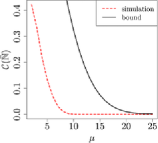
Figure 2: The coupling parameter ${{\mathcal{C}}(\bar{\mathbb{N}})}$ for the mixture of Gaussians with Gaussian kernel and $\nu=2$. The red line displays the simulated value of ${{\mathcal{C}}(\bar{\mathbb{N}})}$ as a function of the offset $\mu$ between mixture components. The black line displays our analytical bound.

Indivisibility

It is straightforward to compute the indivisibility of the unit-variance normal distribution $\mathbb{N}(\mu,1)$ with location $\mu\in\mathbb{R}$. The set defining the indivisibility is $S=(\mu,\infty)$. Solving a handful of Gaussian integrals yields

$$\Gamma_{\min}\bigl{(}\mathbb{N}(\mu,1)\bigr{)}=\frac{2}{\pi}\arctan\bigl{(}{\nu\sqrt{2+\nu^{2}}}\bigr{)}.$$ (15)

We conclude with a counter example, showing that the similarity parameter is not relatively small for the linear kernel $k(x,y)=x\cdot y$.

Example 3.

Consider the mixture ${\bar{\mathbb{P}}}=\frac{1}{2}\mathbb{P}_{1}+\frac{1}{2}\mathbb{P}_{2}$ with components $\mathbb{P}_{1}$ uniform over $(1,2)$ and $\mathbb{P}_{2}$ uniform over $(2+\delta,3+\delta)$. With the linear kernel $k(x,y)=x\cdot y$, we have

$$\mathcal{S}_{\max}({\bar{\mathbb{P}}})=\frac{\int\!\!\!\int xy\,d\mathbb{P}_{1}(x)\,d\mathbb{P}_{2}(y)}{\int\!\!\!\int xy\,d\mathbb{P}_{1}(x)\,d{\bar{\mathbb{P}}}(y)}=\frac{\int y\,d\mathbb{P}_{2}(y)}{\int y\,d{\bar{\mathbb{P}}}(y)}\geq\frac{1}{2}.$$

Since $\Gamma_{\min}({\bar{\mathbb{P}}})$ is always between $0$ and $1$, this calculation demonstrates that the similarity parameter $\mathcal{S}_{\max}({\bar{\mathbb{P}}})$ is never small compared to $\Gamma_{\min}({\bar{\mathbb{P}}})$.

3.2 Population-level analysis

In this section, we present our population-level analysis of the normalized Laplacian embedding. Consider the following two subspaces of ${L^{2}(\bar{\mathbb{P}})}$:

• the subspace $\mathcal{R}\subset{L^{2}(\bar{\mathbb{P}})}$ spanned by the top $K$ eigenfunctions of the normalized Laplacian operator $\bar{\mathbf{T}}$ from equation (5) and

• the span ${\mathcal{Q}}=\operatorname{span}\{q_{1},\ldots,q_{K}\}\subset{L^{2}(\bar{\mathbb{P}})}$ of the square root kernelized densities; see equation (7).

The subspace ${\mathcal{Q}}$ can be used to define a map $\Phi_{{\mathcal{Q}}}\dvtx{\mathcal{X}}\to\mathbb{R}^{K}$ known as the square-root kernelized density embedding, given by

$$\Phi_{{\mathcal{Q}}}(x) := \bigl{(}q_{1}(x),\ldots,q_{K}(x)\bigr{)}.$$ (16)

This map is relevant to clustering, since the vector $\Phi_{{\mathcal{Q}}}(x)$ encodes sufficient information to perform a likelihood ratio test (based on the kernelized densities) for labeling data points.

On the other hand, the subspace $\mathcal{R}$ is important because it is thepopulation-level quantity that underlies spectral clustering. As described in Section 2.2, the first step of spectral clustering involves embedding the data using the eigenvectors of the Laplacian matrix. This procedure can be understood as a way of estimating the population-level Laplacian embedding: more precisely, the map $\Phi_{\mathcal{R}}\dvtx{\mathcal{X}}\to\mathbb{R}^{K}$ given by

$$\Phi_{\mathcal{R}}(x) := \bigl{(}r_{1}(x),\ldots,r_{K}(x)\bigr{)},$$ (17)

where $\{r_{m}\}_{m=1}^{K}$ are the top $K$ eigenfunctions of the kernel operator $\bar{\mathbf{T}}$.

To build intuition, imagine for the moment varying the kernel function so that the kernelized densities converge to the true densities. For example, imagine sending the bandwidth of a Gaussian kernel to $0$. While the kernelized densities approach the true densities, the subspace $\mathcal{R}$ is only a well defined mathematical object for kernels with nonzero bandwidth. Indeed, as the bandwidth shrinks to zero, the eigengap separating the principal eigenspace $\mathcal{R}$ of $\bar{\mathbf{T}}$ from its lower eigenspaces vanishes. For this reason, we analyze an arbitrary but fixed kernel function, and we discuss kernel selection in Section 5.

The goal of this section is to quantify the difference between the two mappings $\Phi_{{\mathcal{Q}}}$ and $\Phi_{\mathcal{R}}$, or equivalently between the underlying subspaces ${\mathcal{Q}}$ and $\mathcal{R}$. We assume that the square root kernelized densities $q_{1},\ldots,q_{K}$ are linearly independent so that ${\mathcal{Q}}$ has the same dimension, $K$, as $\mathcal{R}$. This condition is very mild when the overlap parameters $\mathcal{S}_{\max}(\bar{\mathbb{P}})$ and ${{\mathcal{C}}(\bar{\mathbb{P}})}$ are small. We measure the distance between these subspaces by the Hilbert–Schmidt norm applied to the difference between their orthogonal projection operators,

$$\rho({\mathcal{Q}},\mathcal{R}) := |\!|\!|{\Pi_{{\mathcal{Q}}}}-{\Pi_{\mathcal{R}}}|\!|\!|_{\mathrm{HS}}.$$ (18)

Recall the similarity parameter $\mathcal{S}_{\max}({{\bar{\mathbb{P}}}})$, coupling parameter ${{\mathcal{C}}({\bar{\mathbb{P}}})}$ and indivisibility parameter $\Gamma_{\min}({\bar{\mathbb{P}}})$, as previously defined in equations (6), (9) and (12), respectively. Our main results involve a function of these three parameters and the minimum $w_{\min}:=\min_{m=1,\ldots,K}w_{m}$ of the mixture weights, given by

$$\varphi({\bar{\mathbb{P}}};k) := \frac{\sqrt{K}[\mathcal{S}_{\max}({\bar{\mathbb{P}}})+{{\mathcal{C}}({\bar{\mathbb{P}}})}]^{1/2}}{w_{\min}\Gamma^{2}_{\min}({\bar{\mathbb{P}}})}.$$ (19)

Our first main theorem guarantees that as long as the mixture is relatively well separated, as measured by the difficulty function $\varphi$, then the $\rho$-distance (18) between $\mathcal{R}$ and ${\mathcal{Q}}$ is proportional to $\varphi({\bar{\mathbb{P}}};k)$. Our theorem also involves the quantity

$$b_{\max}:=\max\limits_{m=1,\ldots,K}{\biggl{\|}\int k_{m}(x,y)\,d\mathbb{P}_{m}(y)\biggr{\|}_{\infty}^{2}}.$$

Note that this is simply a constant whenever the kernels $k_{m}$ are bounded.

Theorem 1 ((Population control of subspaces))

For any finite mixture ${\bar{\mathbb{P}}}$ with difficulty function bounded as $\varphi({\bar{\mathbb{P}}};k)\leq[576\sqrt{12+b_{\max}}]^{-1}\Gamma^{2}_{\min}({\bar{\mathbb{P}}})$, the distance between subspaces ${\mathcal{Q}}$ and $\mathcal{R}$ is bounded as

$$\rho({\mathcal{Q}},\mathcal{R}) \leq 16\sqrt{12+{b_{\max}}}\varphi({\bar{\mathbb{P}}};k).$$ (20)

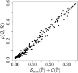
Figure 3: The $\rho$-distance between ${\mathcal{Q}}$ and $\mathcal{R}$ scales linearly with $\mathcal{S}_{\max}({\bar{\mathbb{P}}})+{{\mathcal{C}}({\bar{\mathbb{P}}})}$. Each point corresponds to a different offset $\mu$ between the two Gaussian mixture components from Example 3.

Relationship (20) is easy to understand in the context of translated copies of identical mixture components. Consider the mixture of Gaussians with Gaussian kernel setup in Example 3. Recall from equation (15) that the indivisibility parameter is independent of the offset $\mu$. Hence in this setting relationship (20) simplifies to

$$\rho({\mathcal{Q}},\mathcal{R})\leq c\bigl{[}\mathcal{S}_{\max}({{\bar{\mathbb{P}}}})+{{\mathcal{C}}({\bar{\mathbb{P}}})}\bigr{]}^{1/2}.$$

Figure 3 shows a clear linear relationship between $\rho({\mathcal{Q}},\mathcal{R})$ and ${\mathcal{S}}_{\max}({\bar{\mathbb{P}}})+{{\mathcal{C}}({\bar{\mathbb{P}}})}$, suggesting that it might be possible to remove the square root in the clustering difficulty (19).

One important consequence of relationship (20) stems from geometric structure in the square root kernelized density embedding. When there is little overlap between mixture components with respect to the kernel, the square root kernelized densities are not simultaneously large; that is, $\Phi_{{\mathcal{Q}}}(X)$ will have at most one component much different from zero. Therefore the data will concentrate in tight spikes about the axes. This is illustrated in Figure 4.

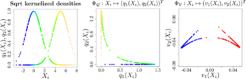
Figure 4: Geometric structure in the square root kernelized density embedding. (Left) square root kernelized densities for a mixture of Gaussians with Gaussian kernel. The color of the $i$th dot indicates the likelihood ratio of the mixture components at $X_{i}$. (Center) data embedded under the square root kernelized density embedding $\Phi_{{\mathcal{Q}}}$, colored by likelihood ratio. (Right) normalized Laplacian embedding of the samples, colored by latent label.

3.3 Finite sample analysis

Thus far, our analysis has been limited to the population level, corresponding to the ideal case of infinitely many samples. We now turn to the case of finite samples. Here an additional level of analysis is required, in order to relate empirical versions (based on the finite collection of samples) to their population analogues. Doing so allows us to show that under suitable conditions, the Laplacian embedding applied to i.i.d. samples drawn from a finite mixture satisfies a certain geometric property, which we call orthogonal cone structure, or OCS for short.

We begin by providing a precise definition of when an embedding $\Phi\dvtx{\mathcal{X}}\rightarrow{\mathbb{R}}^{K}$ reveals orthogonal cone structure. Given a collection of labeled samples $\{X_{i},Z_{i}\}_{i=1}^{n}\subset{\mathcal{X}}\times[K]$ drawn from a $K$-component mixture distribution, we let ${\mathcal{Z}}_{m}=\{i\in[{n}]|Z_{i}=m\}$ denote the subset of samples drawn from mixture component $m=1,\ldots,K$. For any set ${\mathcal{Z}}\subseteq[{n}]=\{1,2,\ldots,{n}\}$, we use $|{\mathcal{Z}}|$ to denote its cardinality. For vectors $u,v\in{\mathbb{R}}^{n}$, we use $\operatorname{angle}(u,v)=\mbox{arccos}\frac{{\langle u,v\rangle}}{\|u\|_{2}\|v\|_{2}}$ to denote the angle between them. With this notation, we have the following:

Definition 1 ([Orthogonal cone structure (OCS)]).

Given parameters $\alpha\in(0,1)$ and $\theta\in(0,\frac{\pi}{4})$, the embedded data set $\{\Phi(X_{i}),Z_{i}\}_{i=1}^{n}$ has $(\alpha,\theta)$-OCS if there is an orthogonal basis $\{e_{1},\ldots,e_{K}\}$ of ${\mathbb{R}}^{K}$ such that

$$\bigl{|}\bigl{\{}i\in[{n}]|\operatorname{angle}\bigl{(}\Phi(X_{i}),e_{m}\bigr{)}<\theta\bigr{\}}\cap{\mathcal{Z}}_{m}\bigr{|} \geq (1-\alpha)|{\mathcal{Z}}_{m}|\qquad\mbox{for all $m=1,\ldots,K$.}$$

In words, a labeled dataset has orthogonal cone structure if most pairs of embedded data points with distinct labels are almost orthogonal. See Figure 5 for an illustration of this property.

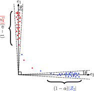
Figure 5: Visualizing $(\alpha,\theta)$-OCS: the labeled set of points plotted above has $(\alpha,\theta)$ orthogonal cone structure with respect to its labeling. The color of each dot indicates the value of the corresponding label ${Z}_{i}\in\{1,2\}$, where $1$ corresponds to red and $2$ to blue. This set of points has $(\alpha,\theta)$-orthogonal cone structure because a fraction $1-\alpha$ of the red points (for which ${Z}_{i}=1$) lie with an angle $\theta$ of $e_{1}$, a fraction $1-\alpha$ blue points (for which ${Z}_{i}=2$) lie with an angle $\theta$ of $e_{2}$ and $e_{1}$ is orthogonal to $e_{2}$.

Our main theorem in the finite sample setting establishes that under suitable conditions, the normalized Laplacian embedding has orthogonal cone structure. In order to state this result precisely, we require a few additional conditions.

Kernel parameters

As a consequence of the compactness of ${\mathcal{X}}$, the kernel function is $b$-bounded, meaning that $k(x,x^{\prime})\in(0,b)$ for all $x,x^{\prime}\in{\mathcal{X}}$. As another consequence, the kernelized densities are lower bounded as $q_{m}(X^{m})\geq r>0$ with ${\bar{\mathbb{P}}}$-probability one. In the following statements, we use $c,{c}_{0},{c}_{1},\ldots$ to denote quantities that may depend on $b$, and $r$ but are otherwise independent of the mixture distribution.

Tail decay

The tail decay of the mixture components enters our finite sample result through the function $\psi\dvtx(0,\infty)\to[0,1]$, defined by

$$\psi(t) := \sum_{m=1}^{K}{\mathbb{P}}_{m}\biggl{[}\frac{q_{m}^{2}(X)}{\|q_{m}\|_{{\bar{\mathbb{P}}}}^{2}}<t\biggr{]}.$$ (21)

Note that $\psi$ is an increasing function with $\psi(0)=0$. The rate of increase of $\psi$ roughly measures the tail decay of the square root kernelized densities. Intuitively, perturbations to the square root kernelized density embedding will have a greater effect on points closer to the origin.

Recall the population level clustering difficulty parameter $\varphi({\bar{\mathbb{P}}};k)$ previously defined in equation (19). Our theory requires that there is some $\delta>0$ such that

$$\underbrace{\biggl{[}\varphi({\bar{\mathbb{P}}};k)+\frac{1}{\Gamma^{2}_{\min}({\bar{\mathbb{P}}})}\biggl{(}\frac{1}{\sqrt{{n}}}+\delta\biggr{)}\biggr{]}}_{\varphi_{n}(\delta)} \leq c\Gamma^{2}_{\min}({\bar{\mathbb{P}}}).$$ (22)

In essence, we assume that the indivisibility of the mixture components is not too small compared to the clustering difficulty.

With this notation, the following result applies to i.i.d. labeled samples $\{(X_{i},{Z}_{i})\}_{i=1}^{n}$ from a $K$-component mixture $\bar{\mathbb{P}}$.

Theorem 2 ((Finite-sample angular structure))

There are numbers ${c},{c}_{0},\break{c}_{1},{c}_{2}$ depending only on $b$ and $r$ such that for any $\delta\in(0,\frac{\|k\|_{{\bar{\mathbb{P}}}}}{b\sqrt{2\pi}})$ satisfying condition (22) and any $t>\frac{{{c}_{0}}}{w_{\min}^{3}}\sqrt{\varphi_{n}(\delta)}$, the embedded data set $\{\Phi_{\mathcal{V}}(X_{i}),{Z}_{i}\}_{i=1}^{n}$ has $(\alpha,\theta)$-OCS with

$$|\cos\theta|\leq\frac{{{c}_{0}}\sqrt{\varphi_{n}(\delta)}}{w_{\min}^{3}t-{{c}_{0}}\sqrt{\varphi_{n}(\delta)}}\quad\mbox{and}\quad\alpha\leq\frac{{c}_{1}}{(w_{\min})^{3/2}}\varphi_{n}(\delta)+\psi(2t),$$ (23)

and this event holds probability at least $1-8K^{2}\exp({\frac{-{c}_{2}n\delta^{4}}{\delta^{2}+\mathcal{S}_{\max}({\bar{\mathbb{P}}})+{{\mathcal{C}}({{\bar{\mathbb{P}}}})}}})$.

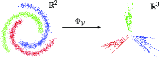
Figure 6: According to Theorem 2, the normalized Laplacian embedding of i.i.d. samples from a nonparametric mixture with small overlap, indivisible components and large enough sample size, has $(\alpha,\theta)$-OCS with $\alpha\ll 1$ and $\theta\ll 1$. The left plot shows i.i.d. samples in $\mathbb{R}^{2}$, and the right plot displays the image (in $\mathbb{R}^{3}$) of these data under the normalized Laplacian embedding, $\Phi_{\mathcal{V}}$. The embedding was performed using a regularized Gaussian kernel. The color of each point indicates the latent label of that point.

Theorem 2 establishes that the embedding of i.i.d. samples from a finite mixture ${\bar{\mathbb{P}}}$ has orthogonal cone structure (OCS) if the components have small overlap and good indivisibility. This result holds with high probability on the sampling from ${\bar{\mathbb{P}}}$. See Figure 6 for an illustration of the theorem.

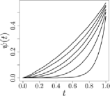
Figure 7: The tail decay function $\psi(t)$ roughly follows a power law for the standard Gaussian distribution and Gaussian kernel with bandwidths $\nu\in\{0.15,0.45,0.75,1,1.5,2.5\}$.

The tail decay of the mixture components enters the bounds on $\alpha$ and $\theta$ in different ways: the bound on $\theta$ is inversely proportional to $t$, but the bound on $\alpha$ is tighter for smaller $t$. Depending on how quickly $\psi$ increases with $t$, it may very well be the dominant term in the bound on $\alpha$. For example, if there is a $\gamma>0$ such that $\psi(t)\leq t^{\gamma}$ for all $t\in(0,1)$, and we set $t=\varphi_{n}^{\beta}$ for some $\beta\in(0,1)$, then we obtain the simplified bounds

$$|\cos\theta|\leq\frac{c}{w_{\min}^{3}}\varphi_{n}^{1/2-\beta}\quad\mbox{and}\quad\alpha\leq\frac{c}{(w_{\min})^{3/2}}\bigl{(}\varphi_{n}+\varphi_{n}^{\gamma\beta}\bigr{)}.$$

Indeed, we find that whenever $\gamma\beta<2$, the tail decay function is the dominant term in the bound on $\alpha$. Note that this power law tail decay is easy to verify for the Gaussian distribution with Gaussian kernel from Example 2; see Figure 7.

Finally, the numbers $c,c_{0},c_{1},c_{2}$ increase as the kernel bound $b$ increases and as $r$ decreases. This is where we need the tail truncation condition $r>0$. This assumption is common in the literature; see Cao and Chen compharmonic , for example. Both von Luxburg, Belkin and Bousquet luxburg and Rosasco, Belkin and De Vito rosasco assume $k(x,y)\geq r>0$, which is more restrictive. Note that this automatically holds if we add a positive constant to any kernel. This is sometimes called regularization and can significantly increase the performance of spectral clustering in practice chen .

3.4 Algorithmic consequences

In this section we apply our theory to study the performance of spectral clustering. The standard spectral clustering algorithm applies $K$-means to the embedded dataset. For completeness, we give pseudo code for the update step of $K$-means in Algorithm 1 below.

Algorithm 1 $K$-means update

Input: Normalized embedded data $y_{i}:=\frac{\Phi_{\mathcal{V}}(X_{i})}{\|\Phi_{\mathcal{V}}(X_{i})\|}$ for $i=1,\ldots,{n}$, and mean vectors $\{\mathbf{a}_{1},\ldots,\mathbf{a}_{K}\}$

for $m\in\{1,\ldots,K\}$ do

     

$${\hat{\mathcal{Z}}}_{m}\leftarrow\Bigl{\{}i\dvtx m=\operatorname{argmin}\limits_{\ell}\|{\mathbf{a}_{\ell}-y_{i}}\|\Bigr{\}}$$

     

$$\mathbf{a}^{\prime}_{m}\leftarrow\sum_{i\in{\hat{\mathcal{Z}}}_{m}}\frac{y_{i}}{|{\hat{\mathcal{Z}}}_{m}|}$$

end for

return $\{{\hat{\mathcal{Z}}}_{1},\ldots,{\hat{\mathcal{Z}}}_{K}\}$ and $\{{\mathbf{a}^{\prime}_{1}},\ldots,{\mathbf{a}^{\prime}_{K}}\}$

In practice, we have found that applying $K$-means to an embedded dataset works well if the underlying orthogonal cone structure is “nice enough.” The following proposition provides a quantitative characterization of this phenomenon. It applies to an embedded data set $\{\Phi_{\mathcal{V}}(X_{i}),{Z}_{i}\}_{i=1}^{n}$ with $(\alpha,\theta)$-OCS, and an initialization of $\mathbf{a}_{1},\ldots,\mathbf{a}_{K}$ as uniformly random orthonormal vectors. Recall the notation ${\mathcal{Z}}_{m}=\{i\in[{n}]|Z_{i}=m\}$.

Proposition 1

Suppose $\theta$ and $\alpha$ are sufficiently small that

$$\frac{\alpha{n}+(1-\alpha)|{\mathcal{Z}}_{m}|\sin\theta}{(1-\alpha)|{\mathcal{Z}}_{m}|} \leq \sin\frac{\pi}{8}\quad\mbox{and}$$

$$\frac{(1-\alpha)|{\mathcal{Z}}_{m}|\cos\theta-\alpha n}{|{\mathcal{Z}}_{m}|+\alpha n} \geq \frac{1}{2},\qquad m=1,\ldots,K.$$

Then there is a constant $c_{K}$ such that with probability at least $1-\frac{4c_{K}\theta}{2\pi}$ over the random initialization, the $K$-means algorithm misclusters at most $\alpha n$ points. When $K=2$, we have $c_{K}=1$.

Intuitively, condition (1) requires $\alpha$ and $\theta$ to be small enough so that the different cones from the $(\alpha,\theta)$-OCS do not overlap.

Proof of Proposition 1 We provide a detailed proof for the case $K=2$. By the definition of $(\theta,\alpha)$-OCS, there exist orthogonal vectors $e_{1},e_{2}$ such that a fraction $1-\alpha$ of the embedded samples with latent label $m$ lie within an angle $\theta$ of $e_{m}$, $m=1,2$. Let us say that the initialization is unfortunate if some $\mathbf{a}_{j}$ falls within angle $\frac{\theta}{2}$ of the angular bisector of $e_{1}$ and $e_{2}$, an event which occurs with probability $\frac{4\theta}{2\pi}$.

Suppose without loss of generality that $\mathbf{a}_{1}$ is closer to $e_{1}$, and let $\mathbf{a}^{\prime}_{1},\mathbf{a}^{\prime}_{2}$ denote the updates

$$\mathbf{a}^{\prime}_{m}=\sum_{i\in{\hat{\mathcal{Z}}}_{m}}\frac{v_{i}}{|{\hat{\mathcal{Z}}}_{m}|},\qquad m=1,2.$$

If the initialization is not unfortunate, then all points in the $\theta$-cone around $e_{1}$ are closer to $\mathbf{a}_{1}$ than $\mathbf{a}_{2}$. In this case, the $(\theta,\alpha)$-OCS implies that the $e_{2}$-coordinate of $\mathbf{a}^{\prime}_{1}$ is at most

$$\frac{\alpha{n}+(1-\alpha)|{\mathcal{Z}}_{1}|\sin\theta}{(1-\alpha)|{\mathcal{Z}}_{1}|}\leq\sin\frac{\pi}{8},$$

and the $e_{1}$-coordinate of $\mathbf{a}^{\prime}_{1}$ is at least

$$\frac{(1-\alpha)|{\mathcal{Z}}_{1}|\cos\theta-\alpha n}{|{\mathcal{Z}}_{1}|+\alpha n}\geq\frac{1}{2}.$$

We conclude that all points in the $\theta$-cone about $e_{1}$ are closer to ${\mathbf{a}^{\prime}_{1}}$ than ${\mathbf{a}^{\prime}_{2}}$. Consequently, we find that after a single update step of $K$-means, all but a fraction $\alpha$ of the samples are correctly labeled. Moreover, this holds for all subsequent $K$-means updates. This completes the proof for $K=2$.

The proof for general $K$ follows the same steps. The probability that any $\mathbf{a}_{m}$ falls within angle $\frac{\theta}{2}$ of the angular bisector of any pair $e_{j},e_{\ell}$ is still proportional to $\theta$, with a constant of proportionality $c_{K}$ that depends on $K$.

4 Proofs

We now turn to the proofs of our main results, beginning with the population level result stated in Theorem 1. We then provide the proof of Theorem 2 and Proposition 1.

4.1 Proof of Theorem 1

Our proof leverages an operator perturbation theorem due to Stewart stewart to show that ${\mathcal{Q}}$ is an approximate invariant subspace of the normalized Laplacian operator $\bar{\mathbf{T}}$ from equation (5). Recalling that ${\Pi_{{\mathcal{Q}}}}$ denotes the projection onto subspace ${\mathcal{Q}}$ (with ${\Pi_{{{\mathcal{Q}}^{\perp}}}}$ defined analogously), consider the following three operators:

$${\mathbf{A}}:={{\Pi_{{\mathcal{Q}}}}\bar{\mathbf{T}}{\Pi^{*}_{{\mathcal{Q}}}}},\qquad{\mathbf{B}}:={{\Pi_{{{\mathcal{Q}}^{\perp}}}}\bar{\mathbf{T}}{\Pi^{*}_{{{\mathcal{Q}}^{\perp}}}}}\quad\mbox{and}\quad{\mathbf{G}}:={{\Pi_{{{\mathcal{Q}}^{\perp}}}}\bar{\mathbf{T}}{\Pi^{*}_{{\mathcal{Q}}}}}.$$

By definition, a subspace ${\mathcal{Q}}$ is invariant under $\bar{\mathbf{T}}$ if and only if ${\mathbf{G}}=0$. In our setting, this ideal situation occurs when there is no overlap between mixture components. More generally, operator perturbation theory can be used to guarantee that a space is approximately invariant as long as the Hilbert–Schmidt norm ${|\!|\!|{\mathbf{G}}|\!|\!|_{\mathrm{HS}}}$ is not too large relative to the spectral separation between ${\mathbf{A}}$ and ${\mathbf{B}}$. In particular, define the quantities

$$\gamma:=|\!|\!|{\mathbf{G}}|\!|\!|_{\mathrm{HS}}\quad\mbox{and}\quad{\operatorname{sep}({\mathbf{A}},{\mathbf{B}})}:=\inf\bigl{\{}|a-b||a\in\sigma({\mathbf{A}}),b\in\sigma({\mathbf{B}})\bigr{\}}.$$

In application to our problem, Theorem 3.6 of Stewart stewart guarantees that as long as $\frac{\gamma}{{\operatorname{sep}({\mathbf{A}},{\mathbf{B}})}}<\frac{1}{2}$, then there is an operator ${\mathbf{S}}\dvtx{\mathcal{Q}}\rightarrow{{\mathcal{Q}}^{\perp}}$ such that

$$|\!|\!|{\mathbf{S}}|\!|\!|_{\mathrm{HS}} \leq \frac{2\gamma}{{\operatorname{sep}({\mathbf{A}},{\mathbf{B}})}}$$ (25)

such that ${\operatorname{Range}}({\Pi^{*}_{{\mathcal{Q}}}}+{\Pi^{*}_{{{\mathcal{Q}}^{\perp}}}}{\mathbf{S}})$ is an invariant subspace of $\bar{\mathbf{T}}$.

Accordingly, in order to apply this result, we first need to control the quantities $|\!|\!|{\mathbf{G}}|\!|\!|_{\mathrm{HS}}$ and ${\operatorname{sep}({\mathbf{A}},{\mathbf{B}})}$. The bulk of our technical effort is devoted to proving the following two lemmas:

Lemma 1 ((Hilbert–Schmidt bound))

We have

$${|\!|\!|{\mathbf{G}}|\!|\!|_{\mathrm{HS}}} \leq \frac{\sqrt{K(12+b_{\max})}}{w_{\min}}\sqrt{\mathcal{S}_{\max}({\bar{\mathbb{P}}})+{{\mathcal{C}}({\bar{\mathbb{P}}})}},$$ (26)

where $b_{\max}:=\max_{m=1,\ldots,K}{\|\int k_{m}(x,y)\,d\mathbb{P}_{m}(y)\|_{\infty}^{2}}$.

Lemma 2 ((Spectral separation bound))

Under the hypothesis of the theorem, we have

$$\sigma_{\min}({\mathbf{A}}) \geq 1-13K\bigl{[}\mathcal{S}_{\max}({\bar{\mathbb{P}}})+{{\mathcal{C}}({\bar{\mathbb{P}}})}\bigr{]}^{1/2}$$

and

$$\sigma_{\max}({\mathbf{B}}) \leq 1-\frac{\Gamma^{2}}{8}+\frac{3[{\mathcal{S}_{\max}({\bar{\mathbb{P}}})+{{\mathcal{C}}({\bar{\mathbb{P}}})}}]^{1/2}}{w_{\min}}.$$

Consequently, the spectral separation is lower bounded as

$${\operatorname{sep}({\mathbf{A}},{\mathbf{B}})} \geq \frac{\Gamma^{2}}{16}.$$ (28)

See Appendices A.1 and A.2 (supplementary material SchiebingerWainwrightYu14Sup ), respectively, for the proof of these lemmas.

Combined with our earlier bound (25), these two lemmas guarantee that

$${|\!|\!|{\mathbf{S}}|\!|\!|_{\mathrm{HS}}} \leq 16\sqrt{12+{b_{\max}}}\varphi({\bar{\mathbb{P}}},k).$$ (29)

Moreover, we find that ${\operatorname{Range}}({\Pi^{*}_{{\mathcal{Q}}}}+{\Pi^{*}_{{{\mathcal{Q}}^{\perp}}}}{\mathbf{S}})$ is equal to ${\mathcal{R}}$, the principal eigenspace of $\bar{\mathbf{T}}$. Indeed, by Stewart’s theorem, the spectrum of $\bar{\mathbf{T}}$ is the disjoint union $\sigma(\bar{\mathbf{T}})=\sigma({\mathbf{A}}+{\mathbf{G}}^{*}{\mathbf{S}})\cup\sigma({\mathbf{B}}-{\mathbf{S}}{\mathbf{G}}^{*})$. After some calculation using the upper bound on $\varphi({{\bar{\mathbb{P}}}},k)$ in the theorem hypothesis, we find that the spectrum of $\bar{\mathbf{T}}$ satisfies $\sigma_{\min}({\mathbf{A}}+{\mathbf{G}}^{*}{\mathbf{S}})>\sigma_{\max}({\mathbf{B}}-{\mathbf{S}}{\mathbf{G}}^{*})$, and any element $x\in{\operatorname{Range}}({\Pi^{*}_{{\mathcal{Q}}}}+{\Pi^{*}_{{{\mathcal{Q}}^{\perp}}}}{\mathbf{S}})$ must satisfy

$$\sup_{q\in{\mathcal{Q}}}\biggl{\{}\frac{x^{*}\bar{\mathbf{T}}x}{x^{*}x}\bigg{|}x=\bigl{(}{\Pi^{*}_{{\mathcal{Q}}}}+{\Pi^{*}_{{{\mathcal{Q}}^{\perp}}}}{\mathbf{S}}\bigr{)}q\biggr{\}}>\sigma_{\max}\bigl{(}{{\mathbf{B}}-{\mathbf{S}}{\mathbf{G}}^{*}}\bigr{)}.$$

Therefore ${\operatorname{Range}}({\Pi^{*}_{{\mathcal{Q}}}}+{\Pi^{*}_{{{\mathcal{Q}}^{\perp}}}}{\mathbf{S}})={\mathcal{R}}$.

The only remaining step is to translate bound (29) into a bound on the norm $|\!|\!|{\Pi_{{\mathcal{R}}}}-{\Pi_{{\mathcal{Q}}}}|\!|\!|_{\mathrm{HS}}$. Observe that the difference of projection operators can be written as

$${\Pi_{\mathcal{R}}}-{\Pi_{{\mathcal{Q}}}}=({\Pi_{\mathcal{R}}}+{\Pi_{\mathcal{R}^{\perp}}})({\Pi_{\mathcal{R}}}-{\Pi_{{\mathcal{Q}}}})={\Pi_{\mathcal{R}}}{\Pi_{{\mathcal{Q}}^{\perp}}}-{\Pi_{\mathcal{R}^{\perp}}}{\Pi_{{\mathcal{Q}}}}.$$

Now Lemma 3.2 of Stewart stewart gives the explicit representations

$$\Pi_{{\mathcal{R}}}=\bigl{(}{\mathbf{I}}+{\mathbf{S}}^{*}{\mathbf{S}}\bigr{)}^{-1/2}\bigl{(}{\Pi_{{\mathcal{Q}}}}+{\mathbf{S}}^{*}{\Pi_{{{\mathcal{Q}}^{\perp}}}}\bigr{)}$$

and

$$\Pi_{{\mathcal{R}}^{\perp}}=\bigl{(}{\mathbf{I}}+{\mathbf{S}}{\mathbf{S}}^{*}\bigr{)}^{-1/2}({\Pi_{{{\mathcal{Q}}^{\perp}}}}+{\Pi_{{\mathcal{Q}}}}{\mathbf{S}}).$$

Consequently, we have

$$|\!|\!|{\Pi_{\mathcal{R}^{\perp}}}{\Pi_{{\mathcal{Q}}}}|\!|\!|_{\mathrm{HS}}\leq\big{|}\!\big{|}\!\big{|}\bigl{(}{\mathbf{I}}+{\mathbf{S}}{\mathbf{S}}^{*}\bigr{)}^{-1/2}{\mathbf{S}}\big{|}\!\big{|}\!\big{|}_{\mathrm{HS}}$$

and

$$|\!|\!|{\Pi_{\mathcal{R}}}{\Pi_{{{\mathcal{Q}}^{\perp}}}}|\!|\!|_{\mathrm{HS}}\leq\big{|}\!\big{|}\!\big{|}\bigl{(}{\mathbf{I}}+{\mathbf{S}}^{*}{\mathbf{S}}\bigr{)}^{-1/2}{\mathbf{S}}^{*}\big{|}\!\big{|}\!\big{|}_{\mathrm{HS}}.$$

By the continuous functional calculus (see Section VII.1 of Reed and Simon reedsimon ), we have the expansion

$$\bigl{(}{\mathbf{I}}+{\mathbf{S}}{\mathbf{S}}^{*}\bigr{)}^{-1/2} = \sum_{n=1}^{\infty}\pmatrix{2n\cr n}\frac{({\mathbf{S}}{\mathbf{S}}^{*})^{n-1}}{2^{2n}}.$$

Putting together the pieces, in terms of the shorthand ${\varepsilon}={|\!|\!|{\mathbf{S}}|\!|\!|_{\mathrm{HS}}}$, we have

$$|\!|\!|{\Pi_{{\mathcal{R}}}}-{\Pi_{{\mathcal{Q}}}}|\!|\!|_{\mathrm{HS}} \leq \frac{{\varepsilon}}{2}\sum_{n=1}^{\infty}\pmatrix{2n\cr n}\biggl{(}\frac{{\varepsilon}}{2}\biggr{)}^{2(n-1)}=\frac{2}{{\varepsilon}}\biggl{(}\frac{1}{\sqrt{1-{\varepsilon}^{2}}}-1\biggr{)}\leq{\varepsilon},$$

which completes the proof.

4.2 Proof of Theorem 2

We say that a $K$-element subset (or $K$-tuple) of $\{X_{1},\ldots,X_{n}\}$ is diverse if the latent labels of all points in the subset are distinct. Given some $\theta\in(0,\frac{\pi}{4})$, a $K$-tuple is $\theta$-orthogonal if all its distinct pairs, when embedded, are orthogonal up to angle $\frac{\theta}{2}$. In order to establish $(\alpha,\theta)$-angular structure in the normalized Laplacian embedding of $\{X_{1},\ldots,X_{n}\}$, we must show that there is a subset of $\{X_{1},\ldots,X_{n}\}$ with at least $(1-\alpha){n}$ elements, and with the property that every diverse $K$-tuple from the subset is $\theta$-orthogonal.

We break the proof into two steps. We first lower bound the total number of $K$-tuples that are diverse and $\theta$-orthogonal. In the second step we construct the desired subset. We present the first step below and defer the second step to Appendix B.1 in the supplementary material SchiebingerWainwrightYu14Sup .

Step 1

Consider a diverse $K$-tuple $(X^{1},\ldots,X^{K})$ constructed randomly by selecting $X^{m}$ uniformly at random from the set $\{X_{i}|{Z}_{i}=m\}$ for $m=1,\ldots,K$. Form the $K\times K$ random matrix

$${V} = \left[\matrix{|&&|\cr\Phi_{\mathcal{V}}\bigl{(}X^{1}\bigr{)}&\cdots&\Phi_{\mathcal{V}}\bigl{(}X^{K}\bigr{)}\cr|&&|}\right],$$

where $\Phi_{\mathcal{V}}$ denotes the normalized Laplacian embedding from equation (3). Let ${\tilde{V}}$ denote an independent copy of ${V}$. Let ${Q}\in\mathbb{R}^{K\times K}$ denote the diagonal matrix with entries ${Q}_{mm}=\frac{q_{m}(X^{m})}{\|q_{m}\|_{{{\bar{\mathbb{P}}}_{n}}}}$, where ${\bar{\mathbb{P}}_{n}}$ is the empirical distribution over the samples $X_{1},\ldots,X_{n}$, and define $Q_{\max}:=\max_{m}\frac{{\|q_{m}\|_{\infty}}}{\|q_{m}\|_{\bar{\mathbb{P}}}}$.

At the core of our proof lies the following claim involving a constant $c_{3}$. For at least a fraction $1-\frac{2Kc_{3}\varphi_{n}(\delta)}{\sqrt{w_{\min}}}$ of the diverse $K$-tuples, we have the inequality

$$\big{|}\!\big{|}\!\big{|}{V^{T}}{\tilde{V}}-{Q}^{2}\big{|}\!\big{|}\!\big{|}_{\mathrm{HS}}\leq\frac{32\sqrt{3}}{w_{\min}^{3}}Q_{\max}^{2}\sqrt{c_{3}}\sqrt{\varphi_{n}(\delta)},$$ (30)

holding on a high probability set ${\mathcal{A}}$. For the moment, we take this claim as given, before returning to define ${\mathcal{A}}$ explicitly and prove the claim.

When inequality (30) is satisfied, we obtain the following upper bound on the off-diagonal elements of ${{{V}}^{T}}{\tilde{V}}$:

$$\bigl{(}{{{V}}^{T}}{\tilde{V}}\bigr{)}_{m\ell}\leq\frac{32\sqrt{3}Q_{\max}^{2}}{w_{\min}^{3}}\sqrt{c_{3}}\sqrt{\varphi_{n}(\delta)}\qquad\mbox{for }m\neq\ell.$$

This is useful because

$$\cos\operatorname{angle}\bigl{(}\Phi_{\mathcal{V}}\bigl{(}X^{m}\bigr{)},\Phi_{\mathcal{V}}\bigl{(}X^{\ell}\bigr{)}\bigr{)}=\frac{({{{V}}^{T}}{\tilde{V}})_{m\ell}}{\sqrt{({{{V}}^{T}}{V})_{mm}({{{V}}^{T}}{\tilde{V}})_{\ell\ell}}}.$$

However, we must also lower bound $\min_{m}({{{V}}^{T}}{\tilde{V}})_{mm}$. To this end, by union bound, we obtain

$$\Pr\Bigl{\{}\min_{m}{Q}_{mm}^{2}\leq t\Bigr{\}} = \Pr\biggl{\{}\min_{m}\frac{q_{m}^{2}(X^{m})}{{\|q_{m}\|^{2}_{{\bar{\mathbb{P}}_{n}}}}}\leq t\biggr{\}}$$

$$\leq \sum_{m=1}^{K}\Pr\biggl{\{}\frac{q_{m}^{2}(X^{m})}{{\|q_{m}\|^{2}_{{\bar{\mathbb{P}}_{n}}}}}\leq t\biggr{\}}$$

$$:= \psi_{n}(t).$$

On the set ${\mathcal{A}}_{\psi}:=\{\sup_{t}|\psi_{n}(t)-\psi(t)|\leq\delta\}\subset{\mathcal{A}}$, we may combine equations (30) and (4.2) to obtain

$$\min_{m}\bigl{(}{{{V}}^{T}}{\tilde{V}}\bigr{)}_{mm}\geq t-\frac{32\sqrt{3}Q_{\max}^{2}}{w_{\min}^{3}}\sqrt{c_{3}}\sqrt{\varphi_{n}(\delta)},$$

with probability at least $1-\psi(2t)$. Therefore, there is a $\theta$ satisfying

$$|\cos\theta|\leq\frac{32\sqrt{3}Q_{\max}^{2}\sqrt{c_{3}}\sqrt{\varphi_{n}(\delta)}}{w_{\min}^{3}t-32\sqrt{3}Q_{\max}^{2}\sqrt{c_{3}}\sqrt{\varphi_{n}(\delta)}}$$

such that at least a fraction $1-\frac{2Kc_{3}\varphi_{n}(\delta)}{\sqrt{w_{\min}}}-\psi(2t)$ of the diverse $K$-tuples are $\theta$-orthogonal on the set ${\mathcal{A}}$. This establishes the finite sample bound (23) with $c_{0}:=2c_{3}$ and $c_{1}:=32\sqrt{3}Q_{\max}^{2}\sqrt{c_{3}}$.

It remains to prove the intermediate claim (30). Define the matrix

$$A := \left[\matrix{\displaystyle\biggl{\langle}\frac{q_{1}}{\|q_{1}\|_{{{\bar{\mathbb{P}}}_{n}}}},v_{1}\biggr{\rangle}_{{\bar{\mathbb{P}}_{n}}}&\cdots&\displaystyle\biggl{\langle}\frac{q_{1}}{\|q_{1}\|_{{\bar{\mathbb{P}}_{n}}}},v_{K}\biggr{\rangle}_{{{\bar{\mathbb{P}}}_{n}}}\cr\vdots&\ddots&\vdots\cr\displaystyle\biggl{\langle}\frac{q_{K}}{\|q_{K}\|_{{{\bar{\mathbb{P}}}_{n}}}},v_{1}\biggr{\rangle}_{{\bar{\mathbb{P}}_{n}}}&\cdots&\displaystyle\biggl{\langle}\frac{q_{K}}{\|q_{K}\|_{{{\bar{\mathbb{P}}}_{n}}}},v_{K}\biggr{\rangle}_{{\bar{\mathbb{P}}_{n}}}}\right].$$ (32)

Note that the entries of $A{{A}^{T}}$ are

$$\bigl{(}A{{A}^{T}}\bigr{)}_{m\ell}=\frac{\langle{\Pi_{{\mathcal{V}}}}q_{m},{\Pi_{{\mathcal{V}}}}q_{\ell}\rangle_{{\bar{\mathbb{P}}_{n}}}}{\|q_{m}\|_{{\bar{\mathbb{P}}_{n}}}\|q_{\ell}\|_{{\bar{\mathbb{P}}_{n}}}}.$$

The off-diagonal elements satisfy

$$\bigl{(}A{{A}^{T}}\bigr{)}_{m\ell}\leq 3(\hat{\varphi}+\sqrt{\hat{\mathcal{S}}_{\max}})\qquad\mbox{for }m\neq\ell,$$

where $\hat{\varphi}=\max_{m}\frac{\|q_{m}-{\Pi_{{\mathcal{V}}}}q_{m}\|_{{\bar{\mathbb{P}}_{n}}}}{\|q_{m}\|_{{\bar{\mathbb{P}}_{n}}}}$, and $\hat{\mathcal{S}}_{\max}=\max_{m\neq\ell}\frac{{\|q_{\ell}\|^{2}_{\mathbb{P}_{m}^{n}}}}{{\|q_{m}\|^{2}_{{{\bar{\mathbb{P}}}_{n}}}}}$ (and $\mathbb{P}_{m}^{n}$ denotes the empirical distribution for the samples with latent label $m$). Similarly, the diagonal elements satisfy $|(A{{A}^{T}})_{mm}-1|\leq 3\hat{\varphi}$. Putting together the pieces yields ${|\!|\!|A{{A}^{T}}-I|\!|\!|_{\mathrm{HS}}}^{2}\leq 3K^{2}(\hat{\varphi}+\hat{\mathcal{S}}_{\max})$, which in turn implies

$$\big{|}\!\big{|}\!\big{|}{\bigl{(}A{{A}^{T}}\bigr{)}}^{-1}-I\big{|}\!\big{|}\!\big{|}_{\mathrm{HS}}^{2}\leq\frac{3K^{2}(\hat{\varphi}+\sqrt{\hat{\mathcal{S}}_{\max}})}{1-3K^{2}(\hat{\varphi}+\sqrt{\hat{\mathcal{S}}_{\max}})}.$$

We now transform this inequality into one involving ${{{V}}^{T}}{\tilde{V}}$. Write $B=A{V}$ and ${\tilde{B}}=A{\tilde{V}}$, and note that ${{{V}}^{T}}{\tilde{V}}={{B}^{T}}{(A{{A}^{T}})}^{-1}{\tilde{B}}$. Therefore, we find that

$$\big{|}\!\big{|}\!\big{|}{V^{T}}{\tilde{V}}-{Q}^{2}\big{|}\!\big{|}\!\big{|}_{\mathrm{HS}} \leq \big{|}\!\big{|}\!\big{|}{{B}^{T}}{\tilde{B}}-{Q}^{2}\big{|}\!\big{|}\!\big{|}_{\mathrm{HS}}+\big{|}\!\big{|}\!\big{|}{{B}^{T}}\bigl{[}{\bigl{(}A{{A}^{T}}\bigr{)}}^{-1}-I\bigr{]}{\tilde{B}}\big{|}\!\big{|}\!\big{|}_{\mathrm{HS}}$$

$$\leq 3|\!|\!|{Q}|\!|\!|_{\mathrm{HS}}|\!|\!|B-{Q}|\!|\!|_{\mathrm{HS}}+{|\!|\!|B|\!|\!|_{\mathrm{HS}}}^{2}\big{|}\!\big{|}\!\big{|}{\bigl{(}A{{A}^{T}}\bigr{)}}^{-1}-I\big{|}\!\big{|}\!\big{|}_{\mathrm{HS}},$$

where the last inequality used $|\!|\!|B|\!|\!|_{\mathrm{HS}}\leq 2|\!|\!|{Q}|\!|\!|_{\mathrm{HS}}$. Now note that the entries of $B$ are $B_{m\ell}=\frac{{\Pi_{{\mathcal{V}}}}q_{m}(X^{\ell})}{\|q_{m}\|_{{\bar{\mathbb{P}}_{n}}}}$. Therefore the difference $B-{Q}$ satisfies

$$\mathbb{E}\bigl{[}|\!|\!|B-{Q}|\!|\!|_{\mathrm{HS}}^{2}|X_{1},\ldots,X_{n}\bigr{]}\leq K^{2}\biggl{(}\frac{\hat{\varphi}}{\sqrt{{{\hat{w}}_{\min}}}}+\sqrt{\hat{\mathcal{S}}_{\max}}\biggr{)}^{2}+K\frac{\hat{\varphi}^{2}}{{{\hat{w}}_{\min}}},$$ (33)

where ${{\hat{w}}_{\min}}=\min_{m}\frac{{n}_{m}}{{n}}$, and the expectation above is over the selection of the random $K$-tuple $(X^{1},\ldots,X^{K})$.

Both $\hat{\mathcal{S}}_{\max}$ and $\hat{\varphi}$ are small with high probability. Indeed, Bernstein’s inequality guarantees that

$$\sqrt{\hat{\mathcal{S}}_{\max}}\leq\sqrt{\mathcal{S}_{\max}}+\delta$$ (34)

with probability at least $1-2K^{2}\exp{\frac{-{n}(\mathcal{S}_{\max}+\delta^{2})^{2}}{8Q_{\max}^{2}(2\mathcal{S}_{\max}+\delta^{2})}}$. We control $\hat{\varphi}$ with a finite sample version of Theorem 1, which we state as Proposition 2 below.

Let ${\mathcal{V}}=\operatorname{span}\{v_{1},\ldots,v_{K}\}$ denote the principal eigenspace of the normalized Laplacian matrix.

Proposition 2

There are constants ${c_{2}^{\prime}},c_{3}$ such that for any $\delta\in(0,\frac{\|k\|_{{\bar{\mathbb{P}}}}}{b\sqrt{2\pi}})$ satisfying condition (22), we have

$$\hat{\varphi}\leq c_{3}\varphi_{n}(\delta)$$ (35)

with probability at least $1-10K\exp({\frac{-{n}{c_{2}^{\prime}}\delta^{4}}{\delta^{2}+\mathcal{S}_{\max}({{\bar{\mathbb{P}}}})+{{\mathcal{C}}({\bar{\mathbb{P}}})}}})$.

See Section 4.3 for the proof of this auxiliary result.

On the set $\{\hat{\varphi}\leq c_{3}\varphi_{n}(\delta)\}\cap\{{{\hat{w}}_{\min}}\geq\frac{1}{2}w_{\min}\}:={\mathcal{A}}_{\zeta}\cap{\mathcal{A}}_{w}$, equation (33) simplifies to

$$\mathbb{E}\bigl{[}|\!|\!|B-{Q}|\!|\!|_{\mathrm{HS}}^{2}|X_{1},\ldots,X_{n}\bigr{]}\leq\frac{4K^{2}c_{3}^{2}\varphi_{n}^{2}(\delta)}{{w_{\min}}},$$

whenever $(\frac{\sqrt{2}c_{3}\varphi_{n}(\delta)}{\sqrt{w_{\min}}}+\mathcal{S}_{\max}+\delta)^{2}\leq\frac{3c_{3}^{2}\varphi_{n}^{2}(\delta)}{w_{\min}}$, which is a consequence of condition (22). By Markov’s inequality we obtain the following result: at least a fraction $1-\frac{2Kc_{3}\varphi_{n}(\delta)}{\sqrt{w_{\min}}}$ of the diverse $K$-tuples satisfies

$${|\!|\!|B-{Q}|\!|\!|_{\mathrm{HS}}}^{2}\leq\frac{2Kc_{3}\varphi_{n}}{\sqrt{w_{\min}}}.$$ (36)

For the diverse $K$-tuples that do satisfy inequality (36) we find that

$$\big{|}\!\big{|}\!\big{|}{{{V}}^{T}}{\tilde{V}}-{Q}^{2}\big{|}\!\big{|}\!\big{|}_{\mathrm{HS}}\leq\biggl{(}\frac{6\sqrt{2}K^{3/2}Q_{\max}}{w_{\min}^{1/4}}+32\sqrt{3}K^{3}Q_{\max}^{2}\biggr{)}\sqrt{c_{3}}{\sqrt{\varphi_{n}}},$$

valid on the set ${\mathcal{A}}={\mathcal{A}}_{w}\cap{\mathcal{A}}_{q}\cap{\mathcal{A}}_{\psi}\cap\{\hat{\varphi}\leq c_{3}\varphi_{n}(\delta)\}\cap\{\sqrt{\hat{\mathcal{S}}_{\max}}\leq\sqrt{\mathcal{S}_{\max}}+\delta\}$, thereby establishing the bound (30).

To complete the first step of the proof of Theorem 2, it remains to control the probability of ${\mathcal{A}}$. By Hoeffding’s inequality, we have ${\mathbb{P}}[{\mathcal{A}}_{w}]\geq 1-Ke^{{-{n}w_{\min}^{2}}/2}$. Finally, an application of Bernstein’s inequality controls the probability of ${{\mathcal{A}}_{q}}$, and an application of Glivenko–Cantelli controls the probability of ${{\mathcal{A}}_{\psi}}$. Putting together the pieces we find that ${\mathcal{A}}$ holds with probability at least $1-8K^{2}\exp({\frac{-{n}c_{2}\delta^{4}}{\delta^{2}+{\mathcal{S}}_{\max}({\bar{\mathbb{P}}})+{{\mathcal{C}}({\bar{\mathbb{P}}})}}})$, where $c_{2}:=\min({c_{2}^{\prime}},\frac{1}{8Q_{\max}^{2}})$.

4.3 Proof of Proposition 2

Consider the operator $\hat{\mathbf{T}}\dvtx{L^{2}({{\bar{\mathbb{P}}}_{n}})}\to{L^{2}({\bar{\mathbb{P}}_{n}})}$ defined by

$$(\hat{\mathbf{T}}f)(x)=\int\frac{1}{\bar{q}_{n}(x)}k(x,y)\frac{f(y)}{\bar{q}_{n}(y)}\,d{\bar{\mathbb{P}}_{n}}(y),$$

where $\bar{q}_{n}(x)=\frac{1}{{n}}\sum_{i=1}^{K}k(X_{i},x)$ is the square root kernelized density for the empirical distribution ${\bar{\mathbb{P}}_{n}}$ over the data $X_{1},\ldots,X_{n}$. ${\bar{k}}^{n}(x,y):=\frac{k(x,y)}{\bar{q}_{n}(x)\bar{q}_{n}(y)}$ for the normalized kernel function. Note that for any $f\in{L^{2}({\bar{\mathbb{P}}_{n}})}$ and $v\in\mathbb{R}^{n}$ with coordinates $v_{i}=f(X_{i})$, we have $(\hat{\mathbf{T}}f)(X_{j})=(Lv)_{j}$, where $L$ is the normalized Laplacian matrix (2). Consequently, the principal eigenspace ${\mathcal{V}}$ of $L$ is isomorphic to the principal eigenspace of $\hat{\mathbf{T}}$ which we also denote by ${\mathcal{V}}$ for simplicity.

To prove the proposition, we must relate $\hat{\mathbf{T}}$ to the normalized Laplacian operator $\bar{\mathbf{T}}$. These operators differ in both their measures of integration—namely, ${\bar{\mathbb{P}}_{n}}$ versus $\bar{\mathbb{P}}$—and their kernels, namely $\frac{k(x,y)}{\bar{q}_{n}(x)\bar{q}_{n}(y)}$ versus $\frac{k(x,y)}{\bar{q}(x)\bar{q}(y)}$. To bridge the gap we introduce an intermediate operator $\tilde{\mathbf{T}}\dvtx{L^{2}({{\bar{\mathbb{P}}}_{n}})}\to{L^{2}({\bar{\mathbb{P}}_{n}})}$ defined by

$$(\tilde{\mathbf{T}}f)(x)=\int\frac{1}{\bar{q}(x)}k(x,y)\frac{f(y)}{\bar{q}(y)}\,d{\bar{\mathbb{P}}_{n}}(y).$$

Let ${\tilde{\mathcal{V}}}$ denote the principal eigenspace of $\tilde{\mathbf{T}}$. The following lemma bounds the $\rho$-distance between the principal eigenspaces of $\tilde{\mathbf{T}}$ and $\hat{\mathbf{T}}$.

Lemma 3

For any $\delta\in[0,\frac{\|k\|_{{\bar{\mathbb{P}}}}}{b\sqrt{2\pi}}]$ satisfying condition (22), we have

$$\rho({\mathcal{V}},{\tilde{\mathcal{V}}})\leq\frac{{c_{4}}}{\Gamma^{2}}\biggl{(}\frac{1}{\sqrt{n}}+\delta\biggr{)},$$ (37)

with probability at least $1-4e^{-n\pi\delta^{2}/4}-2e^{-n\mathbf{E}\bar{k}\delta^{2}}$, where ${c_{4}}=1024\sqrt{2\pi K}\frac{\|k\|_{{\bar{\mathbb{P}}}}b}{r^{4}}$.

See Appendix B.3 (supplementary material SchiebingerWainwrightYu14Sup ) for a proof of this lemma.

We must upper bound $\|q_{m}-{\Pi_{{\mathcal{V}}}}q_{m}\|_{{\bar{\mathbb{P}}_{n}}}$. By the triangle inequality,

$$\|q_{m}-{\Pi_{{\mathcal{V}}}}q_{m}\|_{{{\bar{\mathbb{P}}}_{n}}} \leq \|q_{m}-{\Pi_{\mathcal{R}}}q_{m}\|_{{\bar{\mathbb{P}}_{n}}}+\|{\Pi_{\mathcal{R}}}q_{m}-{\Pi_{{\tilde{\mathcal{V}}}}}q_{m}\|_{{{\bar{\mathbb{P}}}_{n}}}$$

$${}+\|{\Pi_{{\mathcal{V}}}}q_{m}-{\Pi_{{\tilde{\mathcal{V}}}}}q_{m}\|_{{\bar{\mathbb{P}}_{n}}}.$$

Note that $\|{\Pi_{{\mathcal{V}}}}q_{m}-{\Pi_{{\tilde{\mathcal{V}}}}}q_{m}\|_{{\bar{\mathbb{P}}_{n}}}\leq\|q_{m}\|_{{\bar{\mathbb{P}}_{n}}}\rho({\tilde{\mathcal{V}}},{\mathcal{V}})$. We can control this term with the lemma. The term $\|q_{m}-{\Pi_{\mathcal{R}}}q_{m}\|_{{\bar{\mathbb{P}}_{n}}}$ is the empirical version of a quantity controlled by Theorem 1. We handle the empirical fluctuations with a version of Bernstein’s inequality. For $\delta_{p}\geq 0$ we have the inequality

$$\|q_{m}-{\Pi_{\mathcal{R}}}q_{m}\|_{{{\bar{\mathbb{P}}}_{n}}}\leq\|q_{m}-{\Pi_{\mathcal{R}}}q_{m}\|_{\bar{\mathbb{P}}}+\delta_{p}$$ (38)

with probability at least $1-2\exp(-\frac{n\delta_{p}^{4}}{8(\delta_{p}^{2}+{c_{\mathrm{pop}}}^{2}\varphi^{2})\tilde{Q}^{2}_{\max}})$, where

$$\tilde{Q}_{\max}=\max_{m}\frac{{\|q_{m}-{\Pi_{\mathcal{R}}}q_{m}\|_{\infty}}}{\|q_{m}\|_{\bar{\mathbb{P}}}}\quad\mbox{and}\quad c_{\mathrm{pop}}:=16\sqrt{12+\frac{b_{\max}}{K}}.$$

It remains to control $\|{\Pi_{\mathcal{R}}}q_{m}-{\Pi_{{\tilde{\mathcal{V}}}}}q_{m}\|_{{\bar{\mathbb{P}}_{n}}}$. Let ${\bar{\mathcal{H}}}$ denote the reproducing kernel Hilbert space (RKHS) for the kernel ${\bar{k}}$. Now we define two integral operators on ${\bar{\mathcal{H}}}$. Let $\bar{\mathbf{H}}$ denote the operator defined by

$$(\bar{\mathbf{H}}h)(x)=\int{\bar{k}}(x,y)h(y)\,d\bar{\mathbb{P}}(y),$$

and similarly let $\tilde{\mathbf{H}}\dvtx{\bar{\mathcal{H}}}\to{\bar{\mathcal{H}}}$ denote the operator defined by

$$(\tilde{\mathbf{H}}h)(x)=\int{\bar{k}}(x,y)h(y)\,d{{\bar{\mathbb{P}}}_{n}}(y).$$

Both $\bar{\mathbf{H}}$ and $\tilde{\mathbf{H}}$ are self-adjoint, compact operators on ${\bar{\mathcal{H}}}$ and have real, discrete spectra. Let ${\mathcal{G}}$ denote the principal $K$-dimensional eigenspace of $\bar{\mathbf{H}}$, and let ${\tilde{\mathcal{G}}}$ denote the principal $K$-dimensional principal eigenspace of $\tilde{\mathbf{H}}$. The following lemma bounds the $\rho$-distance between these subspaces of ${\bar{\mathcal{H}}}$.

Lemma 4

For any $\delta>0$ satisfying condition (22), we have

$$\rho({\mathcal{G}},{\tilde{\mathcal{G}}})\leq\frac{c_{5}}{\Gamma^{2}}\biggl{(}\frac{1}{\sqrt{n}}+\delta\biggr{)}$$

with probability at least $1-2e^{-{n}\pi\mathbb{E}{\bar{k}}({\bar{X}},{\bar{X}})\delta^{2}}$, where $c_{5}=64\sqrt{2\pi K}\sqrt{\mathbb{E}{\bar{k}}({\bar{X}},{\bar{X}})}\frac{b}{r^{2}}$.

See Appendix B.2 (supplementary material SchiebingerWainwrightYu14Sup ) for the proof of this lemma.

By the triangle inequality, we have

$$\|{\Pi_{\mathcal{R}}}q_{m}-{\Pi_{{\tilde{\mathcal{V}}}}}q_{m}\|_{{\bar{\mathbb{P}}_{n}}} \leq \|{\Pi_{\mathcal{R}}}q_{m}-{\Pi_{{\mathcal{G}}}}q_{m}\|_{{\bar{\mathbb{P}}_{n}}}+\|{\Pi_{{\mathcal{G}}}}q_{m}-{\Pi_{{\tilde{\mathcal{G}}}}}q_{m}\|_{{\bar{\mathbb{P}}_{n}}}$$

$${}+\|{\Pi_{{\tilde{\mathcal{G}}}}}q_{m}-{\Pi_{{\tilde{\mathcal{V}}}}}q_{m}\|_{{\bar{\mathbb{P}}_{n}}}.$$

We claim that

$$\|{\Pi_{\mathcal{R}}}q_{m}-{\Pi_{{\mathcal{G}}}}q_{m}\|_{{\bar{\mathbb{P}}_{n}}}=0\quad\mbox{and}\quad\|{\Pi_{{\tilde{\mathcal{G}}}}}q_{m}-{\Pi_{{\tilde{\mathcal{V}}}}}q_{m}\|_{{\bar{\mathbb{P}}_{n}}}=0.$$ (39)

We take these identities as given for the moment, before returning to prove them at the end of this subsection.

Now the term $\|{\Pi_{{\mathcal{G}}}}q_{m}-{\Pi_{{\tilde{\mathcal{G}}}}}q_{m}\|_{{\bar{\mathbb{P}}_{n}}}$ can be controlled using the lemma in the following way. For any $h\in{\bar{\mathcal{H}}}$, note that

$$\|h\|_{{\bar{\mathbb{P}}_{n}}}^{2}=\frac{1}{n}\sum_{i=1}^{n}\langle h,{\bar{k}}_{X_{i}}\rangle_{{\bar{\mathcal{H}}}}^{2}\leq\frac{1}{n}\sum_{i=1}^{n}\|h\|_{\bar{\mathcal{H}}}^{2}{\bar{k}}(X_{i},X_{i})$$

by Cauchy–Schwarz for the RKHS inner product. Using this logic with $h={\Pi_{{\mathcal{G}}}}q_{m}-{\Pi_{{\tilde{\mathcal{G}}}}}q_{m}$, we find

$$\|{\Pi_{{\mathcal{G}}}}q_{m}-{\Pi_{{\tilde{\mathcal{G}}}}}q_{m}\|_{{\bar{\mathbb{P}}_{n}}}\leq\|q_{m}\|_{\bar{\mathcal{H}}}\sqrt{\frac{1}{n}\sum_{i=1}^{n}{\bar{k}}(X_{i},X_{i})}\rho({\mathcal{G}},{\tilde{\mathcal{G}}}).$$ (40)

Collecting our results and applying Lemmas 3 and 4 yields

$$\|q_{m}-{\Pi_{{\mathcal{V}}}}q_{m}\|_{{{\bar{\mathbb{P}}}_{n}}}\leq(c_{\mathrm{pop}}\varphi+\delta_{p}){\|q_{m}\|_{\bar{\mathbb{P}}}}+\frac{c_{n}\|q_{m}\|_{{{\bar{\mathbb{P}}}_{n}}}}{\Gamma^{2}}\biggl{(}\frac{1}{\sqrt{n}}+\delta\biggr{)},$$

where

$$c_{n} := \frac{256\sqrt{2\pi K}b}{r^{2}}\biggl{[}\frac{\|q_{m}\|_{\bar{\mathcal{H}}}}{\|q_{m}\|_{\bar{\mathbb{P}}}}\mathbb{E}{\bar{k}}({\bar{X}},{\bar{X}})+\frac{2b}{r^{2}}\biggr{]}.$$ (41)

By an application of Bernstein’s inequality, we have

$$\|q_{m}\|_{{\bar{\mathbb{P}}_{n}}}\leq\sqrt{2}\|q_{m}\|_{\bar{\mathbb{P}}}$$

with probability at least $1-2e^{{-{n}}/(16Q_{\max}^{2})}$. For $\delta\in(0,\frac{1}{2\sqrt{2\pi}Q_{\max}})$, we have

$$2e^{(-{n}{c_{\mathrm{pop}}}^{2}\delta^{4})/(8\Gamma^{4}\tilde{Q}_{\max}^{2}(\delta^{2}+\mathcal{S}_{\max}({{\bar{\mathbb{P}}}})+{{\mathcal{C}}({\bar{\mathbb{P}}})}))}+6e^{-{n}\pi\delta^{2}/2}+2e^{-{n}/(16Q_{\max}^{2})}$$

$$\qquad\leq 10e^{-({n{c_{2}^{\prime}}\delta^{4}})/({\delta^{2}+\mathcal{S}_{\max}({\bar{\mathbb{P}}})+{{\mathcal{C}}({\bar{\mathbb{P}}})}})},$$

where $\delta_{p}=\frac{c_{\mathrm{pop}}\delta}{\Gamma^{2}}$, and ${c_{2}^{\prime}}=\min(\frac{c_{\mathrm{pop}}^{2}}{8\Gamma^{4}\tilde{Q}_{\max}^{2}},\frac{\pi}{2})$. Modulo the claim, this proves the proposition with $c_{3}=2\max(c_{\mathrm{pop}},c_{n})$.

We now return to prove claim (39). Note the following relation between the eigenfunctions of $\bar{\mathbf{T}}$ and those of $\bar{\mathbf{H}}$: if $r_{i}$ is an eigenfunction of $\bar{\mathbf{T}}$ with eigenvalue $\lambda_{i}$ and $\|r_{i}\|_{{\bar{\mathbb{P}}}}=1$, then $g_{i}:={\sqrt{\lambda_{i}}}r_{i}$ has unit norm in ${\bar{\mathcal{H}}}$ and is an eigenfunction of $\bar{\mathbf{H}}$ with eigenvalue $\lambda_{i}$. Note that the eigenfunctions $r_{i}$ of $\bar{\mathbf{T}}$ form an orthonormal basis of ${L^{2}({\bar{\mathbb{P}}})}$, and therefore $q_{m}=\sum_{i=1}^{\infty}a_{i}r_{i}$, where $a_{i}$ are the coefficients $\langle q_{m},r_{i}\rangle_{\bar{\mathbb{P}}}$. By the observation above, we have the equivalent representation $q_{m}=\sum_{i=1}^{\infty}\frac{a_{i}}{\sqrt{\lambda_{i}}}g_{i}$. Therefore the ${L^{2}(\bar{\mathbb{P}})}$ projection onto $\mathcal{R}=\operatorname{span}\{r_{1},\ldots,r_{K}\}$ is ${\Pi_{\mathcal{R}}}q_{m}=\sum_{i=1}^{K}a_{i}r_{i}$, and the ${\bar{\mathcal{H}}}$ projection onto ${\mathcal{G}}=\operatorname{span}\{g_{1},\ldots,g_{K}\}$ is ${\Pi_{{\mathcal{G}}}}q_{m}=\sum_{i=1}^{K}\frac{a_{i}}{\sqrt{\lambda_{i}}}g_{i}$. Therefore the relation $g_{i}={\sqrt{\lambda_{i}}}r_{i}$ implies $\|{\Pi_{\mathcal{R}}}-{\Pi_{{\mathcal{G}}}}\|_{{\bar{\mathbb{P}}_{n}}}=0$. Similar reasoning yields $\|{\Pi_{{\tilde{\mathcal{G}}}}}q_{\ell}-{\Pi_{{\tilde{\mathcal{V}}}}}q_{\ell}\|_{{\bar{\mathbb{P}}_{n}}}=0$.

5 Discussion

In this paper, we have analyzed the performance of spectral clustering in the context of nonparametric finite mixture models. Our first main contribution is an upper bound on the distance between the population level normalized Laplacian embedding and the square root kernelized density embedding. This bound depends on the maximal similarity index, the coupling parameter, and the indivisibility parameter. These parameters all depend on the kernel function, and we present our analysis for a fixed but arbitrary kernel.

Although this dependence on the kernel function might seem undesirable, it is actually necessary to guarantee identifiability of the mixture components in the following sense. A mixture with fully nonparametric components is a very rich model class: without any restrictions on the mixture components, any distribution can be written as a $K$-component mixture in uncountably many ways. Conversely, when the clustering difficulty function is zero, the representation of a distribution as a mixture is unique. In principle, one could optimize over the convex cone of symmetric positive definite kernel functions so to minimize our clustering difficulty parameter. In our preliminary numerical experiments, we have found promising results in using this strategy to choose the bandwidth in a family of kernels.

Building on our population-level result, we have also provided a result that characterizes the normalized Laplacian embedding when applied to a finite collection of $n$ i.i.d. samples. We find that when the clustering difficulty is small, the embedded samples take on approximate orthogonal structure: samples from different components are almost orthogonal with high probability. The emergence of this form of angular structure allows an angular version of $K$-means to correctly label most of the samples.

Perhaps surprising is the fact that the optimal bandwidth (minimizing our upper bound) is nonzero. Although we only provide an upper bound, we believe this is fundamental to spectral clustering, not an artifact of our analysis. Again, the principal $K$-dimensional eigenspace of the Laplacian operator is not a well-defined mathematical object when the bandwidth is zero. Indeed, as the bandwidth shrinks to zero, the eigengap distinguishing this eigenspace from the remaining eigenfucntion vanishes. This eigenspace, however, is the population-level version of the subspace onto which spectral clustering projects. For this reason, we caution against shrinking the bandwidth indefinitely to zero, and we conjecture that there is an optimal population level bandwidth for spectral clustering. However, we should mention that we cannot provably rule out the optimality of an appropriately slowly shrinking bandwidth, and we leave this to future work. Further investigation of kernel bandwidth selection for spectral clustering is an interesting avenue for future work.

References

- (1) {barticle}[mr] \bauthor\bsnmAmini, \bfnmArash A.\binitsA. A., \bauthor\bsnmChen, \bfnmAiyou\binitsA., \bauthor\bsnmBickel, \bfnmPeter J.\binitsP. J. and \bauthor\bsnmLevina, \bfnmElizaveta\binitsE. (\byear2013). \btitlePseudo-likelihood methods for community detection in large sparse networks. \bjournalAnn. Statist. \bvolume41 \bpages2097–2122. \biddoi=10.1214/13-AOS1138, issn=0090-5364, mr=3127859 \bptokimsref\endbibitem
- (2) {barticle}[auto:parserefs-M02] \bauthor\bsnmBelkin, \bfnmM.\binitsM. and \bauthor\bsnmNiyogi, \bfnmP.\binitsP. (\byear2003). \btitleLaplacian eigenmaps for dimensionality reduction and data representation. \bjournalNeural Comput. \bvolume15 \bpages1373–1396. \bptokimsref\endbibitem
- (3) {barticle}[mr] \bauthor\bsnmCao, \bfnmYing\binitsY. and \bauthor\bsnmChen, \bfnmDi-Rong\binitsD.-R. (\byear2011). \btitleConsistency of regularized spectral clustering. \bjournalAppl. Comput. Harmon. Anal. \bvolume30 \bpages319–336. \biddoi=10.1016/j.acha.2010.09.002, issn=1063-5203, mr=2784567 \bptokimsref\endbibitem
- (4) {barticle}[mr] \bauthor\bsnmDonath, \bfnmW. E.\binitsW. E. and \bauthor\bsnmHoffman, \bfnmA. J.\binitsA. J. (\byear1973). \btitleLower bounds for the partitioning of graphs. \bjournalIBM J. Res. Develop. \bvolume17 \bpages420–425. \bidissn=0018-8646, mr=0329965 \bptokimsref\endbibitem
- (5) {barticle}[mr] \bauthor\bsnmFiedler, \bfnmMiroslav\binitsM. (\byear1973). \btitleAlgebraic connectivity of graphs. \bjournalCzechoslovak Math. J. \bvolume23 \bpages298–305. \bidissn=0011-4642, mr=0318007 \bptokimsref\endbibitem
- (6) {bincollection}[mr] \bauthor\bsnmGiné, \bfnmEvarist\binitsE. and \bauthor\bsnmKoltchinskii, \bfnmVladimir\binitsV. (\byear2006). \btitleEmpirical graph Laplacian approximation of Laplace–Beltrami operators: Large sample results. In \bbooktitleHigh Dimensional Probability. \bseriesInstitute of Mathematical Statistics Lecture Notes—Monograph Series \bvolume51 \bpages238–259. \bpublisherIMS, \blocationBeachwood, OH. \biddoi=10.1214/074921706000000888, mr=2387773 \bptokimsref\endbibitem
- (7) {barticle}[auto:parserefs-M02] \bauthor\bsnmJenssen, \bfnmR.\binitsR. (\byear2010). \btitleKernel entropy component analysis. \bjournalIEEE Trans. Pattern Anal. Mach. Intell. \bvolume32 \bpages847–860. \bptokimsref\endbibitem
- (8) {barticle}[mr] \bauthor\bsnmLawler, \bfnmGregory F.\binitsG. F. and \bauthor\bsnmSokal, \bfnmAlan D.\binitsA. D. (\byear1988). \btitleBounds on the spectrum for Markov chains and Markov processes: A generalization of Cheeger’s inequality. \bjournalTrans. Amer. Math. Soc. \bvolume309 \bpages557–580. \biddoi=10.2307/2000925, issn=0002-9947, mr=0930082 \bptokimsref\endbibitem
- (9) {bincollection}[auto:parserefs-M02] \bauthor\bsnmMeila, \bfnmM.\binitsM. and \bauthor\bsnmShi, \bfnmJ.\binitsJ. (\byear2001). \btitleA random walks view of spectral segmentation. In \bbooktitleProceedings of the Eighth International Workshop on Artificial Intelligence and Statistics, \blocationKey West, FL. \bptokimsref\endbibitem
- (10) {bincollection}[auto:parserefs-M02] \bauthor\bsnmNg, \bfnmA. Y.\binitsA. Y., \bauthor\bsnmJordan, \bfnmM. I.\binitsM. I. and \bauthor\bsnmWeiss, \bfnmY.\binitsY. (\byear2001). \btitleOn spectral clustering: Analysis and an algorithm. In \bbooktitleAdvances in Neural Information Processing Systems (NIPS), \blocationVancouver, BC, Canada. \bptokimsref\endbibitem
- (11) {bbook}[mr] \bauthor\bsnmReed, \bfnmMichael\binitsM. and \bauthor\bsnmSimon, \bfnmBarry\binitsB. (\byear1980). \btitleMethods of Modern Mathematical Physics. I: Functional Analysis, \bedition2nd ed. \bpublisherAcademic Press, \blocationNew York. \bidmr=0751959 \bptokimsref\endbibitem
- (12) {barticle}[mr] \bauthor\bsnmRosasco, \bfnmLorenzo\binitsL., \bauthor\bsnmBelkin, \bfnmMikhail\binitsM. and \bauthor\bsnmDe Vito, \bfnmErnesto\binitsE. (\byear2010). \btitleOn learning with integral operators. \bjournalJ. Mach. Learn. Res. \bvolume11 \bpages905–934. \bidissn=1532-4435, mr=2600634 \bptokimsref\endbibitem
- (13) {bmisc}[author] \bauthor\bsnmSchiebinger, \bfnmG.\binitsG., \bauthor\bsnmWainwright, \bfnmM. J.\binitsM. J. and \bauthor\bsnmYu, \bfnmB.\binitsB. (\byear2015). \bhowpublishedSupplement to “The geometry of kernelized spectral clustering.” DOI:\doiurl10.1214/14-AOS1283SUPP. \bptokimsref \bptokimsref\endbibitem
- (14) {barticle}[auto:parserefs-M02] \bauthor\bsnmShi, \bfnmJ.\binitsJ. and \bauthor\bsnmMalik, \bfnmJ.\binitsJ. (\byear2000). \btitleNormalized cuts and image segmentation. \bjournalIEEE Trans. Pattern Anal. Mach. Intell. \bvolume22 \bpages888–905. \bptokimsref\endbibitem
- (15) {barticle}[mr] \bauthor\bsnmShi, \bfnmTao\binitsT., \bauthor\bsnmBelkin, \bfnmMikhail\binitsM. and \bauthor\bsnmYu, \bfnmBin\binitsB. (\byear2009). \btitleData spectroscopy: Eigenspaces of convolution operators and clustering. \bjournalAnn. Statist. \bvolume37 \bpages3960–3984. \biddoi=10.1214/09-AOS700, issn=0090-5364, mr=2572449 \bptokimsref\endbibitem
- (16) {barticle}[mr] \bauthor\bsnmStewart, \bfnmG. W.\binitsG. W. (\byear1971). \btitleError bounds for approximate invariant subspaces of closed linear operators. \bjournalSIAM J. Numer. Anal. \bvolume8 \bpages796–808. \bidissn=0036-1429, mr=0293831 \bptokimsref\endbibitem
- (17) {barticle}[mr] \bauthor\bparticlevon \bsnmLuxburg, \bfnmUlrike\binitsU., \bauthor\bsnmBelkin, \bfnmMikhail\binitsM. and \bauthor\bsnmBousquet, \bfnmOlivier\binitsO. (\byear2008). \btitleConsistency of spectral clustering. \bjournalAnn. Statist. \bvolume36 \bpages555–586. \biddoi=10.1214/009053607000000640, issn=0090-5364, mr=2396807 \bptokimsref\endbibitem
- (18) {barticle}[mr] \bauthor\bsnmYan, \bfnmDonghui\binitsD., \bauthor\bsnmChen, \bfnmAiyou\binitsA. and \bauthor\bsnmJordan, \bfnmMichael I.\binitsM. I. (\byear2013). \btitleCluster forests. \bjournalComput. Statist. Data Anal. \bvolume66 \bpages178–192. \biddoi=10.1016/j.csda.2013.04.010, issn=0167-9473, mr=3064033 \bptokimsref\endbibitem