The Synchrosqueezing transform for instantaneous spectral analysis

Abstract

The Synchrosqueezing transform is a time-frequency analysis method that can decompose complex signals into time-varying oscillatory components. It is a form of time-frequency reassignment that is both sparse and invertible, allowing for the recovery of the signal. This article presents an overview of the theory and stability properties of Synchrosqueezing, as well as applications of the technique to topics in cardiology, climate science and economics.

1 Introduction

The Synchrosqueezing transform is a time-frequency analysis method that can characterize signals with time-varying oscillatory properties. It is designed to analyze and decompose signals of the form

$$f(t)=\sum_{k=1}^{K}A_{k}(t)e^{2\pi i\phi_{k}(t)},$$ (1)

where the $A_{k}$ and $\phi_{k}$ are time-varying amplitude and phase functions respectively. The goal is to recover the instantaneous frequencies (IFs) $\{\phi_{k}^{\prime}\}_{1\leq k\leq K}$ and the oscillatory components $\{A_{k}e^{2\pi i\phi_{k}}\}_{1\leq k\leq K}$. Signals of the form (1) arise in numerous scientific and engineering applications but are not well represented in a traditional Fourier basis, where the individual elements of the basis fail to capture localized oscillations in the components $\{A_{k}e^{2\pi i\phi_{k}}\}$. Standard time-frequency methods such as the short-time Fourier transform (STFT) and the continuous wavelet transform (CWT) are often used to analyze such signals, but do not take advantage of any sparsity of the form (1) in the signal and incur a tradeoff in time-frequency resolution [5, 8]. Synchrosqueezing is a variant of time-frequency reassignment (TFR), a class of techniques that apply a nonlinear post-processing mapping to a conventional STFT or CWT plot. The mapping is designed to “push” the energy in an STFT closer to its most prominent frequencies, resulting in a sparse and concentrated time-frequency representation of the signal [2, 9]. However, traditional TFR methods result in a loss of information from the underlying transform and cannot be used to recover the original signal, and also often involve heuristics that are difficult to justify rigorously.

Synchrosqueezing combines the localization and sparsity properties of TFR with the invertibility of a traditional time-frequency transform, and is robust to a variety of disturbances in the signal. The main concepts behind Synchrosqueezing were originally introduced in the mid-1990s for audio signal analysis [7], but it has received much closer attention in recent years, with an extensive mathematical theory developed in [6] and [15]. Unlike traditional TFR, Synchrosqueezing performs the post-processing mapping only in the frequency direction and does so in a manner that preserves the total energy of the signal $f$, allowing for the decomposition of the signal into the components $\{A_{k}e^{2\pi i\phi_{k}}\}$. This article provides a concise survey of the Synchrosqueezing methodology and its associated theory, and also discusses real-world applications in several different domains where the technique has provided new insights.

2 The Synchrosqueezing process

The Synchrosqueezing transform was originally developed in [6] and [7] in terms of the CWT. We choose a (complex) mother wavelet $\psi$ such that the Fourier transform $\hat{\psi}$ has strictly positive support and satisfies the standard admissibility condition $\int_{0}^{\infty}z^{-1}\hat{\psi}(z)dz<\infty$ [5]. The CWT $W_{\psi}f(a,t)$ at the scale $a$ and time shift $t$ is then given by

$$W_{\psi}f(a,t)=a^{-1/2}\int_{-\infty}^{\infty}f(u)\overline{\psi\left(\frac{u-t}{a}\right)}du.$$ (2)

We then take the phase transform $\omega f(a,b)$, defined as the derivative of the complex phase of $W_{\psi}f$,

$$\omega f(a,t)=\frac{\frac{\partial}{\partial t}W_{\psi}f(a,t)}{2\pi iW_{\psi}f(a,t)}.$$ (3)

Intuitively, this nonlinear operator can be thought of as removing the influence of $\psi$ from the CWT and “encoding” the localized frequency information we want. The key step is to consider the CWT Synchrosqueezing transform,

$$S_{\epsilon}^{\delta,M}f(t,\eta)=\int_{\{(a,t):a\in[M^{-1},M],|W_{\psi}f(a,t)|>\epsilon\}}a^{-3/2}W_{\psi}f(a,t)\frac{1}{\delta}h\left(\frac{\eta-\omega f(a,t)}{\delta}\right)da$$ (4)

for a test function $h\in C_{0}^{\infty}$, a sufficiently large parameter $M$, and sufficiently small $\delta>0$ and $\epsilon>0$. The motivation for (4) is that it is a smoothed out approximation to

$$Sf(t,\eta)=\int_{\{(a,t):\eta=\omega f(a,t)\}}a^{-3/2}W_{\psi}f(a,t)da,$$

or in other words, a partial inversion of the CWT that is only taken over the level curves of the phase transform $\omega f$ and ignores the rest of the time-scale plane $(a,t)$. This localization process allows us to recover the components $A_{k}e^{2\pi i\phi_{k}}$ more accurately than inverting the CWT over the entire time-scale plane. Alternatively, the mapping $W_{\psi}f(a,t)\to Sf(t,\eta)$ can be thought of as a reassignment operation that squeezes energy from the scales $a$ into IFs $\eta$ centered on the level curves of $\omega f$, but leaves the total energy in $W_{\psi}f(a,t)$ at each time $t$ unchanged. For appropriate signals $f$, the energy in the Synchrosqueezing transform $S_{\epsilon}^{\delta,M}f(b,\eta)$ is concentrated precisely around the IF curves $\{\phi_{k}^{\prime}(t)\}$. Finally, once $S_{\epsilon}^{\delta,M}f$ is computed, we can recover each of the components by completing the inversion of the CWT and integrating over small bands around each IF curve,

$$R_{k,\epsilon}^{\delta,M}f(t)=\frac{1}{\int_{0}^{\infty}\frac{\hat{\psi}(z)}{z}dz}\int_{|\eta-\phi_{k}^{\prime}(t)|<\epsilon}S_{\epsilon}^{\delta,M}f(t,\eta)d\eta.$$ (5)

Under certain conditions, it can be shown that $R_{k,\epsilon}^{\delta,M}f(t)\approx A_{k}(t)e^{2\pi i\phi_{k}(t)}$. In practice, an additional, intermediate step is needed to identify the integration bands in (5), which is typically accomplished by a ridge extraction method that determines the maxima in the time-frequency plot $|S_{\epsilon}^{\delta,M}f(t,\eta)|$. A discretized formulation of the steps (2)-(5) and related computational details can be found in [14].

The main concepts behind Synchrosqueezing can also be applied to other underlying time-frequency representations. The paper [15] develops a parallel approach based on the short-time Fourier transform (STFT), which is shown to have some advantages. The STFT Synchrosqueezing process is similar to the above development, but instead of (2) is based on the modified STFT for an appropriate window function $G$,

$$V_{G}f(t,z)=\int_{-\infty}^{\infty}f(u)G(u-t)e^{-2\pi iz(u-t)}du.$$ (6)

This is simply the standard STFT with an additional modulation factor $e^{2\pi izt}$, and can be thought of as a filter bank taken by sliding the window $G$ over different frequency bands. The phase transform (3) and Synchrosqueezing transform (4) respectively become

$$\tilde{\omega}f(z,t)=\frac{\frac{\partial}{\partial t}V_{G}f(t,z)}{2\pi iV_{G}f(t,z)},$$

$$\tilde{S}_{\epsilon}^{\delta,M}f(t,\eta)=\int_{\{(t,z):z\in[M^{-1},M],|V_{G}f(t,\eta)|>\epsilon\}}V_{G}f(t,z)\frac{1}{\delta}h\left(\frac{\eta-\tilde{\omega}f(t,z)}{\delta}\right)dz,$$ (7)

and the components can be recovered by fully inverting (7) as before by taking

$$\tilde{R}_{k,\epsilon}^{\delta,M}f(t)=\frac{1}{\int_{-\infty}^{\infty}|G(z)|^{2}dz}\int_{|\eta-\phi_{k}^{\prime}|<\epsilon}\tilde{S}_{\epsilon}^{\delta,M}f(t,\eta)d\eta.$$ (8)

A simple example of the time-frequency plots $|S_{\epsilon}^{\delta,M}(t,\eta)|$ and $|\tilde{S}_{\epsilon}^{\delta,M}f(t,\eta)|$ is shown in Figure 1. While the traditional STFT and CWT plots are blurry, reflecting the fact that they are not sparse representations of the signal, the Synchrosqueezing transforms have a much more concentrated profile and distinct IF curves in the time-frequency plane. Several additional examples can be found in [14], comparing CWT Synchrosqueezing with TFR methods and other techniques. An open source MATLAB toolbox implementing both forms of Synchrosqueezing is available [3] and has facilitated the use of the technique across different disciplines.

We briefly describe several extensions of these concepts that have been developed. The paper [16] considers a variant of the signal model in (1), where the mode $A_{k}(t)e^{2\pi i\phi_{k}(t)}$ is replaced by a more general form $A_{k}(t)s(\phi_{k}(t))$ for a given “shape function” $s$ chosen to fit a particular application at hand. This turns out to be a natural model for the analysis of electrocardiogram signals, in which the sharp spikes (see Figure 2) are not well represented by standard Fourier harmonics. In [12], another generalization is presented based on replacing (6) with a “generalized Fourier transform,” i.e an oscillatory integral of the form $\int_{-\infty}^{\infty}f(u)g(u-t)e^{-2\pi iz\theta(u)}du$ where $\theta$ is a nonlinear phase function incorporating some prior knowledge of the signal’s structure. The paper [19] develops another approach based on wave packet transforms, which encompasses some aspects of both the CWT and STFT formulations.

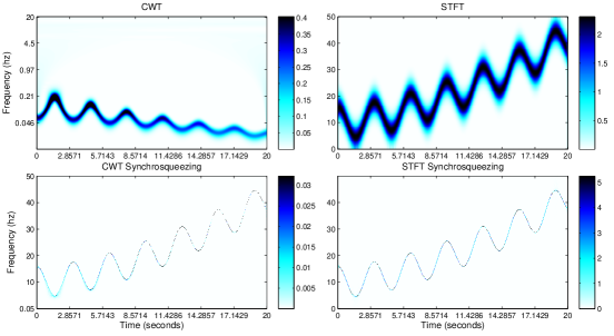
Figure 1: Time-frequency plots of the signal $f(t)=\cos(2\pi(0.1t^{2.6}+3\sin(2t)+10t))$ under different transforms.

3 Theory

Synchrosqueezing has a fairly comprehensive mathematical theory developed for it, providing performance guarantees on selected classes of signals. As of 2014, most of the published theory in [6] and [14] covers the CWT version (4), but analogous results can be shown for the STFT formulation (7) from [15] using similar techniques. We review the results for the CWT case here, which are based on a sparsity model for the signal (1) in the frequency domain.

Definition 1.

For given parameters $\epsilon,d>0$, we define the class $\mathcal{A}_{\epsilon,d}=\{f:f(t)=\sum_{k=1}^{K}A_{k}(t)e^{2\pi i\phi_{k}(t)}\}$, where

$$A_{k}\in L^{\infty}\cap C^{1},\quad\phi_{k}\in C^{2},\quad\phi^{\prime}_{k},\phi^{\prime\prime}_{k}\in L^{\infty},\quad A_{k}(t)>0,\quad\phi_{k}^{\prime}(t)>0$$

$$\forall t\quad\left|A_{k}^{\prime}(t)\right|\leq\epsilon\left|\phi_{k}^{\prime}(t)\right|,\quad\left|\phi_{k}^{\prime\prime}(t)\right|\leq\epsilon\left|\phi_{k}^{\prime}(t)\right|,\quad\mathrm{and}$$

$$\frac{\phi^{\prime}_{k}(t)-\phi^{\prime}_{k-1}(t)}{\phi^{\prime}_{k}(t)+\phi^{\prime}_{k-1}(t)} \geq d.$$ (9)

The key condition here is (9), which says that higher frequency IFs are spaced exponentially further apart than lower frequency IFs. Under this signal model, the following result can be obtained [6].

Theorem 2.

Let $f\in\mathcal{A}_{\epsilon,d}$ for some $\epsilon,d>0$, $h\in C_{0}^{\infty}$ with $\left\|h\right\|_{L^{1}}=1$, and $\psi\in C^{1}$ with $\hat{\psi}$ supported in $[1-\Delta,1+\Delta]$ for some $\Delta<\frac{d}{1+d}$. Let $M$ be sufficiently large and define $\tilde{\epsilon}=\epsilon^{1/3}$ and the “scale band” $Z_{k}=\{(a,b):|a\phi_{k}^{\prime}(t)-1|<\Delta\}$. If $(a,t)\in Z_{k}$ and $|W_{\psi}f(a,t)|>\tilde{\epsilon}$, then $|\omega f(a,t)-\phi_{k}^{\prime}(t)|\leq\tilde{\epsilon}$. Conversely, if $(a,t)\not\in Z_{k}$ for any $k$, then $|W_{\psi}f(a,t)|\leq\tilde{\epsilon}$. Futhermore, for some constant $C_{1}$,

$$\left|\lim_{\delta\rightarrow 0}R_{k,\tilde{\epsilon}}^{\delta,M}f(t)-A_{k}(t)e^{2\pi i\phi_{k}(t)}\right|\leq C_{1}\tilde{\epsilon}.$$

This result says that the energy in the Synchrosqueezing time-frequency plane is concentrated around the IF curves $\{\phi_{k}^{\prime}(t)\}$, and the inverted components $f_{k}$ approximate the actual oscillatory components $\{A_{k}e^{2\pi i\phi_{k}}\}$. Additional results of this type were proved in [14], describing the robustness of the Synchrosqueezing transform under unstructured perturbations (e.g. quantization error) as well as white noise. We slightly paraphrase these theorems for clarity.

Theorem 3.

Let $f$, $\epsilon$, $d$, $h$, $\psi$ and $\Delta$ be given as in Theorem 2. Let $g=f+E$ for some error $E$ with $\left\|E\right\|_{L^{\infty}}$ sufficiently small. There are positive constants $M$, $C_{2}$, $C_{3}$ and $C_{4}$ such that the following holds. Let $a\in[\frac{1}{M},M]$. If $(a,t)\in Z_{k}$ and $|W_{\psi}g(a,t)|>C_{2}\tilde{\epsilon}$, then $|\omega g(a,t)-\phi_{k}^{\prime}(t)|\leq C_{3}\tilde{\epsilon}$. Conversely, if $(a,t)\not\in Z_{k}$ for any $k$, then $|W_{\psi}g(a,t)|\leq C_{2}\tilde{\epsilon}$. Futhermore,

$$\left|\lim_{\delta\rightarrow 0}R_{k,C_{2}\tilde{\epsilon}}^{\delta,M}g(t)-A_{k}(t)e^{2\pi i\phi_{k}(t)}\right|\leq C_{4}\tilde{\epsilon}.$$

   

Theorem 4.

Let $f$, $\epsilon$, $d$, $h$, $\psi$ and $\Delta$ be given as in Theorem 2, with $\psi$ also satisfying $\left|\left\langle\psi,\psi^{\prime}\right\rangle\right|<\left\|\psi\right\|_{L^{2}}\left\|\psi^{\prime}\right\|_{L^{2}}$. Let $g=f+N$, where $N$ is Gaussian white noise with power $\epsilon^{2+p}$ for some $p>0$. There are positive constants $M$, $E_{1}$, $E_{2}$, $C_{2}^{\prime}$, $C_{3}^{\prime}$ and $C_{4}^{\prime}$ such that the following holds. Let $a\in[\frac{1}{M},M]$. If $(a,t)\in Z_{k}$ and $|W_{\psi}g(a,t)|>C_{2}^{\prime}\tilde{\epsilon}$, then with probability $1-e^{-E_{1}\epsilon^{-p}}$, $|\omega g(a,t)-\phi_{k}^{\prime}(t)|\leq C_{3}^{\prime}\tilde{\epsilon}$. Conversely, if $(a,t)\not\in Z_{k}$ for any $k$, then with probability $1-e^{-E_{2}\epsilon^{-p}}$, $|W_{\psi}g(a,t)|\leq C_{2}^{\prime}\tilde{\epsilon}$. Futhermore, with probability $1-e^{-E_{1}\epsilon^{-p}}$,

$$\left|\lim_{\delta\rightarrow 0}R_{k,C_{2}\tilde{\epsilon}}^{\delta,M}g(t)-A_{k}(t)e^{2\pi i\phi_{k}(t)}\right|\leq C_{4}^{\prime}\tilde{\epsilon}.$$

For STFT Synchrosqueezing, a result similar to Theorem 2 was proved in [15], although presented in slightly different terms there. The main distinction with the STFT approach is that the theory is developed for a different function class $\mathcal{B}_{\epsilon,d}$, defined in the same way as $\mathcal{A}_{\epsilon,d}$ in Definition 1 but with (9) replaced by the weaker separation requirement that $\inf_{t}\phi_{k}^{\prime}(t)-\sup_{t}\phi_{k-1}^{\prime}(t)>d$. The linear frequency scale of the modified STFT effectively allows the IF curves $\{\phi_{k}^{\prime}\}$ to be spaced much closer to each other than the logarithmic scale of the CWT. In practical terms, STFT Synchrosqueezing is well suited for decomposing signals with multiple components that have closely packed IFs, especially at higher frequencies, while CWT Synchrosqueezing is more appropriate for studying low frequency, trend-like components in a signal.

We finally mention that the above results have mostly been formulated in a deterministic setting, where the signal of interest $f$ is assumed to lie in the class $\mathcal{A}_{\epsilon,d}$ but without any particular mechanism that generated it. The paper [4] develops extensions of these ideas to a stochastic model of the form $Y(t)=f(t)+T(t)+X(t)$, where $f$ is essentially of the type $\mathcal{A}_{\epsilon,d}$, $T$ is a slowly varying trend and $X$ is an autoregressive moving average (ARMA) process with a time-dependent variance. The authors use CWT Synchrosqueezing to extract the components $f$, $T$ and $X$ from an observed signal $Y$, and prove several results on confidence bounds and other aspects of the decomposition.

4 Applications

Due to its wide applicability, the Synchrosqueezing transform has been used to address problems in many diverse disciplines. The technique was first applied to topics in cardiology, specifically the analysis of electrocardiogram (ECG) signals [15, 17, 18]. The sharp spikes in an ECG signal are called the R peaks (see Figure 2) and encode important information about a patient’s heart rate, respiration and many other physiological properties. The analysis of respiration, or breathing characteristics, is important in many clinical applications such as testing for sleep apnea. However, recording the respiration directly requires hooking up a breathing apparatus (ventilator) to the patient and is often impractical to perform over a long period of time. A patient’s respiration influences the ECG measurement and can be modeled as a low frequency envelope fitting over the R peaks, with the ECG signal’s IF closely following the unobserved respiration signal’s IF. The R peaks are not spaced uniformly but can be used to form an impulse train $\sum_{k}f(t_{k})\delta(\cdot-t_{k})$, where $\{t_{k}\}$ are the locations of the R peaks. Applying the STFT Synchrosqueezing transform to this impulse train provides an IF that accurately reflects short-range frequency variations in the respiration signal (Figure 2), and can be used for diagnosing irregularities in the patient’s breathing.

Synchrosqueezing has also been used for the analysis of long term trends in the global climate. The paper [14] studies sediment cores extracted from the ocean floor, in which the relative concentrations of the oxygen isotopes $\delta^{18}O$ and $\delta^{16}O$ indicate changes in the sea level, ice volume and deep ocean temperature. These are caused by long term fluctuations in the Earth’s eccentricity and other rotational properties over time, known as Milankovitch cycles, which influence the amount of solar radiation received at the top of the atmosphere. The CWT Synchrosqueezing transform is used to analyze the $\delta^{18}O$ levels in several composite stacks of cores over the last 2.5 million years (Figure 3). It is able to distinguish the different Milankovitch cycles more accurately than the regular CWT, commonly used in this field, and identify when certain components faded away or became more prominent. The invertibility of the transform also allows one to extract the oscillatory components corresponding to each of the Milankovitch cycles, and better characterize some sudden changes in the climate between 0.5 and 1 million years ago.

Another application of Synchrosqueezing can be found in economics. The paper [10] studies the stability of the US financial system by considering time-frequency decompositions of equity indices, Treasury yields, foreign exchange rates and several other macroecomonic time series. Each time series is thought of as the output of a dynamical system that produces slowly time-varying frequencies of the form (1), but which are interspersed by abrupt frequency transitions (structural breaks) that indicate the starting or stopping of new underlying dynamics. Among other events, the stock market crash in 1987 is contrasted with the global recession in 2008. It is shown that the former had a minimal impact on the dominant, low frequency components despite being prominent in the original data, while the latter was both preceded and followed by a variety of new dynamics, which left the economy in a permanently altered state (Figure 4). The authors also discuss a measure of instability in a time series called the “density index,” taking the $L^{1}$ norm of the IFs at each point in time as a measure of how spread out or concentrated the frequencies are. A sharp jump in the density index corresponds to a structural break, which is shown to coincide with some of the major financial stress events over the last 25 years and which may provide “early warning” signs of future economic crises.

We briefly mention several other applications of Synchrosqueezing that have appeared in the literature. In [13], it is used to detect and analyze faults in a mechanical gearbox. The Synchrosqueezing plot of the gearbox’s vibration signal reveals extra sideband components surrounding a central IF curve, which indicate the presence of a chipped gear in the transmission. In geophysics, [11] discusses the use of Synchrosqueezing to separate out resonant frequencies in data from micro-seismic experiments, which are used to study deformations in injection wells for oil extraction. Finally, [1] develops an automated trading strategy based on Synchrosqueezing, using the technique to model the relationship between correlated asset pairs such as the stocks of competing firms. The rise in one asset’s price often precedes a fall in the other one, and a strategy based on identifying the prices’ IFs is shown to describe short-range oscillations and outperform some standard approaches used in the industry.

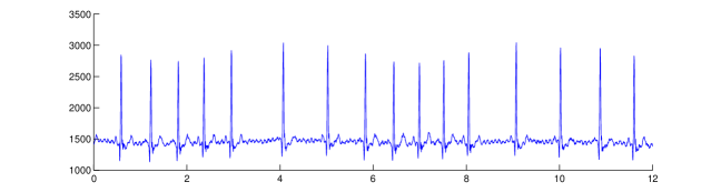
Figure 2: Top: 10 second portion of ECG signal. Bottom: True respiration signal (blue) and the IF computed from the ECG signal’s R peaks (red) using STFT Synchrosqueezing.

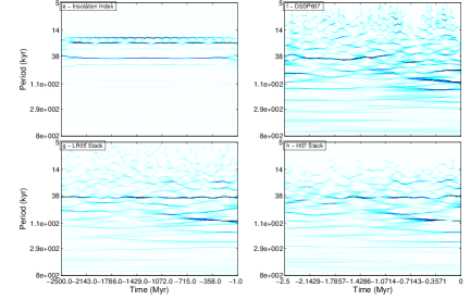
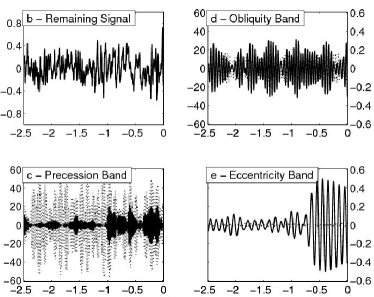
Figure 3: Left: CWT Synchrosqueezing plots of the insolation index, a single core (DSPD07) and stacks of such cores (LR05 and H07). Right: Reconstructed oscillatory components, corresponding to the obliquity, precession and eccentricity cycles.

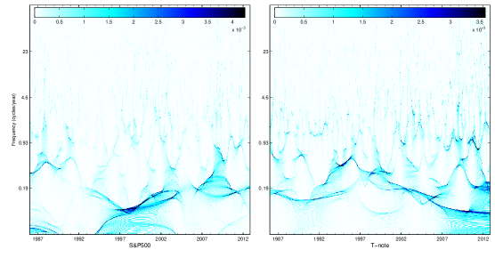
Figure 4: CWT Synchrosqueezing plots of the S&P 500 price and the 10-year US Treasury yield.

References

- [1] A. Ahrabian, C. C. Took, and D. Mandic. Algorithmic Trading Using Phase Synchronization. IEEE Journal of Selected Topics in Signal Processing, 99, 2012.
- [2] F. Auger, P. Flandrin, Y.-T. Lin, S. McLaughlin, S. Meignen, T. Oberlin, and H.-T. Wu. Time-Frequency Reassignment and Synchrosqueezing. IEEE Signal Processing Magazine, pages 32–41, 2013.
- [3] E. Brevdo, G. Thakur, and H.-T. Wu. The Synchrosqueezing Toolbox. 2013. https://web.math.princeton.edu/~ebrevdo/synsq/.
- [4] Y.-C. Chen, M.-Y. Cheng, and H.-T. Wu. Nonparametric and adaptive modeling of dynamic periodicity and trend with heteroscedastic and dependent errors. Journal of the Royal Statistical Society: Series B, 2013.
- [5] I. Daubechies. Ten lectures on wavelets. Society for Industrial and Applied Mathematics, 1992.
- [6] I. Daubechies, J. Lu, and H.-T. Wu. Synchrosqueezed wavelet transforms: An empirical mode decomposition-like tool. Applied and Computational Harmonic Analysis, 30(2):243–261, 2011.
- [7] I. Daubechies and S. Maes. A nonlinear squeezing of the continuous wavelet transform based on auditory nerve models. Wavelets in Medicine and Biology, pages 527–546, 1996.
- [8] P. Flandrin. Time-frequency/time-scale analysis, volume 10 of Wavelet Analysis and its Applications. Academic Press Inc., San Diego, CA, 1999.
- [9] P. Flandrin, F. Auger, and E. Chassande-Mottin. Time-Frequency Reassignment – From Principles to Algorithms. In A. Papandreou-Suppappola, editor, Applications in time-frequency signal processing. CRC, 2003.
- [10] S. K. Guharay, G. S. Thakur, F. J. Goodman, S. L. Rosen, and D. Houser. Analysis of non-stationary dynamics in the financial system. Economics Letters, 121:454–457, 2013.
- [11] R. H. Herrera, J.-B. Tary, and M. van der Baan. Time-frequency representation of microseismic signals using the Synchrosqueezing transform. GeoConvention, 2013.
- [12] C. Li and M. Liang. A generalized synchrosqueezing transform for enhancing signal time-frequency separation. Signal Processing, 92:2264–2274, 2012.
- [13] C. Li and M. Liang. Time-frequency analysis for gearbox fault diagnosis using a generalized synchrosqueezing transform. Mechanical Systems and Signal Processing, 26:205–217, 2012.
- [14] G. Thakur, E. Brevdo, N.-S. Fuckar, and H.-T. Wu. The Synchrosqueezing algorithm for time-varying spectral analysis: robustness properties and new paleoclimate applications. Signal Processing, 93:1079–1094, 2013.
- [15] G. Thakur and H.-T. Wu. Synchrosqueezing-based Recovery of Instantaneous Frequency from Nonuniform Samples. SIAM Journal on Mathematical Analysis, 43(5):2078–2095, 2011.
- [16] H.-T. Wu. Instantaneous frequency and wave shape functions (I). Applied and Computational Harmonic Analysis, 35:181–199, 2013.
- [17] H.-T. Wu, Y.-H. Chan, Y.-T. Lin, and Y.-H. Yeh. Using synchrosqueezing transform to discover breathing dynamics from ECG signals. Applied and Computational Harmonic Analysis, 36(2):354–359, 2014.
- [18] H.-T. Wu, S.-S. Hseu, M.-Y. Bien, Y. R. Kou, and I. Daubechies. Evaluating the physiological dynamics via Synchrosqueezing: Prediction of the Ventilator Weaning. IEEE Transactions on Biomedical Engineering, 2014. to appear.
- [19] H. Yang. Synchrosqueezed Wave Packet Transforms and Diffeomorphism Based Spectral Analysis for 1D General Mode Decompositions. arXiv, 1311.4655, 2013.