Persistence of transition state structure in chemical reactions
driven by fields oscillating in time

Abstract

Chemical reactions subjected to time-varying external forces cannot generally be described through a fixed bottleneck near the transition state barrier or dividing surface. A naive dividing surface attached to the instantaneous, but moving, barrier top also fails to be recrossing-free. We construct a moving dividing surface in phase space over a transition state trajectory. This surface is recrossing-free for both Hamiltonian and dissipative dynamics. This is confirmed even for strongly anharmonic barriers using simulation. The power of transition state theory is thereby applicable to chemical reactions and other activated processes even when the bottlenecks are time-dependent and move across space.

A ubiquitous problem in physics concerns the determination of the mechanism and rate of crossing a bottleneck from initial to final states. In the usual cases, the bottleneck is fixed in time and corresponds to a saddle point (or a ridge of the potential in dimension two or higher) that determines the dynamics. These structures lose their dynamical significance if the potential is time-dependent. However, in those cases in which the barrier moves up and down, perhaps even stochastically, an invariant structure associated with the bottleneck persists Lehmann et al. (2000a, b, 2003); Maier and Stein (2001); Dykman et al. (2004); Dykman and Ryvkine (2005). This is perhaps not surprising because the saddle point of the potential—that is, the barrier top—remains fixed. But what if the position associated with the barrier top moves with time and hence the bottleneck is not fixed? In this Rapid Communication, we show that under some conditions—namely when the motion of the barrier top is periodic—there still exists a fixed structure associated with the bottleneck—the transition state trajectory Bartsch et al. (2005a, b).

This result is of particular interest to chemical physics in which the determination of rates is a central concern, and increasingly rates must be determined in systems that are driven far from equilibrium. Specifically, the response of a chemical constituent to the external forcing by oscillating fields can strongly influence the mechanism and rate in which a reactant is transformed to product. Organic polarization synthesis Lidström et al. (2001) and colloidal and macromolecular structure assembly Elsner et al. (2009); Jäger and Klapp (2011); Prokop et al. (2012); Ma et al. (2013) offer examples of such time-dependent chemical transformations driven under kinetic control.

For field induced molecular dissociation Hiskes (1961), formaldehyde (H₂CO) Moore and Weisshaar (1983); Miller et al. (1990); Butenhoff et al. (1991) can be considered as a prototypical example. The potential energy surface (PES) of formaldehyde contains two dissociation channels (H₂+CO and H+HCO) and isomerization channels to cis-HCOH and trans-HCOH isomers Townsend et al. (2004); Zhang et al. (2004). When H₂CO is subjected to the influence of an external laser field, it is directionally forced. This forcing deforms the PES and influences the reaction rates as well as the placement of the transition state dividing surface. Interest in the construction of a recrossing-free dividing surface (DS) in the bottleneck region of phase space, where reactive trajectories must cross, is not confined to the field of chemical physics Hernandez et al. (2010). For example, bottlenecks play an important role in the dynamics of atoms Jaffé et al. (1999), clusters Komatsuzaki and Berry (1999), microjunctions Eckhardt (1995), asteroids Jaffé et al. (2002), and cosmological spacetime models de Oliveira et al. (2002).

In the absence of a driving field, transition state theory (TST) Truhlar et al. (1983, 1996); Miller (1998); Hernandez et al. (2010) offers a formally exact rate calculation in chemically reactive systems. The methodological hurdle in such calculations is the construction of a hypersurface in phase space that separates reactant and product regions and that is crossed only once by all reactive trajectories. If such a DS cannot be constructed, the TST rate is no longer exact but only an upper bound to the rate. Indeed, variational transition state theory Truhlar and Garrett (1984); Hynes (1985); Pollak (1990); Truhlar and Garrett (2000); Pollak and Talkner (2005); Mullen et al. (2014) has been extremely effective at providing relatively high-accuracy approximations to the rate and the DS. The aim of this article is to resolve the structure of the transition state geometry in situations where the transition state is not fixed because the driving field is oscillatory, advancing previous work by two of us on time-dependent TST Bartsch et al. (2008).

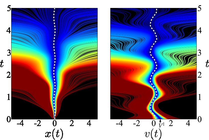
Figure 1: (Color online) Time evolution of $x(t)$ (left) and $v(t)$ (right) for a swarm of 2000 trajectories following the equation of motion (2). The transition state trajectory (TS) is shown in dashed white. The trajectories are colored according to the difference in initial velocity, $\left|V^{\ddagger}-v_{0}\right|$, with respect to the critical velocity $V^{\ddagger}$ as marked. The colors range from dark blue to dark red (or black to gray in grayscale) and are scaled, increasingly, by this difference. Parameters are $\epsilon=2$, $\Omega=5$, $\gamma=3$, $a=1$, and $\varphi=0$.

In an autonomous system with two degrees of freedom, Pechukas and Pollak have shown that the optimal dividing surface is an unstable periodic orbit (PO) Pollak and Pechukas (1978, 1979); Pechukas and Pollak (1979); Pollak et al. (1980). Its projection into configuration space provides a dividing surface that is locally recrossing free. In systems with three or more degrees of freedom, this periodic orbit is generalized to a normally hyperbolic invariant manifold (NHIM) De Leon et al. (1991); Hernandez and Miller (1993); Hernandez (1994); Uzer et al. (2002); Hernandez et al. (2010); Allahem and Bartsch (2012); Li et al. (2006); Waalkens and Wiggins (2004); Çiftçi and Waalkens (2013). Attached to the NHIM are stable and unstable manifolds. These manifolds form phase space separatrices that distinguish between reactive and nonreactive trajectories and also constitute the pathways by which reactive trajectories are funneled from reactant to product through the transition state Uzer et al. (2002); Allahem and Bartsch (2012); Çiftçi and Waalkens (2013). The central result of this article, elaborated below, is that there is a sense in which this structure persists even when the chemical reaction is driven by an external oscillating field as, for example, from an external electric field Kawai et al. (2007); Kawai and Komatsuzaki (2011).

A particle of unit mass propagating from an initial position $x_{0}$ and surmounting a moving one-dimensional energy barrier serves as a paradigm for the present approach. The barrier is moving with a time-dependent, instantaneous position $E(t)$, and is specified by

$$U(x)=-\tfrac{1}{2}\omega_{\text{b}}^{2}(x-E(t))^{2}-\tfrac{1}{4}\epsilon(x-E(t))^{4}.$$ (1)

It leads to the equation of motion

$$\ddot{x}+\gamma\dot{x}=\omega_{\text{b}}^{2}(x-E(t))+\epsilon(x-E(t))^{3},$$ (2)

where $E(t)$ is a driving field, $\gamma$ is a dissipative emission parameter, $\omega_{\text{b}}$ is the barrier frequency, and $\epsilon$ is an anharmonic coefficient. We consider here both the harmonic ($\epsilon=0$) and anharmonic ($\epsilon\neq 0$) cases. In the latter case, the reacting particle’s degree of freedom is non-linearly coupled to the motion of the driving field.

When $\gamma=0$, the system is Hamiltonian and the dynamics are representative of a chemical reaction forced by an external field, such as a laser. The coupling of a molecule’s dipole moment with an external field is known to accelerate the dynamics of a chemical reaction. The collinear H+H₂ exchange reaction is an example of a physical system that can be represented through (2). The asymmetric stretch of the system creates a time-dependent dipole in the region of the one-dimensional TS. The rate of barrier crossing is accelerated when the dipole couples with an external driving field Orel and Miller (1980).

For dissipative ($\gamma>0$) systems, Eq. (2) is a classical approximation for a field-induced reaction undergoing spontaneous emission along a reaction coordinate Argonov and Prants (2008). Herein, we show that when a chemical reaction is forced by a temporally periodic external field, there persists a strictly recrossing-free DS. This recrossing-free criterion is satisfied even for systems that are undergoing a cooling process, i.e., $\gamma>0$.

For every $E(t)$ there exists a specific trajectory that remains close to the energy barrier for all time and never descends into either product or reactant regions. This trajectory has been termed the transition state trajectory (TS) Bartsch et al. (2005a, b, 2006); Revuelta et al. (2012); Bartsch et al. (2012). We will use a time-dependent DS that is located at the instantaneous position of the TS trajectory and show that this DS is recrossing-free, thus confirming that a transition state persists in non-autonomous systems. However, it does not correspond to the location of an energetic saddle point, i.e., an activated complex.

In the harmonic ($\epsilon=0$) case for an arbitrary driving field $E(t)$, Eq. (2) can be solved exactly, with the eigenvalues $\lambda_{\text{s},u}=-\frac{1}{2}\left(\gamma\pm\sqrt{\gamma^{2}+4\omega_{\text{b}}^{2}}\right)$ corresponding to the stable and unstable manifolds. Particular solutions of Eq. (2) can be expressed through the $S$ functionals Bartsch et al. (2005b); Kawai et al. (2007)

$$S_{\tau}[\mu,g;t]=\begin{cases}\displaystyle-\int_{t}^{\infty}g(\tau)\,\exp(\mu(t-\tau))\,d\tau\!\!\!&:\;\operatorname{Re}\mu>0,\\[12.91663pt] \displaystyle+\int_{-\infty}^{t}g(\tau)\,\exp(\mu(t-\tau))\,d\tau\!\!\!&:\;\operatorname{Re}\mu<0,\end{cases}$$ (3)

where $\mu$ is an eigenvalue of (2) and $g(\tau)$ is a time-dependent modulation to the autonomous intramolecular potential. The general solution will contain stable and unstable components, given by (3), and an exponential term which must be omitted to obtain a bounded solution Bartsch et al. (2005b). The TS trajectory is therefore given by Revuelta et al. (2012); Bartsch et al. (2012)

$$x^{\ddagger}(t) =\frac{\omega_{\text{b}}^{2}}{\lambda_{\text{u}}-\lambda_{\text{s}}}\,\left(S[\lambda_{\text{s}},E;t]-S[\lambda_{\text{u}},E;t]\right),$$ (4)

$$v^{\ddagger}(t) =\frac{\omega_{\text{b}}^{2}}{\lambda_{\text{u}}-\lambda_{\text{s}}}\,\left(\lambda_{\text{s}}S[\lambda_{\text{s}},E;t]-\lambda_{\text{u}}S[\lambda_{\text{u}},E;t]\right).$$

Equation (4) gives the TS solution for any $E(t)$, provided only that $\epsilon=0$ and that $E(t)$ is polynomially bounded for $t\to\pm\infty$, such that the $S$ functionals exist.

We now restrict the discussion to sinusoidally oscillating fields of the form

$$E(t)=a\sin(\Omega t+\varphi),$$ (5)

although the methods presented herein apply equally to arbitrary periodic oscillations. With this restriction, the TS trajectory, given by Eq. (4), is an unstable PO whose period $2\pi/\Omega$ is the period of the external driving. In systems with anharmonic barriers, we will therefore choose an unstable PO close to the barrier top as the TS trajectory. The TS trajectory acts like a moving saddle point: Like the equilibrium point on the autonomous barrier, it remains in the transition region for all time. Trajectories that begin on the stable manifold approach it, asymptotically, as $t\to\infty$. All other trajectories move away in the infinite future.

Fig. 1 shows the time evolution of $x(t)$ and $v(t)$ for a set of trajectories starting at some point $x_{0}$ to the left of the barrier. Specifically, the potential (1) describes an inverted (an)harmonic oscillator. Initial velocities are sampled from a Boltzmann distribution $q(v)$. For all numerical simulations in this paper, we have chosen units such that the particle mass, the barrier frequency $\omega_{\text{b}}$ and the thermal energy $k_{\text{B}}T$ of the initial Boltzmann distribution are unity; all other parameters are dimensionless. Most trajectories in Fig. 1 quickly move away from the DS in accordance with the unstable nature of the PO. As a consequence of this instability, the Poincaré return map that records the phase space position of a trajectory after each period of the driving contains very little information Though not shown, it has a single fixed point arising from the TS trajectory and only a few returns for the escaping trajectories.

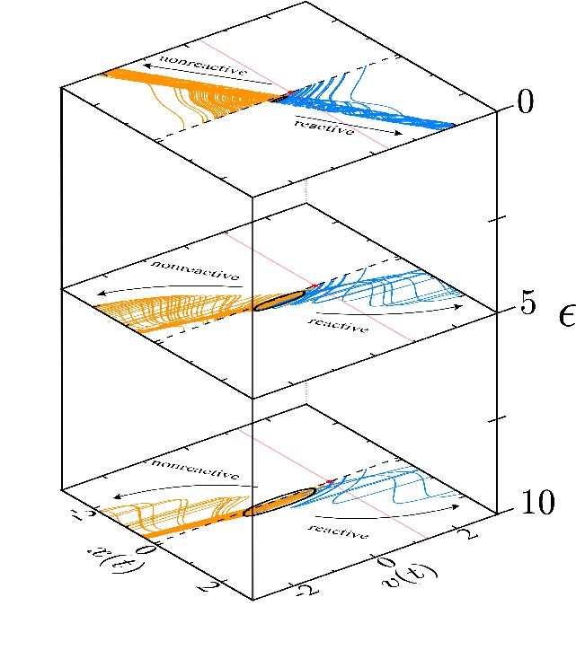
Figure 2: (Color online) A swarm of 100 trajectories starting at $x_{0}$ (dashed black line) propagated by Eq. (2) at $\epsilon=0$, 5 and 10. Reactive and nonreactive trajectories are identified by labeled arrows. The TS trajectory is a periodic orbit in solid black. The critical velocity $V^{\ddagger}$ lies at the vertex of $x_{0}$ and the grey (red) line. Parameters are $\Omega=5$, $\gamma=1$, $a=1$, and $\varphi=0$.

Some trajectories, however, remain close to the TS trajectory for long times. Indeed, given an initial position, there exists a unique trajectory that approaches the TS trajectory asymptotically with increasing time. It can be specified by its initial velocity, which we call the critical velocity $V^{\ddagger}$. This particular trajectory lies on the stable manifold of the TS trajectory (which by definition contains all those trajectories that asymptotically approach the TS trajectory as $t\to\infty$). Trajectories close to the stable manifold are captured in the vicinity of the TS trajectory for a long time before they finally descend into either the reactant or the product wells. The stable manifold itself contains trajectories that will never descend. It therefore separates reactive from nonreactive trajectories in phase space: Trajectories whose initial velocity is larger than $V^{\ddagger}$ are reactive, those with initial velocities below $V^{\ddagger}$ are not.

In our numerical computation, we choose initial conditions on the line $x=x_{0}=-0.1$. The stable manifold intersects this line at the point $(x_{0},V^{\ddagger})$. In the present case, the critical velocity is $V^{\ddagger}\approx 0.819$ as highlighted in Fig. 1. Note that it is not the velocity of the instantaneous barrier top, which is $a\Omega=5$ at $t=0$.

The TS trajectory also defines a moving DS, $x=x^{\ddagger}(t)$, that can be used to track the reactant and product populations in the generic reaction $\text{R}\rightarrow\text{P}$. The normalized reactant population $P_{\text{R}}(t)$ is the fraction of trajectories that are on the reactant side of the TS trajectory, relative to the moving DS, at time $t$. In a two-state model, the normalized product population is $P_{\text{P}}(t)=1-P_{\text{R}}(t)$. A monotonic behavior in these populations indicates that the chosen DS is recrossing-free.

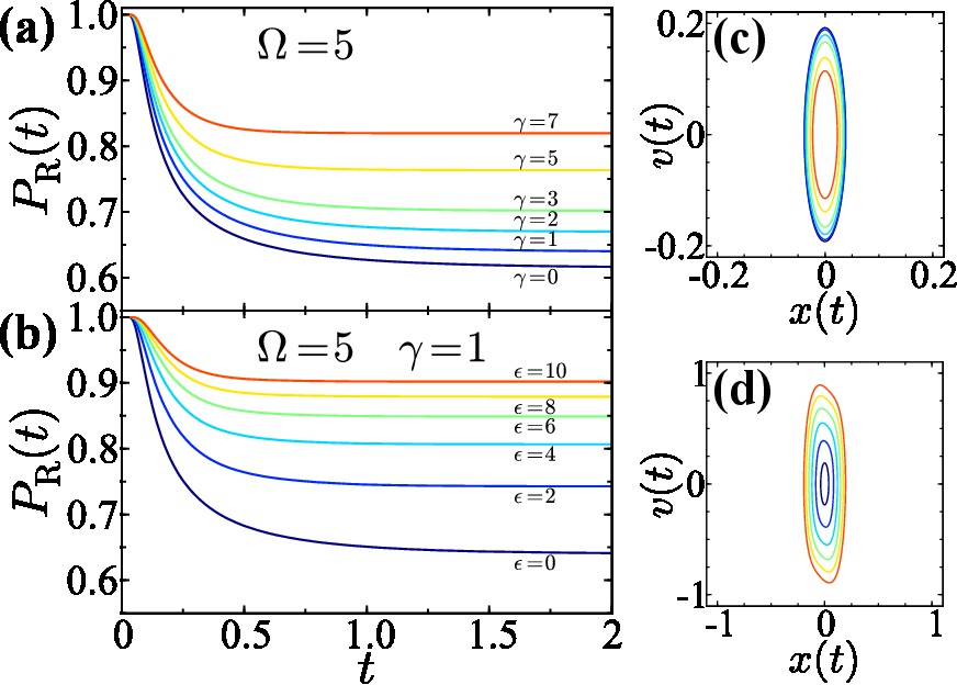
Figure 3: (Color online) Reactant populations as a function of time for the harmonic (a) and anharmonic (b) barrier. The corresponding TS trajectories are shown in panels (c) and (d), respectively. In all cases, $a=1$, and $\varphi=0$.

A reactive trajectory will cross the moving DS $x=x^{\ddagger}(t)$ at a time $t^{\ddagger}(v)$ that depends on the initial velocity. At any time $t>0$, the product region $(x(t)-x^{\ddagger}(t))>0$, to the right of the moving surface, will contain all those trajectories that cross the surface at a time $t^{\ddagger}<t$. These are the trajectories that have an initial velocity of at least $v_{\text{min}}$, where $t^{\ddagger}(v_{\text{min}}-v^{\ddagger}(0))=t$. From this condition and the expression of $t^{\ddagger}$ derived in Ref. Bartsch et al., 2006, for a harmonic barrier, $v_{\text{min}}$ can be obtained exactly and is given by

$$v_{\text{min}}(t)=v^{\ddagger}(0)+\frac{\lambda_{\text{u}}e^{-\lambda_{\text{u}}t}-\lambda_{\text{s}}e^{-\lambda_{\text{s}}t}}{e^{-\lambda_{\text{u}}t}-e^{-\lambda_{\text{s}}t}}\,(x_{0}-x^{\ddagger}(0)).$$ (6)

The population of the reactant region at time $t$ is therefore

$$P_{\text{R}}(t)=\int_{-\infty}^{v_{\text{min}}(t)}q(v)\,dv.$$ (7)

The critical velocity $V^{\ddagger}$ is the long-time limit of $v_{\text{min}}(t)$. Because $V^{\ddagger}$ is a time-invariant identifier of reactive trajectories, the reactant population in the long-time limit is

$$P_{\text{R}}(\infty)=\int_{-\infty}^{V^{\ddagger}}q(v)\,dv,$$ (8)

which is the fraction of trajectories that never surmount the barrier.

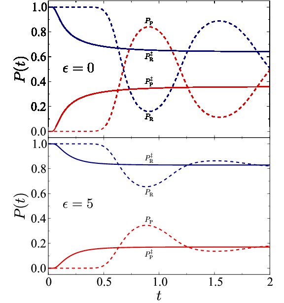
Figure 4: (Color online) Time dependence of the reactant $P_{\text{R}}$ and product $P_{\text{P}}$ populations for harmonic and anharmonic barriers obtained relative to the instantaneous barrier top (dashed lines) and the TS trajectory (solid lines). All other parameters as in Fig. 2.

For an anharmonic barrier, Eqs. (7), and (8) are valid, although $v_{\text{min}}(t)$ is, in general, not known exactly. Fig. 2 illustrates trajectories for various strengths of the anharmonicity. The critical velocity, shown as a red circle, marks the boundary between reactive and nonreactive trajectories. The reactive trajectories trace the forward branch of the unstable manifold while the nonreactive trajectories trace the backward branch. The location of a trajectory’s initial velocity with respect to $V^{\ddagger}$ decides which branch the trajectory follows as it moves toward its final state. It can also be seen in Fig. 2 that $V^{\ddagger}$ increases with increasing $\epsilon$, and thus increasing the anharmonicity decreases the amount of product formed. This increase in $V^{\ddagger}$ is due to the curvature in the stable and unstable manifolds that is induced by anharmonicity.

To test that the DS is recrossing-free, we simulated ensembles of $10^{6}$ trajectories with an initial position $x_{0}=-0.1$ to the left of the instantaneous barrier top and initial velocities sampled from a Boltzmann distribution. For every time $t$ we compute the normalized reactant population $P_{\text{R}}(t)$ and the normalized product population $P_{\text{P}}(t)$. The time evolution of $P_{\text{R}}(t)$ for varying parameters values is shown in Fig. 3. The harmonic case is shown in Fig. 3(a) with the corresponding TS trajectories in Fig. 3(c). The anharmonic case is shown in Fig. 3(b) with corresponding TS trajectories shown in Fig. 3(d). In all cases, the DS is free of recrossings, as is evident from the observation that the reactant populations decrease monotonically.

This is in stark contrast to the reactant and product populations that are obtained from a DS attached to the instantaneous barrier top. That surface can be recrossed many times. As a consequence, reactant and product populations determined from this surface are not monotonic, but show pronounced oscillations as a function of time, as shown in Fig. 4. Using the instantaneous barrier top as a DS, in accordance with the canonical view of the transition state, an observer would alternatingly overestimate and underestimate the reactive portion of the ensemble of initial conditions. Populations obtained from the recrossing-free DS not only converge faster to their long-time asymptotic values, they also approach these values monotonically and thereby provide rigorous upper or lower bounds for the limiting values.

In summary, we have studied the dynamics of a reactant particle surmounting an oscillating energy barrier. A dividing surface attached to a bounded transition state trajectory has been constructed that is rigorously free from recrossing, even when the dynamics is strongly anharmonic, strongly dissipative, or strongly driven. In addition, whether a trajectory is reactive or not is determined by its location relative to the stable manifold of the transition state trajectory. The knowledge of the stable manifold therefore allows prediction of the fate (reactive or nonreactive) of any trajectory, without having to carry out a simulation. The validity of these results has been confirmed by a numerical simulation of ensembles of trajectories. The construction of this dividing surface allows for a formally exact TST rate calculations in periodically driven chemical reactions which we are pursuing in current work.

This work has been partially supported by the National Science Foundation (NSF) through Grant No. NSF- CHE-1112067. Travel between partners was partially supported through the People Programme (Marie Curie Actions) of the European Union’s Seventh Framework Programme FP7/2007-2013/ under REA Grant Agreement No. 294974.

References

- Lehmann et al. (2000a) J. Lehmann, P. Reimann, and P. Hänggi, Phys. Rev. Lett. 84, 1639 (2000a), doi:10.1103/PhysRevLett.84.1639 .
- Lehmann et al. (2000b) J. Lehmann, P. Reimann, and P. Hänggi, Phys. Rev. E 62, 6282 (2000b), doi:10.1103/PhysRevE.62.6282 .
- Lehmann et al. (2003) J. Lehmann, P. Reimann, and P. Hänggi, Phys. Status Solidi B 237, 53 (2003), doi:10.1002/pssb.200301774 .
- Maier and Stein (2001) R. S. Maier and D. L. Stein, Phys. Rev. Lett. 86, 3942 (2001), doi:10.1103/PhysRevLett.86.3942 .
- Dykman et al. (2004) M. I. Dykman, B. Golding, and D. Ryvkine, Phys. Rev. Lett. 92, 080602 (2004), doi:10.1103/PhysRevLett.92.080602 .
- Dykman and Ryvkine (2005) M. I. Dykman and D. Ryvkine, Phys. Rev. Lett. 94, 070602 (2005), doi:10.1103/PhysRevLett.94.070602 .
- Bartsch et al. (2005a) T. Bartsch, R. Hernandez, and T. Uzer, Phys. Rev. Lett. 95, 058301 (2005a), doi:10.1103/PhysRevLett.95.058301 .
- Bartsch et al. (2005b) T. Bartsch, T. Uzer, and R. Hernandez, J. Chem. Phys. 123, 204102 (2005b), doi:10.1063/1.2109827 .
- Lidström et al. (2001) P. Lidström, J. Tierney, B. Wathey, and J. Westman, Tetrahedron 57, 9225 (2001), doi:10.1016/S0040-4020(01)00906-1 .
- Elsner et al. (2009) N. Elsner, C. P. Royall, B. Vincent, and D. R. E. Snoswell, J. Chem. Phys. 130, 154901 (2009), doi:10.1063/1.3115641 .
- Jäger and Klapp (2011) S. Jäger and S. H. L. Klapp, Soft Matter 7, 6606 (2011), doi:10.1039/c1sm05343d .
- Prokop et al. (2012) A. Prokop, J. Vacek, and J. Michl, ACS Nano 6, 1901 (2012), doi:10.1021/nn300003x .
- Ma et al. (2013) F. Ma, D. T. Wu, and N. Wu, J. Am. Chem. Soc. 135, 7839 (2013), doi:10.1021/ja403172p .
- Hiskes (1961) J. R. Hiskes, Phys. Rev. 122, 1207 (1961), doi:10.1103/PhysRev.122.1207 .
- Moore and Weisshaar (1983) C. B. Moore and J. C. Weisshaar, Annu. Rev. Phys. Chem. 34, 525 (1983), doi:10.1146/annurev.pc.34.100183.002521 .
- Miller et al. (1990) W. H. Miller, R. Hernandez, C. B. Moore, and W. F. Polik, J. Chem. Phys. 93, 5657 (1990), doi:10.1063/1.459636 .
- Butenhoff et al. (1991) T. J. Butenhoff, K. L. Carleton, R. D. van Zee, and C. B. Moore, J. Chem. Phys. 94, 1947 (1991), doi:10.1063/1.459916 .
- Townsend et al. (2004) D. Townsend, S. A. Lahankar, S. K. Lee, S. D. Chambreau, A. G. Suits, X. Zhang, J. Rheinecker, L. B. Harding, and J. M. Bowman, Science 306, 1158 (2004), doi:10.1126/science.1104386 .
- Zhang et al. (2004) X. Zhang, S. Zou, L. B. Harding, and J. M. Bowman, J. Phys. Chem. A 108, 8980 (2004), doi:10.1021/jp048339l .
- Hernandez et al. (2010) R. Hernandez, T. Bartsch, and T. Uzer, Chem. Phys. 370, 270 (2010), doi:10.1016/j.chemphys.2010.01.016 .
- Jaffé et al. (1999) C. Jaffé, D. Farrelly, and T. Uzer, Phys. Rev. A 60, 3833 (1999), doi:10.1103/PhysRevA.60.3833 .
- Komatsuzaki and Berry (1999) T. Komatsuzaki and R. S. Berry, J. Chem. Phys. 110, 9160 (1999), doi:10.1063/1.478838 .
- Eckhardt (1995) B. Eckhardt, J. Phys. A 28, 3469 (1995), doi:10.1088/0305-4470/28/12/019 .
- Jaffé et al. (2002) C. Jaffé, S. D. Ross, M. W. Lo, J. Marsden, D. Farrelly, and T. Uzer, Phys. Rev. Lett. 89, 011101 (2002), doi:10.1103/PhysRevLett.89.011101 .
- de Oliveira et al. (2002) H. P. de Oliveira, A. M. Ozorio de Almeida, I. Damiõ Soares, and E. V. Tonini, Phys. Rev. D 65, 083511/1 (2002), doi:10.1103/PhysRevD.65.083511 .
- Truhlar et al. (1983) D. G. Truhlar, W. L. Hase, and J. T. Hynes, J. Phys. Chem. 87, 2664 (1983), doi:10.1021/j100238a003 .
- Truhlar et al. (1996) D. G. Truhlar, B. C. Garrett, and S. J. Klippenstein, J. Phys. Chem. 100, 12771 (1996), doi:10.1039/A805196H .
- Miller (1998) W. H. Miller, Faraday Discuss. Chem. Soc. 110, 1 (1998), doi:10.1039/A805196H .
- Truhlar and Garrett (1984) D. G. Truhlar and B. C. Garrett, Annu. Rev. Phys. Chem. 35, 159 (1984), doi:10.1146/annurev.pc.35.100184.001111 .
- Hynes (1985) J. T. Hynes, Annu. Rev. Phys. Chem. 36, 573 (1985), doi:10.1146/annurev.pc.36.100185.003041 .
- Pollak (1990) E. Pollak, J. Chem. Phys. 93, 1116 (1990).
- Truhlar and Garrett (2000) D. G. Truhlar and B. C. Garrett, J. Phys. Chem. B 104, 1069 (2000), doi:10.1021/jp992430l .
- Pollak and Talkner (2005) E. Pollak and P. Talkner, Chaos 15, 026116 (2005).
- Mullen et al. (2014) R. G. Mullen, J.-E. Shea, and B. Peters, J. Chem. Phys. 140, 041104 (2014), doi:10.1063/1.4862504 .
- Bartsch et al. (2008) T. Bartsch, J. M. Moix, R. Hernandez, S. Kawai, and T. Uzer, Adv. Chem. Phys. 140, 191 (2008).
- Pollak and Pechukas (1978) E. Pollak and P. Pechukas, J. Chem. Phys. 69, 1218 (1978), doi:10.1063/1.436658 .
- Pollak and Pechukas (1979) E. Pollak and P. Pechukas, J. Chem. Phys. 70, 325 (1979), doi:10.1063/1.437194 .
- Pechukas and Pollak (1979) P. Pechukas and E. Pollak, J. Chem. Phys. 71, 2062 (1979), doi:10.1063/1.438575 .
- Pollak et al. (1980) E. Pollak, M. S. Child, and P. Pechukas, J. Chem. Phys. 72, 1669 (1980), doi:10.1063/1.439276 .
- De Leon et al. (1991) N. De Leon, M. A. Mehta, and R. Q. Topper, J. Chem. Phys. 94, 8310 (1991).
- Hernandez and Miller (1993) R. Hernandez and W. H. Miller, Chem. Phys. Lett. 214, 129 (1993), doi:10.1016/0009-2614(93)90071-8 .
- Hernandez (1994) R. Hernandez, J. Chem. Phys. 101, 9534 (1994), doi:10.1063/1.467985 .
- Uzer et al. (2002) T. Uzer, C. Jaffé, J. Palacián, P. Yanguas, and S. Wiggins, Nonlinearity 15, 957 (2002), doi:10.1088/0951-7715/15/4/301 .
- Allahem and Bartsch (2012) A. Allahem and T. Bartsch, J. Chem. Phys. 137, 214310 (2012), doi:10.1063/1.4769197 .
- Li et al. (2006) C.-B. Li, A. Shoujiguchi, M. Toda, and T. Komatsuzaki, Phys. Rev. Lett. 97, 028302 (2006), doi:10.1103/PhysRevLett.97.028302 .
- Waalkens and Wiggins (2004) H. Waalkens and S. Wiggins, J. Phys. A 37, L435 (2004), doi:10.1088/0305-4470/37/35/L02 .
- Çiftçi and Waalkens (2013) U. Çiftçi and H. Waalkens, Phys. Rev. Lett. 110, 233201 (2013), 10.1103/PhysRevLett.110.233201 .
- Kawai et al. (2007) S. Kawai, A. D. Bandrauk, C. Jaffé, T. Bartsch, J. Palacián, and T. Uzer, J. Chem. Phys. 126, 164306 (2007), doi:10.1063/1.2720841 .
- Kawai and Komatsuzaki (2011) S. Kawai and T. Komatsuzaki, J. Chem. Phys. 134, 024317 (2011), doi:10.1063/1.3528937 .
- Orel and Miller (1980) A. E. Orel and W. H. Miller, J. Chem. Phys. 72, 5139 (1980), doi:10.1063/1.439747 .
- Argonov and Prants (2008) V. Y. Argonov and S. V. Prants, Phys. Rev. A 78, 043413 (2008), doi:10.1103/PhysRevA.78.043413 .
- Bartsch et al. (2006) T. Bartsch, T. Uzer, J. M. Moix, and R. Hernandez, J. Chem. Phys. 124, 244310(01) (2006), doi:10.1063/1.2206587 .
- Revuelta et al. (2012) F. Revuelta, T. Bartsch, R. M. Benito, and F. Borondo, J. Chem. Phys. 136, 091102 (2012), doi:10.1063/1.3692182 .
- Bartsch et al. (2012) T. Bartsch, F. Revuelta, R. M. Benito, and F. Borondo, J. Chem. Phys. 136, 224510 (2012), doi:10.1063/1.4726125 .