Rayleigh scattering in coupled microcavities: Theory

Abstract

In this paper we theoretically study how structural disorder in coupled semiconductor heterostructures influences single-particle scattering events that would otherwise be forbidden by symmetry. We extend the model of V. Savona Savona (2007) to describe Rayleigh scattering in coupled planar microcavity structures, and answer the question, whether effective filter theories can be ruled out. They can.

I Introduction

Resonant Rayleigh scattering (RRS) caused by the structural disorder of semiconductor heterostructures is a well-known phenomenon in semiconductor optics. It is usually regarded as an unwanted feature, however, it has recently been realised that it can be exploited to study fundamental effects, e.g., to probe for polariton superfluidity Carusotto and Ciuti (2004), or measure the properties of a polariton condensate Christmann et al. (2012). Recently, there have also been attempts at influencing RRS by inducing strain in the heterostructures Zajac et al. (2012), or by superposing a periodic potential on the random disorder Abbarchi et al. (2012).

In the early stages of RRS experiments, when the phenomenon was first observed in polaritonic systems, it was not clear, what exactly causes Rayleigh scattering: since polaritons are a coherent superposition of quantum well excitons and cavity photons, in principle, either of the constituents could be affected by structural disorder. However, given that RRS did not show a strong temperature dependence, and that it could be observed even in cavities without quantum well excitons (so-call cold cavities), it was soon established that photonic imperfections of the structures are responsible Houdré et al. (2000); Houdre2001; Gurioli et al. (2001, 2002, 2003); Langbein (2004, 2010); Zajac and Langbein (2012).

Due to the resonant nature of the scattering, in single microcavities, the final states will be distributed on a circle, that can easily be distinguished in the far-field emission pattern. It is important to realize that in such a case, scattering happens on a single branch, given that the lower and upper polaritons are energetically separated. However, when one couples two such cavities through partially reflecting mirrors, the resulting eigenmodes of the system overlap energetically. It is only natural to ask, whether RRS still happens only on the branch that is pumped (intra-branch scattering), and if this is not the case, what determines the conditions for scattering to the unpumped branch (inter-branch scattering). What makes the problem even more interesting, is the fact that in a perfect structure (i.e., one without disorder), inter-branch scattering would be forbidden by the reflection symmetry (parity) of the system, and one could then ask, to what extent disorder breaks this symmetry. The answers to these questions have also some practical consequences: some of the parametric scattering schemes that attempt to generate quantum correlated light are degenerate, and it is of paramount importance to find out, whether parametric luminescence has to compete with RRS, which would reduce the quantum nature of the generated light.

However, even after it was established that only photons undergo Rayleigh scattering, there could still be various ways in which scattering could happen. The simplest explanation is given by the so-called filter theory, which states that the intra-cavity light field is scattered by the disorder inside the cavity producing a spherical wave, and only those components of the scattered field can be detected outside that are resonant with the cavity, for the other components will be attenuated. In this regard, symmetry plays no role in the scattering process, and the situation is identical to that of a Fabry-Pérot resonator with a diffusive plate between the mirrors Freixanet et al. (1999). In particular, since the cavity filters the modes of the spherical wave, it is assumed in this model that the cavity mirrors are perfect.

A cavity consists of two mirrors, and the enclosed space. The filter theory assumes that scattering happens in the enclosed space. But RRS could also be caused by the imperfections of the mirrors. This is the starting point of the theory of V. Savona Savona (2007); Sarchi et al. (2009), in which he proves rigorously that because of the large effective mass of the exciton (about 5 orders of magnitude larger than that of the photons), the effect of excitonic disorder is negligible in RRS. While his theory accounts for all the observed phenomena, it still cannot unambiguously rule out the filter theory. In this contribution, we extend his theory to multiple cavities, and we analyse the case of double cavities in detail. For such structures, the filter theory would predict that the scattered spherical wave would be filtered by two resonances, resulting in the far field in two concentric rings with approximately equal powers. Savona’s theory, on the other hand, predicts that the far field emission will contain the same two concentric rings as in the filter theory, but their relative intensities will depend on the correlations of the photonic disorder. It can thus be expected that a measurement on the relative intensities of the two rings would differentiate between the two models.

In the first half of the paper, in Section II., we outline the underlying principles of Savona’s theory of Rayleigh scattering in a single microcavity. In Section III., we introduce simplifications that do not change the main conclusions, and extend the model to the case of coupled cavities. We solve the simplified equations numerically, and show that in coupled cavities, longitudinal correlations of the the disorder potential are the relevant parameter of RRS. While this model is conceptually simple, it can only be solved numerically. In the second part of the paper, starting with Section IV., we apply perturbation theory, and develop a simple analytical model that can reproduce most of the results of the numerical simulations. In the appendix, we show how this model can be extended to triple cavities, a rather popular experimental realization of coupled cavities. We conclude with a short conclusion and outlook.

II Rayleigh scattering in a single microcavity

First we re-capitulate Savona’s theory of for the case of a single cavity. The extension of the model to an arbitrary number of cavities is straightforward. The theory is based on the assumption that the electric field inside the cavity can be written as

$$E(\mathbf{r},z)=E(\mathbf{r})\exp(ik_{z}(\mathbf{r})z)\,,$$

where $k_{z}(\mathbf{r})$ is the position-dependent photon momentum along the $z$ direction, and $\mathbf{r}$ lies in the plane of the cavities. Above, only a single mode is considered, therefore, the polarization degree of freedom plays no role. By introducing the macroscopic exciton polarization field $P(\mathbf{r})$, the Helmholtz equation

$$\nabla_{\mathbf{r}}^{2}E(\mathbf{r})+\left(\frac{\omega_{p}}{c^{2}}\epsilon_{0}-k_{z}^{2}(\mathbf{r})\right)E(\mathbf{r})+4\pi\frac{\omega^{2}}{c^{2}}P(\mathbf{r})=0$$

can then be expanded around the mean cavity length, $\lambda_{0}$, resulting in an effective Schrödinger equation for the photon mode

$$i\hbar\frac{\partial E(\mathbf{r},z,t)}{\partial t} = -\frac{\hbar^{2}}{2m_{p}}\nabla_{\mathbf{r}}^{2}E(\mathbf{r},t)+V_{p}(\mathbf{r})E(\mathbf{r},t)$$ (1)

$$\qquad-2\pi\frac{\hbar\omega_{p}}{\epsilon_{0}}P(\mathbf{r},t)$$

where the effective mass of the photon is given by the expressions

$$m_{p}=\frac{\hbar\omega_{p}}{2c^{2}}\qquad\mathrm{and}\qquad\omega_{p}=\frac{2\pi c}{n\left(\lambda_{0}+L_{\mathrm{DBR}}\right)}\,,$$

where $L_{\mathrm{DBR}}$ is the penetration length of the electric field into the distributed Bragg reflector (DBR), and $n$ is the refractive index of the cavity. The disorder potential, $V_{p}(\mathbf{r})$, stems from the local variations of the cavity length, $\delta L(\mathbf{r})$, as

$$V_{p}(\mathbf{r})=\frac{\hbar c}{\sqrt{\epsilon_{0}}}\delta k_{z}(\mathbf{r})=-\hbar\omega_{p}\frac{\delta L(\mathbf{r})}{\lambda_{0}+L_{\mathrm{DBR}}}\,.$$

Eq. (1) can be completed by noticing that the polarization, $P(\mathbf{r})$, depends linearly on the center-of-mass wave function $\Psi(\mathbf{r},t)$ of the exciton Savona et al. (2000), whence one arrives at the coupled equations

$$i\hbar\frac{\partial E(\mathbf{r},t)}{\partial t} = \hbar\omega_{p}(\mathbf{r})E(\mathbf{r},t)-\frac{\hbar^{2}}{2m_{p}}\nabla_{\mathbf{r}}^{2}E(\mathbf{r},t)+V_{p}(\mathbf{r})E(\mathbf{r},t)+\frac{\hbar\Omega_{R}}{2}\Psi(\mathbf{r},t)+f(\mathbf{r},t)$$ (2)

$$i\hbar\frac{\partial\Psi(\mathbf{r},t)}{\partial t} = \hbar\omega_{x}(\mathbf{r})E(\mathbf{r},t)-\frac{\hbar^{2}}{2m_{x}}\nabla_{\mathbf{r}}^{2}\Psi(\mathbf{r},t)+V_{x}(\mathbf{r})\Psi(\mathbf{r},t)+\frac{\hbar\Omega_{R}}{2}E(\mathbf{r},t)\,,$$ (3)

Eqs. (2-3) constitute the equation of motion of the coupled photon-exciton system. All quantities with the subscript $x$ refer to the exciton component, while the subscript $p$ stands for the cavity photon. $f(\mathbf{r},t)$ is a source term that generates intracavity photons (and through the coupling, excitons), while $\omega_{p}(\mathbf{r})$, and $\omega_{x}(\mathbf{r})$ contain the photonic and excitonic disorder, and the finite lifetime. Consequently, the frequencies can have imaginary parts. Without disorder, these equations can be diagonalized, resulting in two new eigenmodes, the so-called upper and lower polaritons, whose splitting in energy is usually called the Rabi splitting, $\hbar\Omega_{R}$.

When the disorder is not zero, due to the large mis-match of the exciton and photon effective masses, the numerical solution of these two equations is not trivial, and requires huge resources. However, a key observation that can be drawn from Savona’s calculations is that Rayleigh scattering is dominated by the photonic disorder, and the sole role of the quantum well exciton is to modify the dispersion relations of the polariton states. This statement is also confirmed by the experimental results of Maragkou et al., where Rayleigh scattering was observed even in a cold cavity Maragkou et al. (2011). For this reason, we will drop the equation for the exciton wavefunction. In cases, where accurate modeling of the polariton states is required, in order to reduce the computation costs, one can introduce higher-order derivatives in Eq. (2), so as to better approximate the non-parabolicity of the dispersion. However, since this would not qualitatively change our results, we will not pursue this route here.

III Coupled cavities

III.1 Model equations

Having discussed the case of a single cavity, we now turn to the derivation of the equation of motion in coupled microcavities.

The system under consideration is depicted in Fig. 1: two cavities are coupled through a partially transparent DBR. Quantum wells are located in the center of the cavities. The disorder of the mirrors is symbolized by their rugged surface.

Out of the two longitudinally localized photonic modes (red solid lines in Fig. 1), the coupling produces four polariton eigenstates that are split. Just as in the single cavity case, the lower polaritons are still energetically separated from the upper polaritons, but both the upper, and the lower polaritons overlap spectrally. This raises the possibility of scattering processes in which no energy is exchanged, but which take a polariton from one branch to another (inter-branch scattering), as shown on the right hand side of Fig. 1. While in a perfect cavity such processes would be forbidden by the conservation of parity, for a disordered system parity is not a good quantum number anymore. In the rest of the paper, we will study how inter-branch scattering depends on the properties of the disorder that breaks the parity symmetry.

As mentioned above, in order to simplify the description, we drop the excitonic component. We note, nevertheless, that in coupled cavities, one can still retain the excitonic wavefunction, but the coupling will be mediated by the photonic part only: excitons are confined to their respective quantum wells, and in realistic experimental situations, exciton tunneling between two quantum wells can safely be ignored Einkemmer et al. (2013).

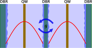
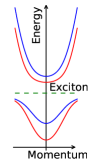
Figure 1: Left: The system under consideration. The disorder potential acting on the photonic modes is the rugged mirror surface. The two uncoupled modes are the solid red lines, while the coupling of the cavities, $g$, is symbolized by the blue arrows. Right: schematic polariton dispersions in a coupled cavity at zero detuning. Also shown is the exciton line in dashed green.

In what follows, we will denote the transverse wavefunction of the photon fields in the two cavities by $E_{a,b}(\mathbf{r},t)$, the corresponding energies by $\omega_{a,b}(\mathbf{r})$, the photon effective masses by $m_{a,b}$, and the source terms by $f_{a,b}$.

Moreover, we denote the coupling of the two cavities by $g_{0}$. In general, the transmission of the DBRs depends on the wavevector, and by applying the standard transfer matrix approach, it can be shown that this dependence results in a correction quadratic in the length of the wavevector. In the momentum space equations, this correction can be accounted for by adding the Laplace operator to the coupling constant as $\epsilon\nabla^{2}$. However, in subsequent calculations, we drop this term, for it only modifies the dispersion relations, but has no other bearing on our results.

The energies $\omega_{a,b}(\mathbf{r})$ depend, on the one hand, on the length of the cavities (as do the effective masses $m_{a,b}$), and on the other hand, on the disorder potential. It is because of this spatially inhomogeneous disorder potential that the usual Bogolyubov transformation cannot be carried out, and that we cannot decompose the eigenmodes of the coupled system as a symmetric and an anti-symmetric linear combination of the original states.

With these considerations, the two equations governing the time-evolution of the two modes in question are

$$\frac{\partial E_{a}(\mathbf{r},t)}{\partial t} = i\omega_{a}(\mathbf{r})E_{a}(\mathbf{r},t)+\frac{i}{m_{a}}\nabla^{2}E_{a}(\mathbf{r},t)+i(g_{0}-\epsilon\nabla^{2})E_{b}(\mathbf{r},t)+f_{a}(\mathbf{r},\omega_{0},t)$$ (4)

$$\frac{\partial E_{b}(\mathbf{r},t)}{\partial t} = i\omega_{b}(\mathbf{r})E_{b}(\mathbf{r},t)+\frac{i}{m_{b}}\nabla^{2}E_{b}(\mathbf{r},t)+i(g_{0}-\epsilon\nabla^{2})E_{a}(\mathbf{r},t)+f_{b}(\mathbf{r},\omega_{0},t)\,.$$ (5)

In the following, we will assume that the two cavities have the same length, and a disorder potential with the same statistical properties. This also implies $m_{a}=m_{b}$, and $\omega_{a}(\mathbf{r})=\omega_{0}+V_{a}(\mathbf{r})$, and $\omega_{b}(\mathbf{r})=\omega_{0}+V_{b}(\mathbf{r})$, where $V_{a,b}(\mathbf{r})$ are the disorder potentials with zero mean, and $\langle V_{a}(\mathbf{r})V_{a}(\mathbf{r^{\prime}})\rangle_{\mathbf{r}}=\langle V_{b}(\mathbf{r})V_{b}(\mathbf{r^{\prime}})\rangle_{\mathbf{r}}=V_{0}^{2}e^{-|\mathbf{r}-\mathbf{r^{\prime}}|^{2}/\xi^{2}}$, where $\xi$ is the transverse correlation length, and $\langle...\rangle_{\mathbf{r}}$ stands for averaging over the spatial coordinate. As mentioned above, we also set $\epsilon=0$.

Eqs.(4-5) describe two sets of harmonic oscillators, which are pairwise coupled through the term $g_{0}-\epsilon\nabla^{2}$, and where both sets have some inhomogeneous broadening given by $V_{a,b}(\mathbf{r})$. In general, there is no reason, why $V_{a}(\mathbf{r})$, and $V_{b}(\mathbf{r})$ should be correlated in any way. However, semiconductor heterostructures are special in the sense that the consecutive layers deposited on the substrate are produced by the same device. Therefore, if the spatial distribution of the deposited material does not change in time, then it is only natural to expect the successive layers to display some statistical correlation. Conversely, the longitudinal correlations are a measure of the long-term stability of the growth process.

III.2 Numerical results

We have already stipulated some statistical properties of the disorder potentials; in order to characterize their independence, we define their transverse cross-correlation as

$$\mathcal{C}=\frac{\langle V_{a}(\mathbf{r})V_{b}(\mathbf{r})\rangle_{\mathbf{r}}}{\sqrt{\langle|V_{a}(\mathbf{r})|^{2}\rangle_{\mathbf{r}}\langle|V_{b}(\mathbf{r})|^{2}\rangle_{\mathbf{r}}}}\,.$$ (6)

For our numerical simulations, these potentials will be generated as

$$V_{a}(\mathbf{r}) = V_{0}\int\,d\mathbf{r^{\prime}}K(\mathbf{r},\mathbf{r^{\prime}},\xi)N_{a}(\mathbf{r^{\prime}})$$ (7)

$$V_{b}(\mathbf{r}) = \mathcal{C}V_{a}(\mathbf{r})+V_{0}\sqrt{1-\mathcal{C}^{2}}\int\,d\mathbf{r^{\prime}}K(\mathbf{r},\mathbf{r^{\prime}},\xi)N_{b}(\mathbf{r^{\prime}})$$ (8)

where $N_{a,b}(\mathbf{r})$ are two independent normally distributed random variables with zero mean, and width $1$, and $K(\mathbf{r},\mathbf{r^{\prime}},\xi)$ is a Gaussian kernel, which introduces the transverse correlations. Since the distributions are centered on zero, $V_{0}$ gives the average of the potential fluctuations. Moreover, the particular construction in Eq. (8) ensures that $V_{b}(\mathbf{r})$ is also a normal distribution.

The equations in Eqs. (4-5) are solved numerically in conjunction with Eqs. (7-8) on a grid of 512 by 512 points with a spatial extent of 200 by 200 $\mu$m over a time domain of 5 ps with 800 points. In the spatial coordinates, we apply periodic boundary conditions, which slightly modify the exact shape of the dispersion, namely, by definition, the dispersion will have zero slope at the zone boundaries. However, this does not change any of our conclusions.

The source terms obey the relation $f_{b}(\mathbf{r},\omega_{0},t)=\pm f_{a}(\mathbf{r},\omega_{0},t)$, depending on whether we are trying to drive the symmetric, or anti-symmetric mode of the unperturbed ($\omega_{a,b}(\mathbf{r})=\mathrm{{constant}}$) system. In the subsequent discussion, whenever we refer to the symmetric or anti-symmetric modes, we mean the modes that emerge in the case $V_{a}(\mathbf{r})=V_{b}(\mathbf{r})=0$. The source terms $f_{a,b}(\mathbf{r},\omega_{0},t)=\pm\exp(i\omega_{0}t)\exp(-(t-t_{0})^{2}/\tau^{2})\exp(-|\mathbf{r}|^{2}/\sigma^{2})$ are assumed to be short Gaussian pulses with duration $\tau=1$ ps, spatial extent $\sigma=30\,\mu$m, and a carrier frequency $\omega_{0}$ equalling the resonance energy of the corresponding polariton branch. In order to simulate a finite initial momentum $\mathbf{k}_{0}$, $f_{a,b}(\mathbf{r},\omega,t)$ are multiplied by a phase term $\exp(-i\mathbf{k}_{0}\cdot\mathbf{r})$.

In Fig. 2 we plot the resulting spectrum as a function of the in-plane momentum for the case when the disorder correlation is $\mathcal{C}=0$. We excite the sample on either the symmetric (a), or the anti-symmetric mode (b). As pointed out above, the strictly parabolic dispersion that one would expect from the Laplace operator is modified by the periodic boundary conditions, and this can be seen at higher momenta as a decrease in the slope of the dispersion curves.

It is immediataly clear from this figure that the photon fields acquire a non-zero amplitude even on the unpumped branches, and that this happens irrespective of the symmetry of the pumped branch.

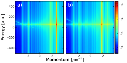
Figure 2: Logarithmic plot of the Rayleigh scattering spectrum of the two photon modes. The sample is excited by a spectrally narrow resonant laser pulse on either the symmetric (a), or anti-symmetric (b) branch. The correlation is $\mathcal{C}=0$, and the disorder potential is $V_{0}=0.1\,$meV, while the correlation length is $\xi=0.5\,\mu$m.

In Fig.3, we show the calculated far-field luminescence for three values of the disorder correlation (totally anti-correlated, $\mathcal{C}=-1$, uncorrelated, $\mathcal{C}=0$, and correlated $\mathcal{C}=1$), and for two different values of the pump momentum. In all six cases the pump is resonant with one of the polariton branches. Assuming cylindrically symmetric dispersions (isotropic effective masses), the Rayleigh rings should also be circular. The fact that they are skewed in the figures is a consequence of the periodic boundary conditions that we applied, but this will affect none of our conclusions.

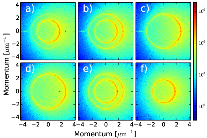
Figure 3: Logarithmic plot of the far-field emission power. The sample is excited by a spectrally narrow resonant laser pulse on either the anti-symmetric (a-c), or the symmetric (d-f) mode. The excitation momentum can be recognized as an intensity maximum at $\mathbf{k}=(2.8,0)$, and $\mathbf{k}=(1.9,0)\,\mu\mathrm{m}^{-1}$, respectively. The correlations of the disorder potential are $\mathcal{C}=-1$ (a, d), $\mathcal{C}=0$ (b, e), and $\mathcal{C}=1$ (c, f), while the transverse correlation length is $\xi=0.5\,\mu\mathrm{m}^{-1}$

There are a couple of general observations that we can make at this point. First, in all cases, the scattered intensity drops as a function of the distance from the pump position. This is a consequence of the finite transverse correlation length, and it has been observed experimentally, e.g., in Houdré et al. Houdré et al. (2000).

Second, for the totally anti-correlated disorder ($\mathcal{C}=-1$), intra-branch scattering is suppressed, and inter-branch scattering is maximum. The opposite is true for the case of totally correlated disorder ($\mathcal{C}=1$), while for uncorrelated disorder ($\mathcal{C}=0$), both inter-branch, and inter-branch scattering happens. This general trend is demonstrated more quantitatively in Fig. 4, where we plotted the amount of inter-, and intra-branch scattering as a function of the correlation, $\mathcal{C}$. As a measure of inter-branch scattering, we define the visibility-like quantities

$$v_{S}=\frac{{\displaystyle\int_{SS}}\,I(\mathbf{k})-{\displaystyle\int_{SA}}\,I(\mathbf{k})}{{\displaystyle\int_{SS}}\,I(\mathbf{k})+{\displaystyle\int_{SA}}\,I(\mathbf{k})}\,,\quad v_{A}=\frac{{\displaystyle\int_{AA}}\,I(\mathbf{k})-{\displaystyle\int_{AS}}\,I(\mathbf{k})}{{\displaystyle\int_{AA}}\,I(\mathbf{k})+{\displaystyle\int_{AS}}\,I(\mathbf{k})}$$ (9)

where the integration is over the pumped, or unpumped polariton branch. In the integrals, the first subscript designates the pumped branch, while the second subscript denotes the integration contour’s branch. Instead of using the ratio of the integrated intensities, the particular definition of $v_{A,B}$ is still normalized, but is devoid of the singularities that we would encounter when the scattering intensity tends to zero. Note that at this point, we did not stipulate the integration domain: depending on the experimental configuration, it could be the whole resonant circle, or, e.g., only half of it. (Experimentally, not the whole circle might be accessible, because the reflected light is usually masked.) The exact value of $v_{S,A}$ will, of course, depend on the integration domain, but the general trends will be unaffected. In order to account for the finite linewidth of the luminescence, and to average out statistical fluctuations, we integrate over a narrow circular shell of angular extent $2\pi$ and of radii $1.85-1.95$, and $2.75-2.85\,\mu\mathrm{m}^{-1}$, respectively. The pump region was excluded from the integration domain, so as to consider the scattered intensities only.

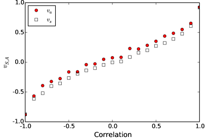
Figure 4: The dependence of the inter-branch scattering intensitiy on the transverse cross-correlation. The simulations parameters are the same as in Fig. 3, except for the correlation $\mathcal{C}$. The intensities are integrated over circular shells of radii $1.85-1.95$, and $2.75-2.85\,\mu\mathrm{m}^{-1}$, respectively. The transverse correlation length is $\xi=0.5\,\mu\mathrm{m}^{-1}$.

IV Analytical model

In this section, we will approach the problem from a different viewpoint: we assume that the disorder is weak, i.e., that plane waves are still approximate eigenstates of the Hamiltonian governing the evolution of photon modes, and the disorder is only a small perturbation. With these assumptions, scattering rates can be calculated using Fermi’s golden rule. Beyond the conceptual differences between this model (point-like scatterers) and the one that we discussed above (locally extended scatterers), the use of Fermi’s golden rule also implies that we neglect multiple scattering events. This should not come as a surprise, because Savona’s model is exact in the sense that we calculate the exact time evolution of the photon modes, i.e., we calculate to infinite order in the perturbation series, while Fermi’s golden rule truncates at the first order correction. However, for short times (short compared to the average scattering time) the differences should not be too large.

IV.1 Unperturbed eigenstates

Let us define the photon eigenvectors in the two cavities as

$$|\mathbf{k}_{a,b}\rangle=\varphi_{a,b}(z)e^{i\mathbf{k}\cdot\mathbf{r}}=|\varphi_{a,b}\rangle|\mathbf{k}\rangle\,.$$ (10)

As earlier, position vectors are understood in the plane of the cavities, and consequently, $\mathbf{k}$ is a two-dimensional wavevector. Given that the two cavities are spatially separated, $\varphi_{a}(z),\varphi_{b}(z)$ are not only orthogonal, but they have disjoint supports. When the disorder vanishes, the eigenstates of the coupled system are

$$|\mathbf{k}_{S,A}\rangle=\frac{1}{\sqrt{2}}\left(|\mathbf{k}_{a}\rangle\pm|\mathbf{k}_{b}\rangle\right)=\frac{1}{\sqrt{2}}(|\varphi_{a}\rangle\pm|\varphi_{b}\rangle)|\mathbf{k}\rangle\,.$$ (11)

Note that this decomposition into symmetric and anti-symmetric modes is valid only for the case of degenerate cavities. The generalization is straightforward, and it would not change the qualitative argument.

IV.2 Scattering matrix elements

Using the orthogonality of states located in spatially separated cavities, the scattering matrix element for intra-branch scattering of the symmetric branch can be written as

$$M_{\mathbf{k}\mathbf{k^{\prime}}}^{SS} = \langle\mathbf{k}_{A}|V_{a}(\mathbf{r})+V_{b}(\mathbf{r})|\mathbf{k^{\prime}}_{A}\rangle$$ (12)

$$= \frac{1}{2}(\langle\varphi_{a}|+\langle\varphi_{b}|)\langle\mathbf{k}|V_{a}(\mathbf{r})+V_{b}(\mathbf{r})|\mathbf{k^{\prime}}\rangle(|\varphi_{a}\rangle+|\varphi_{b}\rangle)$$

$$= \frac{1}{2}\langle\varphi_{a}|\varphi_{a}\rangle\langle\mathbf{k}|V_{a}(\mathbf{r})|\mathbf{k^{\prime}}\rangle+\frac{1}{2}\langle\varphi_{b}|\varphi_{b}\rangle\langle\mathbf{k}|V_{b}(\mathbf{r})|\mathbf{k^{\prime}}\rangle$$

$$= \frac{1}{2}\left[\tilde{V}_{\mathbf{k}-\mathbf{k^{\prime}}}^{a}+\tilde{V}_{\mathbf{k}-\mathbf{k^{\prime}}}^{b}\right]\,,$$

where $\tilde{V}_{\mathbf{q}}^{a,b}$ is the Fourier transform of the potentials. (In the matrix element $M_{\mathbf{k}\mathbf{k^{\prime}}}^{SS}$, the first superscript denotes the pumped mode at momentum $\mathbf{k}$, while the second superscipt is the mode to which the scattering happens at momentum $\mathbf{k^{\prime}}$.) The calculation for the anti-symmetric branch is similar, as are the results:

$$M_{\mathbf{k}\mathbf{k^{\prime}}}^{AA} = \frac{1}{2}(\langle\varphi_{a}|-\langle\varphi_{b}|)\langle\mathbf{k}|V_{a}(\mathbf{r})+V_{b}(\mathbf{r})|\mathbf{k^{\prime}}\rangle(|\varphi_{a}\rangle-|\varphi_{b}\rangle)$$ (13)

$$= \frac{1}{2}\left[\tilde{V}_{\mathbf{k}-\mathbf{k^{\prime}}}^{a}+\tilde{V}_{\mathbf{k}-\mathbf{k^{\prime}}}^{b}\right]\,.$$

From here we can draw the conclusion that the functional form of the scattering matrix element for intra-branch scattering is independent of whether the scattering happens on the symmetric or the anti-symmetric state (of course, the initial and final states on the two branches will correspond to wave vectors of different magnitude), and that it will be zero, if the Fourier coefficients of the two potentials are inverses of each other, i.e., when the potentials are totally anti-correlated. Note that this is a sufficient, but not a necessary condition.

Also note that these are only the matrix elements, but in order to calculate the transition probabilities, we still have to account for energy conservation. That requirement leads to the condition $|\mathbf{k}|=|\mathbf{k^{\prime}}|$.

Finally, we calculate the scattering matrix element for inter-branch scattering, and we obtain

$$M_{\mathbf{k}\mathbf{k^{\prime}}}^{SA} = \langle\mathbf{k}_{A}|V_{a}(\mathbf{r})+V_{b}(\mathbf{r})|\mathbf{k^{\prime}}_{B}\rangle$$ (14)

$$= \frac{1}{2}(\langle\varphi_{a}|+\langle\varphi_{b}|)\langle\mathbf{k}|V_{a}(\mathbf{r})+V_{b}(\mathbf{r})|\mathbf{k^{\prime}}\rangle(|\varphi_{a}\rangle-|\varphi_{b}\rangle)$$

$$= \frac{1}{2}\left[\tilde{V}_{\mathbf{k}-\mathbf{k^{\prime}}}^{a}-\tilde{V}_{\mathbf{k}-\mathbf{k^{\prime}}}^{b}\right]\,.$$

As for the other two cases, this expression gives only the scattering matrix elements, but energy conservation still has to be taken into account. We can also see that inter-branch scattering vanishes, whenever the disorder is totally correlated in the two cavities.

Another way of looking at this result is that, if both cavities have the same potential, then the system still possesses reflection symmetry with respect to the coupling mirror, and it still makes sense to talk about symmetric and anti-symmetric wavefunctions, and in such a case, scattering from one branch to the other is obviously forbidden by symmetry.

It is also worth pointing out that neither for inter-branch, nor for intra-branch scattering do the scattering rates depend explicitly on the strength of the coupling between the two cavities. The cavity splitting determines only the length of the momentum of the out-scattered polaritons, and thus the Fourier components that we have to consider for a particular pump angle. The scattering wavevectors are displayed in Fig. 5. The two cavities are pumped on either the symmetric branch ($S$) at at $\mathbf{k}=(2.2,0)\,\mu\mathrm{m^{-1}}$, or the anti-symmetric branch ($A$) at $\mathbf{k}=(1.2,0)\,\mu\mathrm{m^{-1}}$ (white dot), and scattering can happen to the wavevectors drawn by the dashed circles (red is the pumped, while green is the unpumped branch). These are the states whose energy is the same as that at the pump momentum. The difference wavevectors are depicted by the solid lines, and in order to find the scattering intensity on a particular branch, one has to integrate over one of these two circles.

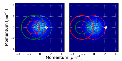
Figure 5: Rayleigh scattering in momentum space in a simple coupled cavity configuration. The white dot is the position of the pump beam ($\mathbf{k}=(1.2,0)\,\mu\mathrm{m^{-1}}$ on the left hand side, $\mathbf{k}=(2.2,0)\,\mu\mathrm{m^{-1}}$ on the right hand side), while the final states are drawn in dashed lines. The solid circles are the difference wavevectors that enter the matrix elements in Eqs. (12-14). In color scale, also shown is the Fourier transform of the disorder potential with a correlation length of $2\,\mu\mathrm{m}$.

IV.3 Scattering intensities

At this point, we can write the potentials as in Eqs. (7-8), and get for the Fourier transforms

$$\tilde{V}_{\mathbf{k}}^{a,b}=V_{0}\tilde{K}_{\mathbf{k}}(\xi)\tilde{N}_{\mathbf{k}}^{a,b}\,,$$ (15)

where $\tilde{K}_{\mathbf{k}}(\xi)$, and $\tilde{N_{\mathbf{k}}}^{a,b}$ are the Fourier transforms of the Gaussian kernel, and the random potential, respectively. Hence, the total scattering intensities from branch $i$ to branch $j$ are

$$I^{ij} \sim V_{0}^{2}\int\,d\mathbf{k}\left|\tilde{V}_{\mathbf{k}}^{a}\pm\tilde{V}_{\mathbf{k}}^{b}\right|^{2}=V_{0}^{2}\int\,d\mathbf{k}\tilde{K}_{\mathbf{k}}^{2}(\xi)\left|(1\pm\mathcal{C})\tilde{N}_{\mathbf{k}}^{a}\pm\sqrt{1-\mathcal{C}^{2}}\tilde{N}_{\mathbf{k}}^{b}\right|^{2}$$ (16)

$$= V_{0}^{2}\int\,d\mathbf{k}\tilde{K}_{\mathbf{k}}^{2}(\xi)\left\{(1\pm\mathcal{C})^{2}\left|\tilde{N}_{\mathbf{k}}^{a}\right|^{2}+\left(1-\mathcal{C}^{2}\right)\left|\tilde{N}_{\mathbf{k}}^{a}\right|^{2}\pm(1\pm\mathcal{C})\sqrt{1-\mathcal{C}^{2}}\left[\tilde{N}_{\mathbf{k}}^{a}(\tilde{N}_{\mathbf{k}}^{b})^{*}+(\tilde{N}_{\mathbf{k}}^{a})^{*}\tilde{N}_{\mathbf{k}}^{b}\right]\right\}$$

$$= V_{0}^{2}\int\,d\mathbf{k}\tilde{K}_{\mathbf{k}}^{2}(\xi)\left\{(1\pm\mathcal{C})^{2}\left|\tilde{N}_{\mathbf{k}}^{a}\right|^{2}+\left(1-\mathcal{C}^{2}\right)\left|\tilde{N}_{\mathbf{k}}^{a}\right|^{2}\right\}$$

$$= 2(1\pm\mathcal{C})V_{0}^{2}\int\,d\mathbf{k}\tilde{K}_{\mathbf{k}}^{2}(\xi)\left|\tilde{N}_{\mathbf{k}}^{a}\right|^{2}=2(1\pm\mathcal{C})V_{0}^{2}\mathcal{F}_{\pm}^{ij}\left(\left|\mathbf{k}_{\mathrm{in}}^{i}\right|,\left|\mathbf{k}_{\mathrm{out}}^{j}\right|,\xi\right)$$

because the cross-terms in the second line drop out, given that the two random variables are not correlated. We should point out that the intensity can be written in this simple form only when the disorder potential can be described by the same Gaussian kernel in the two cavities, i.e., when the transverse correlation lengths are identical. As in the numerical model, the integration is understood to be on a contour allowed by energy conservation, and the last line defines the function $\mathcal{F}_{\pm}^{ij}$, which measures the scattering amplitude. $\hbar\left|\mathbf{k}_{\mathrm{in}}^{i}\right|$, and $\hbar\left|\mathbf{k}_{\mathrm{out}}^{j}\right|$ are the length of the in-coming and out-scattered momenta. Therefore, the visibilities defined in Eq. (9) become

$$v_{S}=\frac{\left(\mathcal{F}_{+}^{SS}-\mathcal{F}_{-}^{SA}\right)+\mathcal{C}\left(\mathcal{F}_{+}^{SS}+\mathcal{F}_{-}^{SA}\right)}{\left(\mathcal{F}_{+}^{SS}+\mathcal{F}_{-}^{SA}\right)+\mathcal{C}\left(\mathcal{F}_{+}^{SS}-\mathcal{F}_{-}^{SA}\right)}=\frac{\gamma+\mathcal{C}}{1+\gamma\mathcal{C}}\,,$$ (17)

and

$$v_{A}=\frac{\left(\mathcal{F}_{+}^{AA}-\mathcal{F}_{-}^{AS}\right)+\mathcal{C}\left(\mathcal{F}_{+}^{AA}+\mathcal{F}_{-}^{AS}\right)}{\left(\mathcal{F}_{+}^{AA}+\mathcal{F}_{-}^{AS}\right)+\mathcal{C}\left(\mathcal{F}_{+}^{AA}-\mathcal{F}_{-}^{AS}\right)}=\frac{\mathcal{C}-\gamma^{\prime}}{1-\gamma^{\prime}\mathcal{C}}\,,$$ (18)

respectively. Here, we introduced the abbreviation

$$\gamma=\frac{\mathcal{F}_{+}^{SS}-\mathcal{F}_{-}^{SA}}{\mathcal{F}_{+}^{SS}+\mathcal{F}_{-}^{SA}}\,,\quad\mathrm{and}\quad\gamma^{\prime}=\frac{\mathcal{F}_{+}^{AA}-\mathcal{F}_{-}^{AS}}{\mathcal{F}_{+}^{AA}+\mathcal{F}_{-}^{AS}}\,.$$

We can make some general remarks even without explicitly calculating the scattering intensities. $v_{S,A}(\mathcal{C}=\pm 1)=\pm 1$, independent of the value of $\gamma,\gamma^{\prime}$ which only determine how the two endpoints are connected. Since, by definition, $\gamma,\gamma^{\prime}<1$, the curves behave in a strictly monotonic fashion as a function of $\mathcal{C}$. Also note that the two curves corresponding to the same value of $\gamma$, and $\gamma^{\prime}$ possess inversion symmetry around the origin, as can also be seen in Fig. (6).

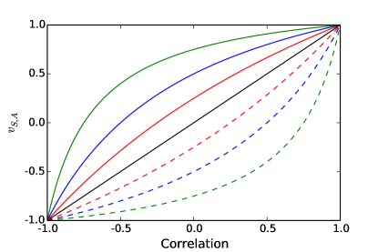
Figure 6: The curves $v_{S,A}$ as calculated from Eqs. (17-18) for $\gamma=0$ (black), $\gamma=1/4$ (red), $\gamma=1/2$ (blue), and $\gamma=3/4$ (green). The solid lines correspond to $v_{S}$ (Eq. (17)), while the dashed lines show $v_{A}$ (Eq. (18)).

IV.4 Special case: Gaussian correlations

There are further simplifications that we can make: since $N(\mathbf{r})$ is a random variable, so is $\tilde{N}_{\mathbf{k}}$, and we can then replace $|\tilde{N}_{\mathbf{k}}|^{2}$ by its average. If we do that, however, then $\mathcal{F}_{\pm}^{ij}$ becomes a contour integral over a Gaussian surface (the solid lines in Fig. 5), and we obtain

$$I^{ij} \sim \int e^{-|\mathbf{k}^{i}-\mathbf{k^{\prime}}^{j}|^{2}\xi^{2}}$$ (19)

$$= e^{-(k_{\mathrm{out}}^{2}+k_{\mathrm{in}}^{2})\xi^{2}}\int\,d\alpha e^{2k_{\mathrm{out}}k_{\mathrm{in}}\cos(\alpha)\xi^{2}}\,,$$

where $\alpha$ is the angle between the in-coming and out-going wavevectors. In the special cases, when the integration is over the $[0,2\pi]$ domain we get the modified Bessel function $I_{0}(2k_{\mathrm{out}}k_{\mathrm{in}}\xi^{2})$, and when it is over the $[\pi/2,3\pi/2]$ domain, the modified Struve function $L_{0}(2k_{\mathrm{out}}k_{\mathrm{in}}\xi^{2})$. It is also clear from the particular form in Eq. (19) that the relevant momentum scale is the inverse of the transverse correlation length.

Experimentally, it is probably hard to grow a sample with a prescribed transverse cross-correlation, and these correlations will also depend on the exact position on the sample. The transverse cross-correlation, therefore, is not a convenient control parameter. It does not mean, however, that the model cannot be tested. First, the very spatial variation can be exploited to realize different values of $\mathcal{C}$. Second, one can calculate the momentum dependence of the visibility at a fixed position, therefore, fixed correlation. The excitation energy fixes both the input and output wavevectors, and they can be calculated from the dispersion relations. In Fig. 7 we plot the visibility as a function of the excitation momentum for the experimentally realistic case of 14 meV mode splitting and cavity length $L=800$ nm, and for three different values of the transverse correlation length, $\xi$, with a transverse cross-correlation of $\mathcal{C}=0$. The integration domain was $[0,2\pi]$ (a), and $[\pi/2,3\pi/2]$ (b). Keeping in mind that in a reflection configuration the directly reflected light has to be blocked, the second domain is a more plausible experimental condition. The horizontal axis is always the shorter wavevector, i.e., $k^{*}=k_{\mathrm{in}}^{S}$ (pumping is on the symmetric branch), or $k^{*}=k_{\mathrm{out}}^{S}$ (pumping is on the anti-symmetric branch).

We can observe that independent of the transverse correlation length, the visibilities do not show a strong momentum dependence for case b). The physical reason for this is that (c.f. Fig. 5) the integration domain $[\pi/2,3\pi/2]$ samples the Gaussian kernel far from the center, where the function is relatively flat, but still decreasing. Therefore, by increasing the momentum, we integrate a slightly smaller integrand along a larger half circle, with the net result of obtaining approximately the same number. One would expect the same flat dependence from a simple filter theory, therefore, this measurement alone would not be able to distinguish between the various theories.

We can also notice that larger correlation lengths lead to larger absolute values for the visibilities. The interpretation of this is that for larger correlation lengths, the Gaussian kernel in momentum space is smaller, resulting in a more imbalanced intensity distribution on the two scattering circles. However, as the imbalance increases, so does the visibility.

As seen in Fig. 7a), when we integrate over the domain $[0,2\pi]$, the visibilities depend more strongly on the momentum. This can be understood, if we consider that in this case, the integration contour samples not only the flat, but the rapidly varying parts of the kernel, and it is no longer true that an increase in the length of the integration contour would be off set by the drop in the value of the kernel.

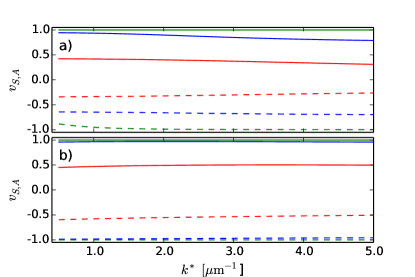
Figure 7: The dependence of the scattering visibility on the excitation momentum for three values of the transverse correlation length: $\xi=0.25$ (red) $0.5$ (blue), and $1\,\mu\mathrm{m}$ (green). The solid lines show $v_{S}$, while the dashed lines are $v_{A}$. The transverse cross-correlation was set to $\mathcal{C}=0$. The plot on the top shows curves for an integration domain of $[0,2\pi]$, and on the bottom $[\pi/2,3\pi/2]$.

V Conclusion

In conclusion, we have developed a theory for resonant Rayleigh scattering in coupled planar microcavity structures. In the first part of the paper, we extended Savona’s theory to the case of coupling, and presented some numerical results. This theory solves the exact time evolution of the photonic component of polariton scattering, and as such, is exact for all times. In the second part of the paper, we developed an analytical approach, and derived results. Given the perturbative nature of this model, these results can be trusted at short times only.

The main result of our paper is that depending on the transverse cross-correlations of the disorder potentials, RRS can be either enhanced, or suppressed on a particular polariton branch. Keeping an eye on parametric scattering schemes aiming to produce quantum correlated light, this result also means that it might be beneficial to use coupled cavities, even in the cases, where only a single polariton branch is involved, because if one can find a position on the sample, where the transverse cross-correlation is negative, then the relative strength of the parametric signal could be boosted on the branch under consideration.

Appendix A Scattering matrix elements in a triple cavity

Triple microcavities are used frequently in vertical (pump, signal and idler all are at zero momentum) parametric oscillators Diederichs and Tignon (2005); Diederichs et al. (2006); Diederichs et al. (2007a, b, c); Taj et al. (2009), or, as proposed in Portolan et al. Portolan2013, as a source of hyper-entangled photons. For this reason, we briefly discuss how the analytical model can be written down for such a case. When three identical cavities are pairwise coupled with equal couplings, the new eigenstates can be written as two completely symmetric, and a completely anti-symmetric linear combination of the original states:

$$|\mathbf{k}_{A}\rangle = \frac{1}{\sqrt{2}}(|\mathbf{k}_{a}\rangle-|\mathbf{k}_{c}\rangle)$$

$$|\mathbf{k}_{B}\rangle = \frac{1}{2}|\mathbf{k}_{a}\rangle-\frac{1}{\sqrt{2}}|\mathbf{k}_{b}\rangle+\frac{1}{2}|\mathbf{k}_{c}\rangle$$

$$|\mathbf{k}_{C}\rangle = \frac{1}{2}|\mathbf{k}_{a}\rangle+\frac{1}{\sqrt{2}}|\mathbf{k}_{b}\rangle+\frac{1}{2}|\mathbf{k}_{c}\rangle$$

The scattering matrix element can be calculated as in Eqs. (12-14), and we obtain the following results

$$M_{\mathbf{k}\mathbf{k^{\prime}}}^{AA} = \langle\mathbf{k}_{A}|V_{a}+V_{b}+V_{c}|\mathbf{k^{\prime}}_{A}\rangle=\frac{1}{2}(\tilde{V}_{\mathbf{k}-\mathbf{k^{\prime}}}^{a}+\tilde{V}_{\mathbf{k}-\mathbf{k^{\prime}}}^{c})$$

$$M_{\mathbf{k}\mathbf{k^{\prime}}}^{AB} = \langle\mathbf{k}_{A}|V_{a}+V_{b}+V_{c}|\mathbf{k^{\prime}}_{B}\rangle=\frac{1}{2\sqrt{2}}(\tilde{V}_{\mathbf{k}-\mathbf{k^{\prime}}}^{a}-\tilde{V}_{\mathbf{k}-\mathbf{k^{\prime}}}^{c})$$

$$M_{\mathbf{k}\mathbf{k^{\prime}}}^{AC} = \langle\mathbf{k}_{A}|V_{a}+V_{b}+V_{c}|\mathbf{k^{\prime}}_{C}\rangle=\frac{1}{2\sqrt{2}}(\tilde{V}_{\mathbf{k}-\mathbf{k^{\prime}}}^{a}+\tilde{V}_{\mathbf{k}-\mathbf{k^{\prime}}}^{c})$$

$$M_{\mathbf{k}\mathbf{k^{\prime}}}^{BB} = \langle\mathbf{k}_{B}|V_{a}+V_{b}+V_{c}|\mathbf{k^{\prime}}_{B}\rangle=\frac{1}{4}\tilde{V}_{\mathbf{k}-\mathbf{k^{\prime}}}^{a}+\frac{1}{2}\tilde{V}_{\mathbf{k}-\mathbf{k^{\prime}}}^{b}+\frac{1}{4}\tilde{V}_{\mathbf{k}-\mathbf{k^{\prime}}}^{c}$$

$$M_{\mathbf{k}\mathbf{k^{\prime}}}^{BC} = \langle\mathbf{k}_{B}|V_{a}+V_{b}+V_{c}|\mathbf{k^{\prime}}_{C}\rangle=\frac{1}{4}\tilde{V}_{\mathbf{k}-\mathbf{k^{\prime}}}^{a}-\frac{1}{2}\tilde{V}_{\mathbf{k}-\mathbf{k^{\prime}}}^{b}+\frac{1}{4}\tilde{V}_{\mathbf{k}-\mathbf{k^{\prime}}}^{c}$$

$$M_{\mathbf{k}\mathbf{k^{\prime}}}^{CC} = \langle\mathbf{k}_{C}|V_{a}+V_{b}+V_{c}|\mathbf{k^{\prime}}_{C}\rangle=\frac{1}{4}\tilde{V}_{\mathbf{k}-\mathbf{k^{\prime}}}^{a}+\frac{1}{2}\tilde{V}_{\mathbf{k}-\mathbf{k^{\prime}}}^{b}+\frac{1}{4}\tilde{V}_{\mathbf{k}-\mathbf{k^{\prime}}}^{c}$$

The potentials will be written as in Eqs. (7-8):

$$V_{a}(\mathbf{r}) = V_{0}\int\,d\mathbf{r^{\prime}}K(\mathbf{r},\mathbf{r^{\prime}},\xi)N_{a}(\mathbf{r^{\prime}})$$ (20)

$$V_{b}(\mathbf{r}) = \mathcal{C}_{a}V_{a}(\mathbf{r})+V_{0}\sqrt{1-\mathcal{C}_{a}^{2}}\int\,d\mathbf{r^{\prime}}K(\mathbf{r},\mathbf{r^{\prime}},\xi)N_{b}(\mathbf{r^{\prime}})$$ (21)

$$V_{c}(\mathbf{r}) = \mathcal{C}_{b}V_{b}(\mathbf{r})+V_{0}\sqrt{1-\mathcal{C}_{b}^{2}}\int\,d\mathbf{r^{\prime}}K(\mathbf{r},\mathbf{r^{\prime}},\xi)N_{c}(\mathbf{r^{\prime}})$$ (22)

or, in terms of the Fourier components,

$$\tilde{V}_{\mathbf{k}}^{a} = V_{0}\tilde{K}_{\mathbf{k}}(\xi)\tilde{N}_{\mathbf{k}}^{a}$$

$$\tilde{V}_{\mathbf{k}}^{b} = V_{0}\tilde{K}_{\mathbf{k}}(\xi)(\mathcal{C}_{a}\tilde{N}_{\mathbf{k}}^{a}+\sqrt{1-\mathcal{C}_{a}^{2}}\tilde{N}_{\mathbf{k}}^{b})$$

$$\tilde{V}_{\mathbf{k}}^{c} = V_{0}\tilde{K}_{\mathbf{k}}(\xi)(\mathcal{C}_{a}\mathcal{C}_{b}\tilde{N}_{\mathbf{k}}^{a}+\mathcal{C}_{b}\sqrt{1-\mathcal{C}_{a}^{2}}\tilde{N}_{\mathbf{k}}^{b}+\sqrt{1-\mathcal{C}_{b}^{2}}\tilde{N}_{\mathbf{k}}^{c})$$

and hence, the total scattered intensities can be expressed as

$$I^{AA} = \int\,d\mathbf{k}\left|M_{\mathbf{k}\mathbf{k^{\prime}}}^{AA}\right|{}^{2}=\frac{V_{0}^{2}}{4}\int\,d\mathbf{k}\tilde{K}_{\mathbf{k}}^{2}(\xi)\left|\tilde{V}_{\mathbf{k}}^{a}+\tilde{V}_{\mathbf{k}}^{c}\right|^{2}$$

$$= \frac{V_{0}^{2}}{4}\int\,d\mathbf{k}\tilde{K}_{\mathbf{k}}^{2}(\xi)\left\{(1+\mathcal{C}_{a}\mathcal{C}_{b})^{2}\left|\tilde{N}_{\mathbf{k}}^{a}\right|^{2}+\mathcal{C}_{b}^{2}(1-\mathcal{C}_{a}^{2})\left|\tilde{N}_{\mathbf{k}}^{b}\right|^{2}+(1-\mathcal{C}_{b}^{2})\left|\tilde{N}_{\mathbf{k}}^{c}\right|^{2}\right\}$$

$$= \frac{V_{0}^{2}}{4}\left[(1+\mathcal{C}_{a}\mathcal{C}_{b})^{2}+\mathcal{C}_{b}^{2}(1-\mathcal{C}_{a}^{2})+(1-\mathcal{C}_{b}^{2})\right]\int\,d\mathbf{k}\tilde{K}_{\mathbf{k}}^{2}(\xi)\left|\tilde{N}_{\mathbf{k}}^{a}\right|^{2}$$

$$= \frac{V_{0}^{2}}{4}\left[(1+\mathcal{C}_{a}\mathcal{C}_{b})^{2}+\mathcal{C}_{b}^{2}(1-\mathcal{C}_{a}^{2})+(1-\mathcal{C}_{b}^{2})\right]\mathcal{F}\left(\left|\mathbf{k}_{\mathrm{in}}^{A}\right|,\left|\mathbf{k}_{\mathrm{out}}^{A}\right|,\xi\right)$$

$$= \frac{V_{0}^{2}}{2}(1+\mathcal{C}_{a}\mathcal{C}_{b})\mathcal{F}\left(\left|\mathbf{k}_{\mathrm{in}}^{A}\right|,\left|\mathbf{k}_{\mathrm{out}}^{A}\right|,\xi\right)$$

because, due to the statistical independence of the noise distributions $\tilde{N}_{\mathbf{k}}^{a,b,c}$, all cross-terms vanish upon integration over a finite domain. All other intensites can be calculated in the same fashion, and we get

$$I^{AB} = \frac{V_{0}^{2}}{4}(1-\mathcal{C}_{a}\mathcal{C}_{b})\mathcal{F}\left(\left|\mathbf{k}_{\mathrm{in}}^{A}\right|,\left|\mathbf{k}_{\mathrm{out}}^{B}\right|,\xi\right)$$

$$I^{AC} = \frac{V_{0}^{2}}{4}(1+\mathcal{C}_{a}\mathcal{C}_{b})\mathcal{F}\left(\left|\mathbf{k}_{\mathrm{in}}^{A}\right|,\left|\mathbf{k}_{\mathrm{out}}^{C}\right|,\xi\right)$$

$$I^{BB} = \frac{V_{0}^{2}}{16}\left(6+\mathcal{C}_{a}^{2}\mathcal{C}_{b}^{2}+4\mathcal{C}_{b}\sqrt{1-\mathcal{C}_{a}^{2}}+2\mathcal{C}_{a}\left(2+\mathcal{C}_{b}+2\mathcal{C}_{a}\mathcal{C}_{b}\right)\right)\mathcal{F}\left(\left|\mathbf{k}_{\mathrm{in}}^{B}\right|,\left|\mathbf{k}_{\mathrm{out}}^{B}\right|,\xi\right)$$

$$I^{BC} = \frac{V_{0}^{2}}{16}\left(6+\mathcal{C}_{a}^{2}\mathcal{C}_{b}^{2}-4\mathcal{C}_{b}\sqrt{1-\mathcal{C}_{a}^{2}}-2\mathcal{C}_{a}\left(2-\mathcal{C}_{b}+2\mathcal{C}_{a}\mathcal{C}_{b}\right)\right)\mathcal{F}\left(\left|\mathbf{k}_{\mathrm{in}}^{B}\right|,\left|\mathbf{k}_{\mathrm{out}}^{C}\right|,\xi\right)$$

$$I^{CC} = \frac{V_{0}^{2}}{16}\left(6+\mathcal{C}_{a}^{2}\mathcal{C}_{b}^{2}+4\mathcal{C}_{b}\sqrt{1-\mathcal{C}_{a}^{2}}+2\mathcal{C}_{a}\left(2+\mathcal{C}_{b}+2\mathcal{C}_{a}\mathcal{C}_{b}\right)\right)\mathcal{F}\left(\left|\mathbf{k}_{\mathrm{in}}^{C}\right|,\left|\mathbf{k}_{\mathrm{out}}^{C}\right|,\xi\right)$$

The expressions for $I^{BA}$,$I^{CA}$, and $I^{CB}$ can be obtained by reversing the order of the arguments in $\mathcal{F}$:

$$I^{BA} = \frac{V_{0}^{2}}{4}(1-\mathcal{C}_{a}\mathcal{C}_{b})\mathcal{F}\left(\left|\mathbf{k}_{\mathrm{in}}^{B}\right|,\left|\mathbf{k}_{\mathrm{out}}^{A}\right|,\xi\right)$$

$$I^{CA} = \frac{V_{0}^{2}}{4}(1+\mathcal{C}_{a}\mathcal{C}_{b})\mathcal{F}\left(\left|\mathbf{k}_{\mathrm{in}}^{C}\right|,\left|\mathbf{k}_{\mathrm{out}}^{A}\right|,\xi\right)$$

$$I^{CB} = \frac{V_{0}^{2}}{16}\left(6+\mathcal{C}_{a}^{2}\mathcal{C}_{b}^{2}-4\mathcal{C}_{b}\sqrt{1-\mathcal{C}_{a}^{2}}-2\mathcal{C}_{a}\left(2-\mathcal{C}_{b}+2\mathcal{C}_{a}\mathcal{C}_{b}\right)\right)\mathcal{F}\left(\left|\mathbf{k}_{\mathrm{in}}^{C}\right|,\left|\mathbf{k}_{\mathrm{out}}^{B}\right|,\xi\right)$$

References

• Savona (2007) V. Savona, Journal of Physics: Condensed Matter 19, 295208 (2007).
• Carusotto and Ciuti (2004) I. Carusotto and C. Ciuti, Phys. Rev. Lett. 93, 166401 (2004), URL http://link.aps.org/doi/10.1103/PhysRevLett.93.166401.
• Christmann et al. (2012) G. Christmann, G. Tosi, N. Berloff, P. Tsotsis, P. Eldridge, Z. Hatzopoulos, P. Savvidis, and J. Baumberg, Phys. Rev. B 85, 235303 (2012), URL http://link.aps.org/doi/10.1103/PhysRevB.85.235303.
• Zajac et al. (2012) J. Zajac, E. Clarke, and W. Langbein, Appl. Phys. Lett. 101, 041114 (2012).
• Abbarchi et al. (2012) M. Abbarchi, C. Diederichs, L. Largeau, V. Ardizzone, O. Mauguin, T. Lecomte, A. Lemaitre, J. Bloch, P. Roussignol, and J. Tignon, Phys. Rev. B 85, 045316 (2012), URL http://link.aps.org/doi/10.1103/PhysRevB.85.045316.
• Houdré et al. (2000) R. Houdré, C. Weisbuch, R. Stanley, U. Oesterle, and M. Ilegems, Phys. Rev. B 61, R13333 (2000).
• Gurioli et al. (2001) M. Gurioli, F. Bogani, D. Wiersma, P. Roussignol, G. Cassabois, G. Khitrova, and H. Gibbs, Phys. Rev. B 64, 165309 (2001).
• Gurioli et al. (2002) M. Gurioli, F. Bogani, D. Wiersma, P. Roussignol, G. Cassabois, G. Khitrova, and H. Gibbs, physica status solidi a 190, 363–367 (2002).
• Gurioli et al. (2003) M. Gurioli, L. Cavigli, G. Khitrova, and H. Gibbs, Physica E 17, 463 (2003).
• Langbein (2004) W. Langbein, Journal of Physics: Condensed Matter 16, S3645 (2004).
• Langbein (2010) W. Langbein, La Rivista del Nuovo Cimento 33, 255 (2010).
• Zajac and Langbein (2012) J. Zajac and W. Langbein, arxiv p. arXiv:1208.0178v1 (2012).
• Freixanet et al. (1999) T. Freixanet, B. Sermage, J. Bloch, J. Marzin, and R. Planel, Phys. Rev. B 60, R8509 (1999).
• Sarchi et al. (2009) D. Sarchi, M. Wouters, and V. Savona, Phys. Rev. B 79, 165315 (2009), URL http://link.aps.org/doi/10.1103/PhysRevB.79.165315.
• Savona et al. (2000) V. Savona, E. Runge, and R. Zimmermann, Phys. Rev. B 62, R4805 (2000).
• Maragkou et al. (2011) M. Maragkou, C. Richards, T. Ostatnický, A. Grundy, J. Zajac, M. Hugues, W. Langbein, and P. Lagoudakis, Optics Letters 36, 1095 (2011).
• Einkemmer et al. (2013) L. Einkemmer, Z. Vörös, G. Weihs, and S. Portolan, arxiv p. 1305.1469 (2013), URL http://arxiv.org/abs/1305.1469.
• Diederichs and Tignon (2005) C. Diederichs and J. Tignon, Appl. Phys. Lett. 87, 251107 (2005).
• Diederichs et al. (2006) C. Diederichs, J. Tignon, G. Dasbach, C. Ciuti, A. Lemaître, J. Bloch, P. Roussignol, and C. Delalande, Nature 440, 904 (2006).
• Diederichs et al. (2007a) C. Diederichs, J. Tignon, G. Dasbach, C. Ciuti, A. Lemaître, J. Bloch, P. Roussignol, and C. Delalande (2007a).
• Diederichs et al. (2007b) C. Diederichs, J. Tignon, G. Dasbach, C. Ciuti, A. Lemaitre, J. Bloch, P. Roussignol, and C. Delalande, Superlattices and Microstructures 41, 301 (2007b).
• Diederichs et al. (2007c) C. Diederichs, D. Taj, T. Lecomte, C. Ciuti, P. Roussignol, C. Delalande, A. Lemaitre, L. Largeau, O. Mauguin, J. Bloch, et al., C. R. Physique 8, 1198 (2007c).
• Taj et al. (2009) D. Taj, T. Lecomte, C. Diederichs, P. Roussignol, C. Delalande, and J. Tignon, Phys. Rev. B 80, 081308R (2009).