Raster scan or 2-D approach?

We consider the relative merits of two different approaches to discovery or exclusion of new phenomena, a raster scan or a 2-dimensional approach.

1 Introduction

In this note, we consider two different types of method that can be applied in searches for new particles or new phenomena. An example would be the search for some hypothesised particle, such as the recently discovered Standard Model (S.M.) Higgs boson. For such a search, the data could be a mass histogram or the corresponding individual mass values, but more realistically would be augmented by other relevant kinematic variables. Then the aim is to try to distinguish between two hypotheses: that the data are due to some background processes ($H_{0}$), or that there is also the production of some new particle ($H_{1}$) . The former would result in some relatively smooth mass distribution, while the more exciting production of a new particle would produce a fairly sharp peak in mass spectra. We regard the new particle as being characterised by its mass $m_{H}$ and by its production cross-section $\sigma\$. We use this example through most of this note, but a couple of other situations involving new physics are discussed in Section 2.

We consider two possible approaches:

• Raster scan. Here we search over the physically interesting range of masses, and at each one separately we make a decision as to whether we can claim a discovery (i.e. decide that $H_{0}$ is excluded, and that $H_{1}$ is acceptable); exclude the existence of the new particle (reject $H_{1}$); or be unable to discriminate between them. This is done separately at each possible mass in the range, before moving on to the next mass - see Section 3.1.

• 2-D approach. A parameter-determination method is used for $m_{H}$ and $\sigma$, and the choice between $H_{0}$ and $H_{1}$ is based on the selected region in ($\sigma,m_{H}$) space - see Section 3.2.

It is to be noted that these two approaches use essentially the same data statistic $t$ (e.g. a likelihood ratio). The difference is that the 2-D approach looks for a 2-D region around the optimal values of $\sigma$ and $m_{H}$, while the raster scan determines a best region of $\sigma$ at each $m_{H}$ separately.

Our aim is to compare the relative merits of these two approaches.

2 Examples of Actual Searches

Here we mention briefly 3 examples of searches for new physics. Throughout this note, we use the language relevant for a Higgs search, but the ‘translation’ to our other two examples can be achieved via Table 1. These are not intended to be exact descriptions of the procedures used in actual searches, but more generic principles of approaches. For example, real searches for the Higgs boson involve several possible different decay modes; more data variables than just the mass $M$ for each event; uncertainties on energy scales, backgrounds and other systematics; etc.

• Higgs search.

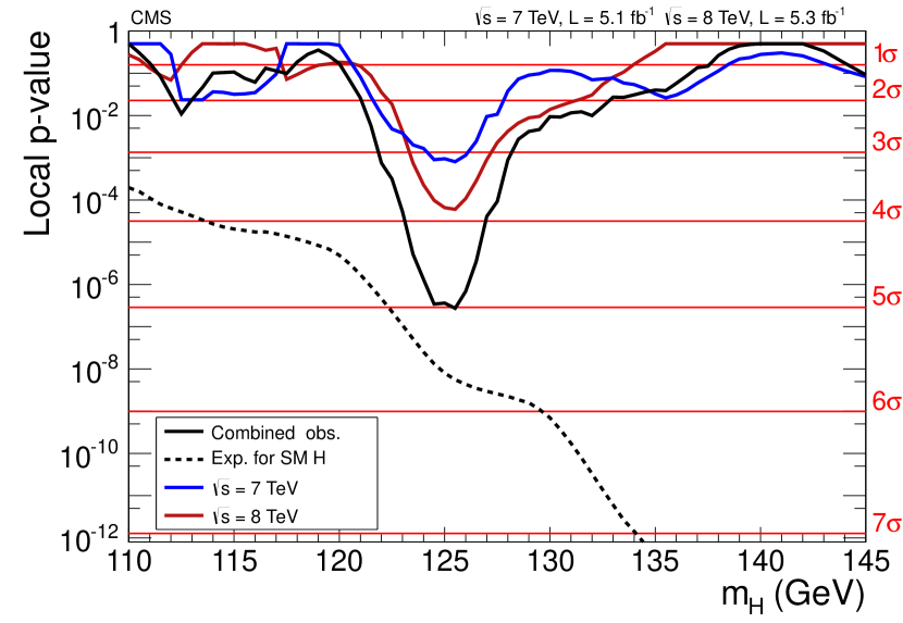
Figure 1: Search for the Higgs boson. The plot from ref. [1] shows the local $p$-value for the null hypothesis (‘No Higgs in data, but just Standard Model background’) as a function of the supposed mass of the Higgs $m_{H}$. The three solid curves show the $p$-values for the 7 TeV data, for the 8 TeV data available at the time, and for their combination. The dashed curve is the expected $p$-value for the combined data, assuming the Higgs exists and is produced and decays as predicted by the S. M., also as a function of $m_{H}$. The fact that in the vicinity of 125 GeV the combined $p$-value reaches a value below $10^{-6}$, equivalent to a $\sim 5\sigma$ tail of a Gaussian distribution, and is in satisfactory agreement with the expected $p$-value, is taken as evidence of the discovery of a particle, consistent with the expected properties of a Higgs boson.

  This was performed using a raster scan [1, 2]. At each closely spaced mass over the relevant range, a separate search was performed. Fig. 1 shows the $p$-values for the null hypothesis as a function of $m_{H}$. Based on this (and on a comparison of $\sigma$ with the Standard Model prediction, as well as branching ratios for various decay modes), the discovery of a Higgs particle with mass around 126 GeV was claimed.

• $B_{s}$ oscillations[3, 4].

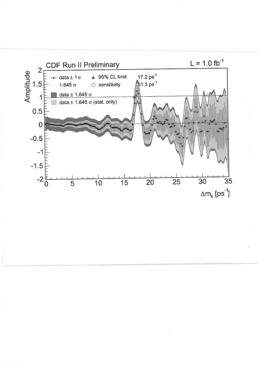
Figure 2: Fit of $B_{s}$ oscillations to data from the CDF experiment[3] at Fermilab’s Tevatron. A raster scan is performed at each $\Delta m_{s}$, the mass difference between the $B_{s}$ and its antiparticle, to extract the amplitude $A$ of the oscillations at that frequency. The evidence for oscillations is that for $\Delta m_{s}$ near 17 $ps^{-1}$, $A$ is very far from zero, but is consistent with the oscillations’ expected value of unity.

  These are parametrised by the amplitude $A$ of oscillations and their frequency, which is proportional to the mass difference $\Delta m_{s}$ between the $B_{s}$ and its anti-particle. A raster scan was performed to determine $A$ at each mass difference $\Delta m_{s}$ - see fig. 2. If such oscillations occur, the value of $A$ should be unity at the relevant $\Delta m_{s}$, whereas otherwise $A$ is expected to be close to zero. On the basis of the data, the discovery of $B_{s}$ oscillations at a mass difference of $\sim 17ps^{-1}$ was claimed.

• Neutrino oscillations.

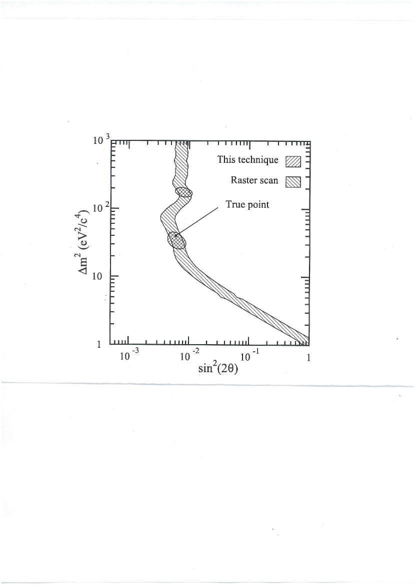
Figure 3: Search for neutrino oscilllations, parametrised by $\sin^{2}(2\theta)$ and $\Delta m^{2}$. The simulated ‘data’ were generated assuming the parameter values denoted by ‘True point’. The single hatched band is the result of a raster scan in which the best fit region in $\sin^{2}(2\theta)$ is determined for each value of $\Delta m^{2}$. The double hatched region is the result of determining the parameters in a 2-D fit, using the Feldman-Cousins approach[5]; the plot is taken from their paper.

  In a simplified model with only two species of mixing neutrinos, their oscillations are specified by an amplitude $\sin^{2}(2\theta)$ and by their frequency which is proportional to $\Delta m^{2}$, the difference in mass squared of the two neutrino types. A given set of data can be analysed by obtaining the best value of $\sin^{2}(2\theta)$ at each value of $\Delta m^{2}$ (i.e. a raster scan), and seeing whether sin${}^{2}(2\theta)\,=\,0$ is excluded. However, Feldman and Cousins[5] point out that for extracting $(\sin^{2}(2\theta),\Delta m^{2})$ a 2-D parameter determination is preferable (see Fig 3).

Table 1: Examples of searches for new physics, characterised by a strength $\phi_{1}$ and a mass parameter $\phi_{2}$.

Data and params	Event variables	Strength $\phi_{1}$	Mass param $\phi_{2}$
Example
Higgs	Mass $M$	Cross-section $\sigma$	Mass $m_{H}$
$B_{s}$ oscillations	Length, energy, decay mode	Amplitude $A$	Mass diff $\Delta m_{s}$
$\nu$ oscillations	Length, energy, interaction type	Amplitude $\sin^{2}(2\theta)$	Diff in mass-sq $\Delta m^{2}$

An interesting question is why the search for $B_{s}$ oscillations uses a raster scan, but for neutrino oscillations a 2-D approach is used. The main reason is that the emphasis of the analysis in the neutrino oscillation case was to determine the values of the parameters $\sin^{2}(2\theta)$ and $\Delta m^{2}$, while in the $B_{s}$ case it was whether the $B_{s}$ oscillations could be discovered. Also the amplitude in the $B_{s}$ case is expected to be unity, while for the neutrinos any value from zero to unity is physically possible.

Another interesting contast between searches for these two types of oscillations is the difference in the appearence of the raster scan in the two cases. At small mass differences, the raster scan for $B_{s}$ gives values of the amplitude close to zero. In contrast, the neutrino oscillation amplitude in the corresponding region can be large. The reason is that the range of observable times in the $B_{s}$ case covers several complete oscillations, while for some neutrino experiments, only a small part of the first oscillation can be observed. Thus the $B_{s}$ data tend to pick out the correct oscillation frequency, with the fitted amplitude at smaller frequencies being close to zero; while neutrino experiments in this regime are sensitive essentially only to the product $\ sin^{2}(2\theta)\times(\Delta m^{2})^{2}$, so smaller $\Delta m^{2}$ values need a larger amplitude.

3 Further Details

There are several possible choices for the way a preferred region in parameter space is defined, whether this is for just $\sigma$ for the raster scan, or for both $m_{H}$ and $\sigma$ for the 2-D approach. A partial list of possible methods is:

• Maximum likelihood approach, with the selected region being those parameter values for which

  $$\Delta ln{\calligra L}\ =\ ln{\calligra L}_{max}-ln{\calligra L}(\sigma,m_{H})\leq C,$$ (1)

  where $ln{\calligra L}(\sigma,m_{H})$ is the logarithm of the likelihood for parameter values $(\sigma,m_{H})$; ${\calligra L}_{max}$ is the maximum of the likelihood as a function of $\sigma$ for the Raster Scan, or of both $\sigma$ and $m_{H}$ for the 2-D approach; and $C$ is a constant whose value depends on the desired nominal coverage level and on the number of free parameters. For example, for a $95\%$ region in a 1 or 2 parameter problem, $C$ would be 1.9 or 3.0 respectively.

• An alternative but related approach would be to define a $\chi^{2}$ region such that $\chi^{2}(\sigma,m_{H})-\chi^{2}_{best}$ is below some critical value.

• Frequentist approach. This uses the Neyman construction, with parameter(s) $\mu$ as $\sigma$ for the raster scan, or ($\sigma,m_{H}$) for the 2-D approach. For each value of $\mu$, the probability density for observing possible data $d$ is used in conjunction with an ordering rule to construct the confidence band containing the likely range of data values for the given $\mu$, at the chosen confidence level. The observed data are then used to determine the range of parameter values for which the data is likely.

  With just one parameter, the ordering rule can be chosen to provide upper or lower limits, or central regions (e.g. equal tail probabilities).

  In the Feldman-Cousins version of the frequentist approach, a likelihood-ratio is used to define the ordering rule. This extends naturally to situations with more than one parameter. The Feldman-Cousins approach is called ‘unified’ as, depending on the data, the pre-defined ordering rule determines whether the 1-D preferred region will be single-sided (i.e. an upper or a lower limit), or double-sided.

  Another feature of the Feldman-Cousins method is that, in contrast to the frequentist approach with other ordering rules, empty intervals or those consisting just of the point $\sigma=0$ are far less likely.

• Bayesian methods. Here the likelihood function is multiplied by the prior probability density $\pi({\sigma,m_{H}})$ to obtain the posterior probability density $p({\sigma,m_{H}})$. From this, a region can be selected in parameter space that contains the required level $f_{Bayes}$ of integrated posterior probability density. As always the Bayesian approach requires the specification of the (possibly multi-dimensional) prior, and it is advisable to perform a sensitivity analysis to see how much the result depends on the choice of prior.

  If there is only one parameter, even for a given $f_{Bayes}$, the region could be chosen for an upper limit, lower limit, central interval with equal probability in each tail, shortest interval, etc.

  With more than one parameter, the obvious choice is to use a cut on the value of the posterior probability density, which in one dimension corresponds to the minimum length interval. Again this produces regions which are not invariant with respect to reparametrisations of $(\sigma,m_{H})$. There is no such problem for the likelihood, $\chi^{2}$ or Feldman-Cousins approaches.

Frequentist methods have the advantage over other approaches that coverage is guaranteed i.e. the procedure is such that for a series of repeated analyses each with new data, in the absence of experimental biases, the fraction of times that the true value of the parameter(s) will be contained within the preferred region will be at least that specified by the chosen confidence level.

In this note, we use the generic name ‘preferred region’ for the 1-D or 2-D parameter regions produced by any of these methods. Clearly, any test to see whether $\sigma$ is consistent with zero cannot employ a lower or an upper limit technique; equi-tailed central intervals may be problematic too.

3.1 Raster Scan

3.1.1 Procedure

The characteristic of a raster scan is that it is performed at each mass $m_{H}$ separately, and independently of what happens at any other mass. At each such mass, a decision is made to exclude $H_{1}$, to reject the null hypothesis $H_{0}$ or to make no choice. Thus at each mass $m_{H}$, a region of $\sigma$ is determined at the pre-defined confidence level, even though the overall fit to the data using these parameters may be much worse than fits at other masses; the raster scan ignores the fact that there may be a discrepancy, and still provides a range for $\sigma$ at each mass. It then checks whether these regions contain zero (as a test of the null hypothesis $H_{0}$) or/and $\sigma_{SM}$, the predicted cross-section assuming S.M. Higgs. If the region excludes $\sigma=0$, then $H_{0}$ is excluded at the relevant confidence level, while if it does not contain $\sigma_{SM}$, the predicted cross-section, then $H_{1}$ is excluded. It is thus possible to claim a discovery of the Higgs at a specific mass; to claim discoveries at more than one mass; to exclude the S.M. Higgs over a range of masses; to have insufficient evidence for choosing between $H_{0}$ and $H_{1}$; or a combination of these.

An analogous procedure is used in the search for $B_{s}$ oscillations, where the amplitude $A$ is determined at each $\Delta m_{s}$.

Of course, a lot of detail has been ignored in the above brief description. Further discussion of hypothesis testing techniques, including the so-called $CL_{s}$ method[6] for excluding $H_{1}$, can be found in ref. [7].

3.1.2 Features

• We have already mentioned that because the raster scan treats each mass separately, the conclusion as to what the data tell us at one mass is completely unaffected by what is happening at other masses (Contrast the 2-D approach below.)

• Another consequence of dealing with each mass separately is that it may be possible to claim discoveries of more than one ‘S.M.’ Higgs.

• The raster scan will provide a cross-section range for each mass, regardless of the quality of the fit.

• The prefered region defined by the raster scan for $\sigma$ at each possible $m_{H}$ is different from what would have been obtaind by determining the $m_{H}$ range at each $\sigma$. In the case of the Higgs (and $B_{s}$) searches, the former is used as it is more physically motivated, and it works better in practice; this might not be the case in different sorts of analyses where the two parameters might have a more symmetric status.

3.2 2-D Parameter Determination

3.2.1 Procedure

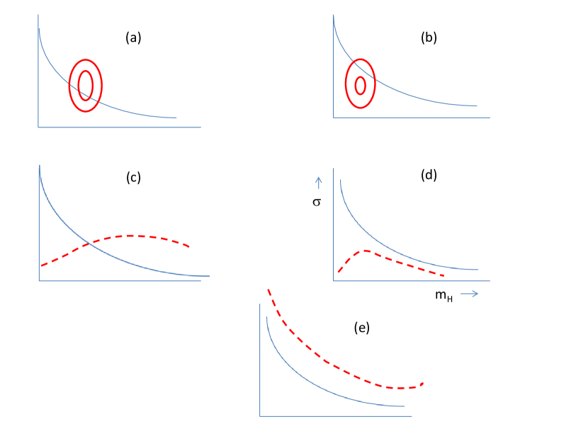
Figure 4: Some possible preferred regions in parameter space in a method of determining the two physics parameters $\sigma$ and $m_{H}$ simultaneously. The solid curve is the predicted cross-section $\sigma$ at each mass, according to the Standard Model. The $\sigma=0$ axis is a contour line at some acceptance level, since with zero production rate, the mass is irrelevant. (a) The smaller ellipse is a 95% CL region, and the larger one corresponds to 5$\sigma$. Since the larger ellipse does not reach down to the $\sigma=0$ axis, this corresponds to a discovery claim, with masses outside the smaller ellipse being excluded. (b) Although the 5$\sigma$ ellipse excludes a zero cross-section, the 95% CL one does not include the predicted cross-section, and so the hypothesised particle is excluded at all masses. This could be due to the production of a new particle, but at a lower rate than predicted by theory. (c) The dashed line shows the upper limit of the 95% confidence region. For masses below the cross-over between the upper limits and the theoretical curve, the existence of the hypothesised particle is excluded; for higher masses, the data does not distinguish between the two hypotheses $H_{1}$ and $H_{0}$. (d) The 95% CL region is below the predicted cross-section at all masses, and so the hypothesised new particle is excluded. (e) The upper edge of the 95% CL region lies above the predicted cross-section at all masses, and so the data does not distinguish between existence or not of the new particle.

As a result of a 2-D search for the preferred region at some level (see Fig 4, where some possibilities are shown), some rules have to be formulated for deciding whether we can claim a discovery; exclude/disfavour the existence at some or perhaps even all relevant masses; or be unable to distinguish between these possibilities.

Even apart from the choice of confidence levels, there is some degree of arbitrariness in how the procedure is defined. We consider the following as an example of a possible set of rules:

• Discovery: We require the 2-D preferred region at the 5$\sigma$ level to exclude $\sigma=0$; and also require the predicted $\sigma_{SM}$ to be within the 95% contour. This ensures that the observed signal strength is as expected; a consequence of this is that an apparent signal which is significantly smaller or larger than predicted does not count as a discovery.

  It may also be reasonable to impose a requirement that the width in $m_{H}$ of the discovery region be consistent with expectation. e.g. in a channel with good mass resolution such as $H\rightarrow\gamma\gamma$ or $H\rightarrow ZZ\rightarrow 4$ charged leptons, an apparent signal over a very wide mass region may be more likely to correspond to a mis-modeled background than to a fundamental discovery. (This applies also to raster scans.)

• Exclusion: Masses at which the 95% region does not include $m_{H}$ are excluded. This includes the case where the single S.M. Higgs boson has been discovered at some other mass.

• No decision: This applies when the 95% region includes both $\sigma=0$ and $\sigma=\sigma_{SM}$, unless the Higgs boson has been discovered at some other mass.

3.2.2 Features

• Usually when we quote the mass uncertainty on a new particle state, this is interpreted as a 1$\sigma$ error region. In the 2-D approach, the discovery region is defined by a 5$\sigma$ contour, which will usually correspond to a wider mass interval. This is not a big problem as, once the existence of the particle is established, its mass could be determined in a separate analysis using any desired criterion for defining the mass uncertainty.

• Because the model used for analysing the data assumes that there is only one S. M. Higgs boson, a signal at one mass ($m_{1}$) affects what happens at other masses. Thus if there is another mass $m_{2}$ which in a raster scan also shows a 5$\sigma$ signal, $m_{2}$ could appear in the exclusion region in the 2-D approach if the signal at $m_{1}$ has larger significance. Similarly, because of discovery of the one and only Higgs boson at $m_{1}$, other masses are excluded; this includes mass regions where the experimental data has only very weak (or even no) discrimination to the presence or absence of a Higgs boson.

  Thus the 2-D approach with the assumption of just one Higgs boson has a higher probability than the raster scan has of excluding the Higgs at other masses. However, in the absence of a significant excess throughout the mass range, the exclusion power of the raster scan is better, largely because of the higher cut on the log-likelihood ratio needed in the 2-D scenario[8].

• Similarly for discovery at the favoured mass, the 2-D $5\sigma$ region will include a wider range of cross-section (and hence be less sensitive to discovery) than the corresponding region in a raster scan. For a frequentist method such as Feldman-Cousins, the $p$-values for excluding zero cross-section will be global and local (for the 2-D and raster scan approaches respectively).

• There are other situations in which the above procedure is not logical. For example, the preferred region might correspond to a low or a high signal rate, such that it does not qualify as a discovery claim, and yet we still exclude all other masses outside the preferred region, even including those where we have little or no sensitivity.

3.3 Absence of predicted signal strength

In some searches for the New Physics embodied in the alternative hypothesis $H_{1}$, there might not be a prediction for the signal strength. For example, the strength of gravitational waves observed on Earth depends on various parameters of the source, including its distance from us. Similarly with neutrino oscillations, the strength factor $\sin^{2}(2\theta)$ can take on any value between zero and 1. In such situations, the procedures for exclusion of $H_{1}$ (and to some extent, its discovery too) are modified.

3.3.1 Raster Scan

Because we deal with each mass separately, we can make a discovery by finding that the strength factor is inconsistent with zero. (Indeed it may be that this happens at more than one mass.) However, no check is possible that the strength is consistent with expectation, as the latter does not exist.

In contrast, there can be no excluded mass region, basically because the phenomenon could have a very weak strength, below the sensitivity of the experiment. It is possible, however, to produce an upper limit on the possible strength at each mass, which can then be built up into an exclusion region in (strength, mass) parameter space.

3.3.2 2-D approach

After the preferred region is found in 2-D parameter space, we can make the usual discovery claims, except that as in the raster scan, there is no possible check that the strength of the observed effect is as expected.

However, we now can have excluded mass regions, being those that lie outside the preferred region. This is possible even without a predicted signal strength, provided $H_{1}$ involves the assumption that there is only one true set of values for the parameters.

4 Conclusions

Table 2 contains an overview of various features of the raster scan and 2-D approaches to discovery and exclusion. A few comments about some of the entries are worth emphasising.

Table 2: Relative merits of Raster Scan and 2-D approach

Method	Raster Scan	2-D
Features
Aim	Determines $\sigma$ region at each $m_{H}$	Determines $(\sigma,m_{H})$ region
Discovery criterion	$\sigma$ region excludes 0	2-D region excludes $\sigma=0$
Multiple discoveries possible?	Yes	No
Discovery at $m_{1}$ affects other $m$?	No	Yes
Exclusion criterion	$p$ or $CL_{s}$ <5%	Region excludes $\sigma=\sigma_{SM}$
Exclusion at $m_{1}$ affects other $m$?	No	No
Possible to exclude at $m$ with no sensitivity?	No	Yes
Confidence levels	Separate for discovery, exclusion. Measure $m$ separately	Different for discovery, exclusion, measurement of $m$
Local or global $p$?	Local. Needs LEE for global	Global
Good points	Treats each mass separately.                 Better sensitivity	Regions with poor Goodness of Fit not accepted
Bad points	Determines $\sigma$ at $m$ where fit is poor. Raster in $m$ different from in $\sigma$	Can exclude where no sensitivity
Method best for…	Hypothesis testing	Parameter determination

The fundamental difference between the two methods is that the 2-D approach assumes that there is (at most) one S.M. Higgs boson, while the raster scan is more flexible in that it treats each mass separately. This then can result in the 2-D method excluding Higgs production at masses for which there is essentially no sensitivity to Higgs production, simply because a discovery claim is made at another mass. Another consequence is that part of the preferred region in $(\sigma,m_{H})$ space from the raster scan can correspond to very poor fits of the theory to the data; in the 2-D approach, only the best fit region is obtained.

Both methods use separate confidence levels for searches and for exclusion. When a discovery is claimed at the 5$\sigma$ level, the 2-D approach provides a mass region over which this occurs. However a mass measurement should be performed separately as this traditionally uses a 68% confidence level for the uncertainty. In the raster scan, the mass measurement is clearly a separate exercise from the Hypothesis Testing of discovery.

To associate a $p$-value with a discovery claim, we need to determine the (hopefully very low) probability of a background fluctuation giving rise to an effect at least as large as the one observed. If a frequentist approach is used to determine the preferred regions, the $p$-value for a discovery claim is directly determined by the method, as coverage is guaranteed; otherwise a brute-force Monte Carlo approach may be needed.

There are (at least) two $p$-values to consider: the local one, which is the probability of such a fluctuation at the mass observed for the data signal, and a global $p$-value which incorporates the Look Elsewhere Effect (LEE)[9] i.e. the chance of having such a fluctuation not only at the observed mass, but anywhere in the analysis. The 2-D approach most naturally lends itself to calculating the global $p$-value over the range of masses relevant for the analysis, while in the raster scan the local $p$-value is more easily calculated, and hence needs to be corrected for the LEE.

In conclusion, it appears that the raster scan provides a more natural approach to discovery or exclusion of New Physics, while the 2-D approach is preferable for parameter determination.

I would like to thank Bob Cousins, Jon Hays, Tom Junk, Richard Lockhart, Yoshi Uchida, Nick Wardle, Daniel Whiteson and members of the CMS Statistics Committee for many useful discussions and patient explanations.

References

- [1] S. Chatrchyan et al., CMS Collaboration, Phys. Lett. B716 (2012) 30
- [2] G. Aad et al., ATLAS Collaboration, Phys. Lett. B716 (2012) 1
- [3] A. Abulencia et al., CDF Collaboration, Phys. Rev. Lett. 97 (2006) 242003
- [4] V. M. Abazov et al., D0 Collaboration, Phys. Rev. Lett. 97 (2006) 021802
- [5] G. J. Feldman and R. D. Cousins, Phys. Rev. D57 (1998) 3873
- [6] A. Read, ‘Modified frequentist analysis of search results’, Workshop on Confidence Limits, CERN Yellow Report 2000-05, p81; and ‘Presentation of search results - the method’, Advanced Statistical Techniques in Particle Physics, Durham IPPP/02/39 (2002) p11.
- [7] L. Lyons, ‘Methods for comparing two hypotheses’, http://www.physics.ox.ac.uk/users/lyons/H0H1_June23_09.pdf
- [8] CDF Collaboration ‘Search for High Mass Resonances Decaying to Muon Pairs in TeV Collisions’ (2011) http://arxiv.org/abs/arXiv:1101.4578
- [9] L. Lyons, ‘Comments on Look Elsewhere Effect’, www.physics.ox.ac.uk/users/lyons/LEE_feb7_2010.pdf