Overlapping Trace Norms in Multi-View Learning

Abstract

Multi-view learning leverages correlations between different sources of data to make predictions in one view based on observations in another view. A popular approach is to assume that, both, the correlations between the views and the view-specific covariances have a low-rank structure, leading to inter-battery factor analysis, a model closely related to canonical correlation analysis. We propose a convex relaxation of this model using structured norm regularization. Further, we extend the convex formulation to a robust version by adding an $\ell_{1}$-penalized matrix to our estimator, similarly to convex robust PCA. We develop and compare scalable algorithms for several convex multi-view models. We show experimentally that the view-specific correlations are improving data imputation performances, as well as labeling accuracy in real-world multi-label prediction tasks.

Keywords: CCA, Multi-view, Convexity, PCA, ADMM

1 Introduction

Canonical correlation analysis (CCA) was first introduced by Hotelling (1936) to analyse the linear relationship between a pair of random vectors. Similar to principal component analysis (PCA) Jolliffe (1986), which finds for a random vector a basis in which the covariance matrix is diagonal and the variances on the diagonal are maximized, CCA finds two bases in which the correlation matrix between the variables is diagonal and the correlations on the diagonal are maximized. The principal directions in PCA span a subspace in which the observations can be projected with minimum reconstruction error (when defined in terms of sum of squares), while the canonical directions span a pair of subspaces in which the co-occurring observations are maximally aligned after projection. CCA and its extensions are widely used in multivariate statistics and machine learning and have found applications in image processing Borga (1998), biology Parkhomenko et al. (2009) and geophysics Cannon and Hsieh (2008).

An important limitation of CCA is that it is only able to capture linear dependencies between two data sets. In order to capture nonlinear alignments, kernel CCA was introduced Bach and Jordan (2002); Hardoon et al. (2004). In this setting, the data sets are projected into high-dimensional feature spaces, where a perfect alignment can always be recovered if the dimension of the feature spaces is sufficiently large. Another line of research was triggered by the probabilistic reformulation of CCA by Bach and Jordan (2005), which in turn led to robust Archambeau et al. (2006) and sparse extensions Archambeau and Bach (2008); Jia et al. (2010).

Probabilistic CCA assumes that the pair of high-dimensional random vectors are coupled by a shared low-dimensional latent vector, which captures the correlations between the two realisations. It provides a natural framework for generalizing CCA to multiple co-occurring data sets, often called views, and for accounting for view-specific variations by augmenting CCA with view-specific low-dimensional latent vectors able to capture the residual covariance in each view. These two variants have often been loosely called CCA by the machine learning community. An example of the former to support text categorisation in the presence of multi-lingual documents is proposed by Amini et al. (2010). The latter is known as inter-battery factor analysis (IBFA) Tucker (1958); Klami et al. (2013) in the statistics literature. The main challenge with IBFA is the identifiability of view-specific and shared variations. This problem was elegantly addressed by Virtanen et al. (2011); Klami et al. (2013) by proposing a Bayesian treatment of IBFA, involving group sparsity and on automatic relevance determination MacKay (1996) to infer the dimension of the latent vectors (shared and view-specific) without having to resort too expensive cross-validation.

Recently, convex formulations of multi-view learning were also proposed Goldberg et al. (2010); White et al. (2012); Christoudias et al. (2012); Cabral et al. (2011), extending recent work done on matrix completion, often justified as convex relaxation of low-rank recovery problems through the nuclear norm Candès and Recht (2009). To the best of our knowledge, none of the existing convex multi-view approaches consider the view-specific variations as part of their model. In some settings the view-specific covariances could be diagonalized beforehand, but this normalization step, known as whitening, can be computationally expensive in high dimension and it is not straightforward in the presence of missing values. Moreover, a whitening pre-processing step would not take into account possible linear dependencies between the two data sets and would thus be suboptimal.

We present a convex relaxation of IBFA in the presence of missing values, which can straightforwardly be generalized to its multi-view version and which can deal with continuous and discrete data. The core idea of our approach is to include a nuclear norm penalty in the objective function for each view to capture the view-specific covariances, along with a shared nuclear norm penalty to capture the correlations between the views. We further extend our approach to the robust PCA framework of Candès et al. (2011) to account for atypical observations such as outliers.

The paper is organized as follows. Section 2 introduces the convex objective for IBFA as a convex relaxation of the standard probabilistic model. In Section 3, we describe an efficient algorithm to minimize the objective, using the Alternating Direction Method of Multipliers (ADMM)l. In Section 4, we evaluate the model on a wide variety of data sets, and compare our proposed ADMM algorithm to several off-the-shelf SDP solvers.

2 Convex formulations of multi-view matrix completion

Let $\{(y_{1i},y_{2i}):y_{1i}\in\mathbb{R}^{d_{1}},y_{2i}\in\mathbb{R}^{d_{2}}\}_{i=1}^{n}$ be co-occurring data pairs. The number of features in view 1 and 2 are respectively denoted by $d_{1}$ and $d_{2}$. The main reason for defining two vectors of observations rather than a single concatenated vector in the product space $\mathbb{R}^{d_{1}+d_{2}}$ is that the nature of the data in each view might be different. For example, in a multi-lingual text application, the views would represent the features associated with two distinct languages. Another example is image labeling, where the first view would correspond to the image signature features and the second view would encode the image labels. In the remainder, we will restrict our discussion to two views for clarity of the presentation, but the extension to an arbitrary number of views is straightforward.

2.1 Overlapping nuclear norms

We stack the observations $\{y_{1i}\}_{i=1}^{n}$ and $\{y_{2i}\}_{i=1}^{n}$ respectively into the matrices $Y_{1}:=\{y_{1ij}\}\in\mathbb{R}^{d_{1}\times n}$ and $Y_{2}:=\{y_{2ij}\}\in\mathbb{R}^{d_{2}\times n}$. To compare different multi-view approaches, we will consider predictive tasks, where the goal is to predict missing elements in matrices $Y_{1}$ and $Y_{2}$. The key hypothesis in multi-view learning is that the dependencies between the views help predicting the missing entries in view 1 given the observed entries in view 1 and 2, and vice versa. Observations are identified by the sets $\Omega_{k}=\{(i_{kt},j_{kt})\}$ for $k\in\{1,2\}$. Each element $(i_{kt},j_{kt})$ represents a pair of (row,column) indices in the $k$-th view. Predictions are represented by latent matrices $X_{1}:=\{x_{1ij}\}\in\mathbb{R}^{d_{1}\times n}$ and $X_{2}:=\{x_{2ij}\}\in\mathbb{R}^{d_{2}\times n}$. If the value $y_{kij}$ is not observed, our goal is to find a method that predicts $y_{kij}$ such that the loss $e_{k}(x_{kij};y_{kij})$ is minimized on average. The view-specific losses $e_{k}:\mathbb{R}\times\mathbb{R}\mapsto\mathbb{R}$ are assumed to be convex in their first argument. Typical examples include the squared loss $e(x,y)=\frac{1}{2}(x-y)^{2}$ for continuous observations and the logistic loss $e(x,y)=\log(1+e^{-xy})$ for binary observations, $y\in\{-1,+1\}$. We also define the cumulative training loss associated to view $k$ as $E_{k}(X_{k},Y_{k})=\sum_{(i,j)\in\Omega_{k}}e_{k}(x_{kij},y_{kij})$.

In this paper, we study six convex multi-view matrix completion problems called I00, I0R, J00, J0R, JL0 or JLR. The sequence of three letters composing their name has the following meaning:

• The first character (I or J) indicates if the method treats the views independently or jointly;

• The second character (L or 0) indicates if the method accounts for view-specific variations as in IBFA. “L” denotes low-rank as we consider nuclear norm penalties.

• The third character (R or 0) indicates if the method is robust. Robustness is ensured by including an $\ell_{1}$-penalized additional view-specific matrix, as in robust PCA Candès et al. (2011).

Algorithm 1 ADMM for convex multi-view learning

1:  Initialize $W^{0}=\left\{X_{0}^{0},\{X_{k}^{0},S_{k}^{0},Z_{k}^{0}\}_{k=1}^{2}\right\}$

2:  Initialize $B^{0}=\{B_{1}^{0},B_{2}^{0}\}$, $\mu^{0}>0$ and $\rho>1$

3:  for $t=1$ to $T$ do

4:     $W^{t}=ADMM_{inner\ loop}(W^{t-1},B^{t-1},\mu^{t-1})$

5:     for $k=1$ to 2 do

6:        $B_{k}^{t}=B_{k}^{t-1}-\mu^{t-1}(X_{k}^{t}+S_{k}^{t}+P_{k}X_{0}^{t}-Z_{k}^{t})$

7:     end for

8:     $\mu^{t}=\mu^{t-1}\rho$

9:  end for

Baseline models

We describe two baseline methods. The first approach, denoted I00, treats the views as being independent, considering a separate nuclear norm penalty for each view:

$$\min_{X_{k}}~{}~{}\lambda_{k}\|X_{k}\|_{*}+E_{k}(X_{k};Y_{k})\ ,\quad k=1,2\enspace,$$ (1)

where $\|\cdot\|_{*}$ denotes the nuclear norm.

The second baseline method, denoted J00, considers a nuclear norm penalty on the concatenated matrix $X_{0}=[X_{1};X_{2}]\in\mathbb{R}^{(d_{1}+d2)\times n}$. The formulation is the most closely related to CCA as will be explained shortly. It leads to the following objective:

$$\min_{X_{0}}~{}~{}\lambda_{0}\left\|X_{0}\right\|_{*}+\sum_{k=1}^{2}E_{k}(P_{k}X_{0};Y_{k})$$ (2)

where $P_{k}$ is a sub-matrix selection operator, so that $P_{1}X_{0}$ is the $d_{1}\times n$ matrix composed by the first $d_{1}$ rows of $X_{0}$ and $P_{2}X_{0}$ is the $d_{2}\times n$ matrix composed by the last $d_{2}$ rows of $X_{0}$. Here, we consider a single regularization parameter $\lambda_{0}$, but in some cases, it might be beneficial to weigh the loss associated to each view differently. For example, in an image labeling application, it might be more important to predict the labels correctly than the features.

The nuclear norm penalty in (2) applies to $X_{0}$ such that the matrix to complete is the concatenated matrix $Y_{0}=[Y_{1};Y_{2}]$. In contrast to I00 as formulated in (1), this enables information sharing across views, while preserving a view-specific loss to handle different data types. J00 has been investigated by Goldberg et al. (2010), where the first view was considered as continuous (containing features), and the second view was a binary matrix of labels in a multi-label prediction task. The authors argue that their approach has the advantage of doing multi-task learning, while handling missing values. J00 is also very similar to the objective function of the convex multi-view framework of White et al. (2012).

Algorithm 2 ADMM inner loop

1:  for $m=1$ to $M$ do

2:     $X_{0}^{m+1}=\mathcal{D}_{\frac{\lambda_{0}}{\mu^{t-1}}}\biggl{(}[Z_{1}^{m}+\frac{B_{1}^{t-1}}{\mu^{t-1}};Z_{2}^{m}+\frac{B_{2}^{t-1}}{\mu^{t-1}}]-[X_{1}^{m}+S_{1}^{m};X_{2}^{m}+S_{2}^{m}]\biggl{)}$

3:     for $k=1$ to 2 do

4:        $X_{k}^{m+1}=\mathcal{D}_{\frac{\lambda_{k}}{\mu^{t-1}}}(Z_{k}^{m}+\frac{B_{k}^{t-1}}{\mu^{t-1}}-P_{k}X_{0}^{m+1}-S_{k}^{m})$

5:        $S_{k}^{m+1}=\mathcal{S}_{\frac{\alpha_{k}}{\mu^{t-1}}}(Z_{k}^{m}+\frac{B_{k}^{t-1}}{\mu^{t-1}}-P_{k}X_{0}^{m+1}-X_{k}^{m+1})$

6:        $W=\left\{X_{0}^{m+1},\{X_{k}^{m+1},S_{k}^{m+1},Z_{k}^{m+1}\}_{k=1}^{2}\right\}\backslash\{Z_{k}^{m+1}\}$

7:        $Z_{k}^{m+1}=\arg\min_{Z_{k}}\mathcal{L}(W,Z_{k},B^{t-1},\mu^{t-1})$

8:     end for

9:  end for

Convex IBFA

In contrast to the previous approaches, IBFA accounts for view-specific variations Tucker (1958); Archambeau et al. (2006); Virtanen et al. (2011); Klami et al. (2013). This can be incorporated into our multi-view matrix completion framework by decomposing each view as the sum of a low rank view-specific matrix $X_{k}$, as in I00, and a sub-matrix $P_{k}X_{0}$ of the shared matrix $X_{0}$ of size $(d_{1}+d_{2})\times n$, as in J00. The objective of the resulting method, denoted JL0, is:

$$\min_{X_{0},X_{1},X_{2}}~{}~{}\lambda_{0}\left\|X_{0}\right\|_{*}+\lambda_{1}\|X_{1}\|_{*}+\lambda_{2}\|X_{2}\|_{*}+\sum_{k=1}^{2}E_{k}(X_{k}+P_{k}X_{0};Y_{k})\enspace.$$ (3)

It is convex jointly in $X_{0}$, $X_{1}$ and $X_{2}$. As for many nuclear norm penalized problems, for sufficiently large regularization parameters, the matrices $X_{1}$, $X_{2}$ and $X_{0}$ are of low-rank at the minimum of the objective. Next, we show that JL0 corresponds to a convex relaxation of IBFA by relating it to its probabilistic reformulation.

Consider the probabilistic formulation of CCA Bach and Jordan (2005):

$$y_{0i}|z_{i}\sim\mathcal{N}\left(\Lambda z_{i},\Psi\right),\quad y_{0i}=\left(\begin{array}[]{c}y_{1i}\\ y_{2i}\end{array}\right),\Psi=\left(\begin{array}[]{cc}\Psi_{1}&0\\ 0&\Psi_{2}\end{array}\right),$$ (8)

where $z_{i}\sim\mathcal{N}(0,I)$ is a low-dimensional shared latent variable. By introducing additional view-specific latent variables $u_{ki}\sim\mathcal{N}(0,I)$, we recover the probabilistic formulation of IBFA Klami et al. (2013):

$$y_{0i}|z_{i},u_{0i}\sim\mathcal{N}\left(\Lambda z_{i}+\Gamma u_{0i},\sigma^{2}I\right),$$

$$u_{0i}=\left(\begin{array}[]{c}u_{1i}\\ u_{2i}\end{array}\right),\quad\sigma=\left(\begin{array}[]{c}\sigma_{1}\\ \sigma_{2}\end{array}\right).$$ (13)

Integrating out the latent variables leads to a Gaussian marginal with covariance matrix given by

$$\Sigma ={\tiny\left(\begin{array}[]{cc}P_{1}(\Lambda\Lambda^{\top}+\Gamma\Gamma^{\top})P_{1}^{\top}+\sigma_{1}^{2}I&P_{1}\Lambda\Lambda^{\top}P_{2}^{\top}\\ P_{2}\Lambda\Lambda^{\top}P_{1}^{\top}&P_{2}(\Lambda\Lambda^{\top}+\Gamma\Gamma^{\top})P_{2}^{\top}+\sigma_{2}^{2}I\end{array}\right).}$$

Hence, the view-specific covariance matrices (blocks along the diagonal) and the correlation matrices (off-diagonal blocks) exhibit a low-rank structure.

Instead of integrating out the latent variables, one can consider a Maximum a Posteriori solution. As shown in the supplementary material, jointly minimizing the negative log-likelihood $-\log\sum_{i}p(y_{i1},y_{i2},z_{0i},u_{1i},u_{i2})$ with respect to the parameters $\{\Lambda,\Gamma\}$ and the latent variables $\{Z,U_{0}\}$ is equivalent to the following minimization problem:

$$\min_{X_{0},X_{1},X_{2}}\|X_{0}\|_{*}+\|X_{1}\|_{*}+\|X_{2}\|_{*}+\frac{1}{2}\|\widetilde{Y_{1}}-P_{1}X_{0}-X_{1}\|_{2,2}^{2}+\frac{1}{2}\|\widetilde{Y_{2}}-P_{2}X_{0}-X_{2}\|_{2,2}^{2},$$

where $X_{0}\equiv\widetilde{\Lambda}Z$, $\widetilde{\Lambda}\equiv\left[\Lambda_{1}/\sigma_{1};\Lambda_{2}/\sigma_{2}\right]$, $X_{k}\equiv\widetilde{\Gamma}_{k}U_{k}$, $\widetilde{Y}_{k}\equiv Y_{k}/\sigma_{k}$, and $\widetilde{\Gamma}_{k}\equiv\Gamma_{k}/\sigma_{k}$ for $k\in\{1,2\}$.

Robust Convex IBFA

Robust PCA reduces the impact of outliers in factor analysis based matrix completion Candès et al. (2011), leading to the I0R and J0R models described in the supplementary material. Robustness can be incorporated into our convex IBFA formulation by adding a sparse matrix $S_{k}\in\mathbb{R}^{d_{k}\times n}$ to each latent view representation, leading to the prediction of $Y_{k}$ by $P_{k}X_{0}+X_{k}+S_{k}$. We will denote the robust convex IBFA model by JLR. Its objective function is defined as follows:

$$\min_{X_{0},X_{1},X_{2},S_{1},S_{2}}~{}~{}\lambda_{0}\left\|X_{0}\right\|_{*}+\lambda_{1}\|X_{1}\|_{*}+\lambda_{2}\|X_{2}\|_{*}+\alpha_{1}\|S_{1}\|_{1,1}+\alpha_{2}\|S_{2}\|_{1,1}$$

$$\quad\quad\qquad\qquad+\sum_{k=1}^{2}E_{k}(X_{k}+S_{k}+P_{k}X_{0};Y_{k})\enspace,$$ (14)

where $\|\cdot\|_{1,1}$ is the element-wise $\ell_{1}$ penalty. The level of sparsity is controlled by view-specific regularization parameters $\alpha_{1}$ and $\alpha_{2}$. Extreme values $y_{kij}$ will tend to be partly explained by the additional sparse variables $s_{kji}$. Again, the objective is jointly convex in all its arguments. The main challenge consists in optimizing the large number of regularization parameters. We will discuss this into more detail in Section 3.3.

3 Learning algorithm

The convex objective (14) can be optimized using off-the-shelf SDP solvers such as SDP3 or SeDuMi Sturm (1999). However, these solvers are computationally to expensive when dealing with large-scale problems as they use second order information Cai et al. (2010); Toh and Yun (2010). Hence, we propose to use the Alternating Direction Method of Multipliers (ADMM) Boyd et al. (2011), which results in a scalable algorithm. We focus only on (14), as it encompasses all the other objectives.

ADMM is a variation of the Augmented Lagrangian method in which the Lagrangian function is augmented by a quadratic penalty term to increase robustness Bertsekas (1982). ADMM ensures the augmented objective remains separable if the original objective was separable by considering a sequence of optimizations w.r.t. an adequate split of the variables (see Boyd et al., 2011, for more details).

We introduce an auxiliary variable $Z_{k}$ such that it is constrained to be equal to $X_{k}+S_{k}+P_{k}X_{0}$. The augmented Lagrangian $\mathcal{L}(X_{0},\{X_{k},S_{k},Z_{k},B_{k}\}_{k=1}^{2},\mu)$ of this problem can be written as:

$$\lambda_{0}\left\|X_{0}\right\|_{*}+\lambda_{1}\|X_{1}\|_{*}+\lambda_{2}\|X_{2}\|_{*}+\alpha_{1}\|S_{1}\|_{1,1}+\alpha_{2}\|S_{2}\|_{1,1}+\sum_{k=1}^{2}E_{k}(Z_{k};Y_{k})$$

$$\quad-\sum_{k=1}^{2}\textrm{tr}\left(B_{k}^{\top}(X_{k}+S_{k}+P_{k}X_{0}-Z_{k})\right)+\frac{\mu}{2}\sum_{k=1}^{2}\left\|X_{k}+S_{k}+P_{k}X_{0}-Z_{k}\right\|_{2,2}^{2},$$ (15)

where $\|\cdot\|_{2,2}$ is the element-wise $\ell_{2}$ norm (or Frobenius norm). Parameters $B_{k}$ and $\mu>0$ are respectively the Lagrange multiplier and the quadratic penalty parameter.

The ADMM algorithm for solving (14) is described in Algorithm 1. The minimization of (3) w.r.t. $X_{0}$, $X_{1}$, and $X_{2}$ is a soft-thresholding operator on their singular values. It is defined as $\mathcal{D}_{\beta}(X)=U(\Sigma-\beta I)_{+}V^{T}$ for $X=U\Sigma V^{T}$ and $\beta\geq 0$. Similarly, the minimization of (3) w.r.t. $S_{1}$ and $S_{2}$ is a soft-thresholding operator applied element-wise. It is defined as $\mathcal{S}_{\alpha}(x)=\textrm{sgn}(x)\max(|x|-\alpha,0)$. The inner loop is detailed in Algorithm 2. In line 7, depending on the type of loss, the optimisation of the augmented Lagrangian w.r.t. $Z_{k}$ is different. We provide the update formulas for the squared and the logistic loss, but any convex differentiable loss can be used.

3.1 Squared loss

The minimization of the augmented Lagrangian w.r.t. $Z_{k}$ has a closed-form solution:

$$Z_{k}^{*} =\left(\mathds{1_{k}}-\frac{\mathcal{P}_{\Omega_{k}}(\mathds{1_{k}})}{\mu}\right)\times\left(X_{k}+S_{k}+P_{k}X_{0}-\frac{B_{k}}{\mu}+\frac{\mathcal{P}_{\Omega_{k}}(Y_{k})}{\mu}\right),$$

where $\mathds{1_{k}}$ is a matrix of ones and the projection operator $\mathcal{P}_{\Omega}:\mathbb{R}^{d\times n}\mapsto\mathbb{R}^{d\times n}$ selects the entries in $\Omega$ and sets the others entries to 0.

3.2 Logistic loss

In the case of the logistic loss, the minimization of the augmented Lagrangian w.r.t. $Z_{k}$ has no analytical solution. However, around a fixed $\bar{Z}_{k}$, the logistic loss can be upper-bounded by a quadratic function:

$$\sum_{i,j\in\Omega_{k}}\log(1+\exp{(-(x_{0ij}+x_{kij}+s_{kij})y_{kij})})$$

$$\quad\leq\frac{\tau}{2}\left\|\mathcal{P}_{\Omega_{k}}(X_{k}+S_{k}+P_{k}X_{0})-\mathcal{P}_{\Omega_{k}}(\bar{Y}_{k}))\right\|_{2}^{2}\enspace,$$

where $\bar{y}_{2ij}=\bar{z}_{kij}-\frac{1}{\tau}\frac{-y_{2ij}}{1+\exp{(y_{2ij}\bar{z}_{kij})}}$ and $\tau$ is the Lipschitz continuity of the logistic function. This leads to the following solution:

$$Z_{k}^{*}= \left(\mathds{1}_{k}-\frac{\mathcal{P}_{\Omega_{k}}(\mathds{1}_{k})}{\mu}\right)\times\left(X_{k}+S_{k}+P_{k}X_{0}-\frac{B_{k}}{\mu}+\frac{\mathcal{P}_{\Omega_{k}}(\bar{Y}_{k})}{\mu}\right).$$

Parameter $1/\tau$ plays the role of a step size Toh and Yun (2010). In practice, it can be increased as long as the bound inequality holds. A line search is then used to find a smaller value for $\tau$ satisfying the inequality.

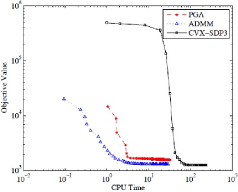
Figure 1: Comparison of ADMM, PGA, and CVX with SDP3 solver. ADMM converges faster.

3.3 Choice of the regularization parameters

The proposed convex minimization algorithm is fast and scalable, but it requires to set a relatively large number of regularization parameters. As with many structured sparsity formulations, a grid search on the held-out dataset performance is not practical and time-consuming. To speed up the adjustment of the regularization parameters, we used Gradient Free Optimization (GFO) , which minimizes the prediction loss on a held-out fraction of the training set. GFO requires only to compute the objective function, but it does not require gradient information. The objective function of GFO is a black-box that takes as input the regularization parameters to optimize. A review of algorithms and comparison of software implementations for a variety of GFO approaches is provided in Rios and Sahinidis (2012).

4 Experiments

We evaluate the performance of JLR, JL0, J0R, I0R, and J00 on synthetic data for matrix completion and on real-world data for image denoising and multi-label classification. In the following, we first explain the parameter tuning and evaluation criteria used in the experiments, and then discuss the results.

We used 5-fold cross-validation to obtain the optimum values for the regularization parameters. However, to simplify the optimization, we consider a slightly different formulation of the models. For example for JLR, we optimize w.r.t. $\lambda$ and $c$ where $0<c<1$ instead $\lambda_{0}$, $\lambda_{1}$ and $\lambda_{2}$. The resulting objective function is of the form $\lambda\left(\frac{1}{1-c}\|X_{0}\|_{*}+\frac{1}{c}\|X_{1}\|_{*}+\frac{1}{c}\|X_{2}\|_{*}\right)$. For $\lambda$, $\alpha_{1}$ and $\alpha_{2}$, we consider a range of $\{10^{-2},10^{-1},10^{0},10^{1},10^{2}\}$ and for $c$ we consider $c=\{0.1,0.2,\ldots,0.9\}$.

To evaluate the performance on the matrix completion problem, we use normalized prediction test error (which we call test error). We use one part of the data to train the models and test on the remaining part. For multi-label classification experiment, we use the same criteria as Goldberg et al. (2010), that is, the transductive label error. It corresponds to the percentage of incorrectly predicted labels and the relative feature reconstruction error.

4.1 Comparison of the solvers

As a sanity check, we compared our ADMM algorithm for JLR to off-the-shelf SDP solvers (using CVX with SDP3). We also implemented an alternative method based on the accelerated proximal gradient (PGA) Toh and Yun (2010) and we compared to it (see the appendix for a detailed description of PGA). We report the CPU runtime and the objective. We consider synthetically generated data with $n=100$. We compute the CPU time using the built-in function in MATLAB cputime. All algorithms run on a standard desktop computer with $2.5$ GHz CPU (dual core) and $4$ GB of memory. Figure 1 shows the results. It can be observed that ADMM is converging faster to the optimum value (the one found by CVX with duality gap $<10^{-8}$) than CVX and PGA. This illustrates the fact that, under general conditions when $\{\mu_{k}\}$ is an increasing unbounded sequence, and the objective function and constraints are both differentiable, ADMM converges to the optimum solution super Q-linearly like the Augmented Lagrangian Method Bertsekas (1982). An additional advantage of ADMM is that the optimal step size is just the penalty term $\mu_{k}$ which makes the algorithm free of tuning parameters, unlike iterative thresholding algorithms; PGA and other thresholding algorithms are only sub-linear in theory Lin et al. (2009).

4.2 Synthetic data experiments

We compare the prediction capabilities of JLR, JL0, J0R, J00, and I00 on synthetic datasets. We use randomly generated square matrices of size $n$ for our experiment. We generate matrices $X_{0}$, $X_{1}$, and $X_{2}$ with different rank ($r_{0}$, $r_{1}$, and $r_{2}$) as a product of $UV^{T}$ where $U$ and $V$ are generated randomly with Gaussian distribution and unitary noise. The noise matrices $E_{1}$ and $E_{2}$ are generated randomly with Gaussian distribution and unitary noise. The sparse matrices $S_{1}$ and $S_{2}$ are generated by choosing a sparse support set of size $k=0.1*n^{2}$ uniformly at random, and whose non-zero entries are generated uniformly in $[-a,a]$. For each setting, we repeat $10$ trials and report the mean and the standard deviation of the test error.

	test error	training loss	CPU time
JLR	$83.61\pm 4.19$	$79.29\pm 2.08$	$172.24\pm 1.92$
JL0	$89.52\pm 3.97$	$81.59\pm 2.14$	$149.14\pm 1.19$
J0R	$94.51\pm 4.02$	$85.37\pm 2.49$	$89.54\pm 2.01$
J00	$138.31\pm 3.92$	$92.47\pm 2.84$	$45.34\pm 1.21$
I0R	$131.43\pm 3.16$	$86.37\pm 2.59$	$41.26\pm 1.32$
I00	$142.57\pm 3.25$	$98.61\pm 3.31$	$46.82\pm 1.52$

Table 1: Performance on the synthetic datasets where $n=2000$, $d_{1}=d_{2}=1000$.

	test error	training loss	CPU time
JLR	$53.23\pm 2.25$	$27.43\pm 0.12$	$3.96\pm 0.19$
JL0	$59.45\pm 2.74$	$28.73\pm 0.15$	$2.71\pm 0.14$
J0R	$63.56\pm 2.17$	$29.76\pm 0.22$	$1.08\pm 0.21$
J00	$72.39\pm 2.32$	$45.37\pm 0.31$	$1.03\pm 0.29$
I0R	$69.25\pm 2.13$	$41.52\pm 0.23$	$1.02\pm 0.36$
I00	$76.41\pm 2.57$	$48.36\pm 0.27$	$1.01\pm 0.31$

Table 2: Performance on the synthetic datasets where $n=200$, $d_{1}=d_{2}=100$.

Tables 1 and 2 show the comparison of the approaches discussed in Section 2 for two different settings. Each cell shows the mean and standard deviation of the test error over $10$ simulations. The test prediction performances of JLR is superior compared to the other approaches. We also see that the training loss is lower in JLR approach. Note that the stopping criteria is a fixed number of iterations, and more complex take more time than simpler ones, but the loss of speed is only by a constant amout (JLR is about 3 times slower to learn than I00).

4.3 Image denoising

We evaluate the performance of JLR for image denoising and compare it against J0R and I0R. The image denoising is based on the Extended Yale Face Database B available at cvc.yale.edu/projects/yalefacesB.html. It contains image faces from 28 individuals under 9 different poses and 64 different lighting conditions. We choose two different lighting conditions (+000E+00 and +000E+20) as two views of an image. The intuition is that each view has low rank latent structure (due to the view-specific lightning condition), while each image share the same global structure (the same person with the same pose). Each image is down-sampled to $100\times 100$. So the dimension of the datasets based on our notation is: $d_{1}=10000$, and $d_{2}=10000$. We add $5\%$ noise to the randomly selected pixels of view 1 and view 2 as well as 40% of missing entries in both views. The goal is to reconstruct the image by filling in missing entries as well as removing the noise.

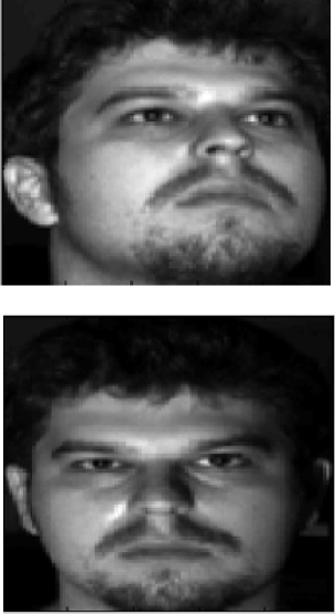
(a) Original

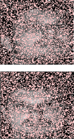
(b) Corrupted

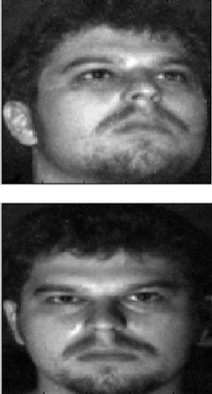
(c) JLR

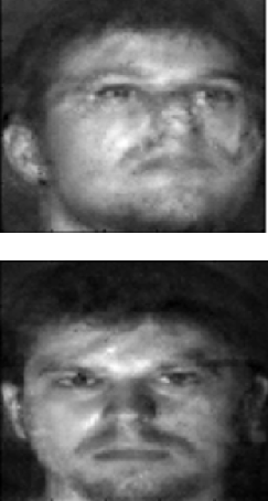
(d) J0R

(e) I0R

Figure 2: Reconstruction of a noisy image with $5\%$ uniform noise and $40\%$ missing entries at random. The reconstruction of noisy images by JLR is qualitatively better than the reconstruction by the other approaches. This is confirmed quantitatively in Table 3.

JLR	JL0	J0R	J00	I0R	I00
$0.0619$	$0.0621$	$0.0631$	$0.1002$	$0.0825$	$0.1012$

Table 3: Average test error (squared error) over $5$ random train-test splits for the Yale Face Dataset. The standard deviation was less than $10^{-3}$ in all cases.

Figure 2 shows the visualization performance in reconstructing the noisy image. J0R is successful in removing the noise but the quality of the reconstruction is visually worse than the JLR models that captures well the specific low-rank variations of each image. We also compare the test errors (squared loss) of the different models in Table 3. The visual intuition is confirmed by the fact that the best performances are obtained by JLR and JL0. Quantitatively, JLR only slightly outperforms JL0, but there is an important visual qualitative improvement in Figure 2.

4.4 Multi-label classification

We evaluate the applicability of JLR with a logistic loss on the second view in the context of a multi-label prediction task and compare it with the approach proposed by Goldberg et al. (2010). In this application, View 1 represents the feature matrix and View 2 the label matrix. In many real situations, the feature matrix is partially observed. One simple solution is to first impute the missing data in the feature matrix and then further proceed with the multi-label classification task. Another way is to treat the feature matrix and the label matrix as two views of the same object, and treating the labels to predict as missing entries. We also compared these algorithms against the state-of-the-art approaches for multi-label classification. We use Robust PCA (using our ADMM algorithm) for data imputation in the feature matrix and then use two different approaches in multi-label classification proposed in Zhang and Zhou (2007) and linear SVM. We consider two different datasets, both of which were used by Goldberg et al. (2010), namely: Yeast Micro-array data and Music Emotion data available at the following url: mulan.sourceforge.net/datasets.html.

	Label error percentage
	$\pi=40\%$	$\pi=60\%$	$\pi=80\%$
J00 Goldberg et al. (2010)	$16.7(0.3)$	$13.0(0.2)$	$8.5(0.4)$
J00 (ADMM)	$16.8(0.4)$	$13.1(0.2)$	$8.4(0.3)$
J0R	$16.4(0.2)$	$12.9(0.1)$	$8.1(0.2)$
JL0	$16.8(0.2)$	$13.0(0.1)$	$8.4(0.3)$
JLR	16.4(0.2)	12.8(0.1)	8.1(0.2)
Imputation + Zhang and Zhou (2007)	$20.3(0.2)$	$19.5(0.1)$	$18.4(0.1)$
Imputation + SVM	$21.6(0.3)$	$20.5(0.1)$	$20.4(0.2)$
	Relative feature reconstruction error
	$\pi=40\%$	$\pi=60\%$	$\pi=80\%$
J00 Goldberg et al. (2010)	$0.86(0.02)$	$0.92(0.00)$	$0.74(0.02)$
J00 (ADMM)	$0.83(0.01)$	$0.89(0.01)$	$0.71(0.01)$
J0R	$0.81(0.01)$	$0.86(0.01)$	$0.69(0.01)$
JL0	$0.82(0.01)$	$0.85(0.01)$	$0.70(0.01)$
JLR	0.74(0.01)	0.82(0.01)	0.67(0.01)
Imputation + Zhang and Zhou (2007)	$0.80(0.00)$	$0.75(0.02)$	$0.74(0.01)$
Imputation + SVM	$0.80(0.00)$	$0.75(0.02)$	$0.74(0.01)$

Table 4: Label prediction error comparison for Yeast data, where the first J00 is proposed in Goldberg et al. (2010).

	Label error percentage
	$\pi=40\%$	$\pi=60\%$	$\pi=80\%$
J00 Goldberg et al. (2010)	$27.4(0.8)$	$23.7(1.6)$	$19.8(2.4)$
J00 (ADMM)	$28.0(0.01)$	$24.1(0.02)$	$21.2(0.01)$
J0R	$28.0(0.01)$	$24.1(0.02)$	$21.2(0.01)$
JL0	$27.8(0.02)$	$23.0(0.05)$	$20.7(0.06)$
JLR	$27.8(0.02)$	23.0(0.05)	$20.7(0.06)$
Imputation + Zhang and Zhou (2007)	25.6(1.0)	$23.5(0.9)$	19.5(1.1)
Imputation + SVM	$26.7(0.7)$	$25.7(1.1)$	$24.3(1.5)$
	Relative feature reconstruction error
	$\pi=40\%$	$\pi=60\%$	$\pi=80\%$
J00 Goldberg et al. (2010)	$0.60(0.05)$	$0.46(0.12)$	$0.25(0.03)$
J00 (ADMM)	$0.58(0.01)$	$0.33(0.02)$	$0.12(0.01)$
J0R	$0.58(0.01)$	$0.33(0.02)$	$0.12(0.01)$
JL0	$0.56(0.02)$	$0.30(0.01)$	$0.10(0.01)$
JLR	$0.56(0.02)$	0.30(0.01)	0.10(0.01)
Imputation + Zhang and Zhou (2007)	0.47(0.01)	$0.31(0.02)$	$0.12(0.01)$
Imputation + SVM	$0.47(0.01)$	$0.31(0.02)$	$0.12(0.01)$

Table 5: Label prediction error comparison for music data, where the first J00 is copied from Goldberg et al. (2010).

The Yeast dataset contains $n=2417$ samples in $d_{1}=103$ dimensional space. Each sample can belong to one of $d_{2}=14$ gene functional classes and the goal is to classify each gene based on its function. We vary the percentage of observed value ($\pi=40\%$, $\pi=60\%$, and $\pi=80\%$). For each $\pi$, we run $10$ repetitions and report mean and standard deviation (in parenthesis). Parameters are tuned by cross validation on optimizing the label error prediction. The left columns of Table 4 show the label prediction error on Yeast dataset. We observe that J00 Goldberg et al. (2010) and J00 (ADMM) produce very similar results. We obtain a slightly lower label prediction error for J0R and JLR. The right columns in Table 4 show the relative feature reconstruction error. JLR outperforms other algorithms in relative feature reconstruction error. This is due to the fact that JLR is a richer model, better able to capture the underlying structure of the data. We compared these algorithms against a baseline in which $100\%$ of features are given (i.e., no missing entries) and predict the missing labels using SVM. The prediction performance for the baseline with $\pi=40\%,60\%,80\%$ is $20.9(0.1),19.4(0.3),18.8(0.2)$, respectively. A paired $t$-test shows that JLR outperforms the baseline at a significance level of $5\%$.

The Music dataset consists of $n=593$ songs in $d_{1}=72$ dimension (i.e., $8$ rhythmic and $64$ timbre-based) each one labeled with one or more of $d_{2}=6$ emotions (i.e., amazed-surprised, happy-pleased, relaxing-calm, quiet-still, sad-lonely, and angry-fearful). Features are automatically extracted from a 30-second sound clip. The left columns of Table 5 show the label prediction error. Similar to Yeast, we observe that J00 Goldberg et al. (2010) and J00 (ADMM) have the same label error performance. In this dataset, we see that JLR and JL0 produce the same results which suggests that the low-rank structure defined on the label matrix is sufficient to improve the prediction performance. The last columns of Table 5 show the relative feature reconstruction error. First, it should be noted that J00 (ADMM) has better results in relative feature reconstruction error compared to J00 Goldberg et al. (2010). This suggest the efficiency of ADMM implemented for J00. Moreover, we observe that JLR outperforms other algorithms in terms of relative feature reconstruction error. Again, we compared these algorithms against a baseline in which $100\%$ of features are given (i.e., no missing entries) and predict the missing labels using SVM. The prediction performance for the baseline with $\pi=40\%,60\%,80\%$ is $25.8(0.4),24.6(1.2),24.5(1.3)$, respectively. Using a paired $t$-test, JLR is statistically outperforming the baseline at the level of $5\%$ significance with $\pi=40\%,60\%$.

4.5 Optimization of regularization parameters

We checked wether grid search described at the beginning of this section is the best solution to optimize the cross-validation error with respect to the choice of the regularization parameters. After running experiments on synthetic data, we found that Stable Noisy Optimization using Branch and Fit (SNOBFIT) Huyer and Neumaier (2008) is one of the best algorithms among others for optimizing a black-box function both in terms of accuracy and time efficiency (i.e., compare to multilevel coordinate search (MCS) Huyer and Neumaier (1999) and simplex derivative pattern search method (SID-PSM) Custodio and Vicente (2008)). SNOBFIT is a Matlab package designed for selecting continuous parameter setting for simulations or experiments. It is based on global and local search by branching and local fit. We used freely available software for SNOBFIT (available at the following url: mat.univie.ac.at/~neum/software/snobfit/). We run experiment for Music emotion dataset and compare the results obtained by both SNOBFIT and grid search. Table 6 shows the predictive performances of the method after tuning the regularization parameters for JLR algorithm. The results show better predictive performances for both label prediction error and reconstruction error using SNOBFIT, but the speed was comparable between the two approaches.

	Label error percentage			Relative feature reconstruction error
	$\pi=40\%$	$\pi=60\%$	$\pi=80\%$	$\pi=40\%$	$\pi=60\%$	$\pi=80\%$
JLR-SNOBFIT	$25.9(0.04)$	$22.1(0.02)$	$19.3(0.03)$	$0.53(0.04)$	$0.29(0.03)$	$0.10(0.03)$
JLR-GRID	$27.8(0.02)$	$23.0(0.05)$	$20.7(0.06)$	$0.56(0.02)$	$0.30(0.01)$	$0.10(0.01)$

Table 6: Label prediction error comparison of SNOBFIT vs. grid search on the optimization of cross-validation error for music data.

5 Conclusion

We introduced a convex reformulation of inter-battery factor analysis, a method closely related to canonical correlation analysis. The proposed formulation enables us to easily handle missing data, to monitor the convergence of the estimation algorithm, and to develop scalable algorithms by exploiting tools from convex optimization. A natural extension of our work would be to develop stochastic algorithms to scale to even bigger datasets. On the modeling side, our approach would benefit from theoretical rank-recovery results to identify view-specific and shared latent subspaces. Experimentally, we showed that accounting for view-specific variations can significantly boost performance and that robust approaches are beneficial in practice. For tuning the regularizaiton parameter in our problem, we use gradient free optimization and show the accuracy can be improved. Future work include the use of overlapping trace norms for a broader class of problems, including collective matrix factorization and tensor factorization. We are also investigating smarter ways of selecting regularization parameters using generalization bounds or Bayesian approaches.

References

- Amini et al. (2010) M. R. Amini, N. Usunier, and C. Goutte. Learning from multiple partially observed views-an application to multilingual text categorization. In NIPS, 2010.
- Archambeau and Bach (2008) C. Archambeau and F. Bach. Sparse probabilistic projections. In NIPS, 2008.
- Archambeau et al. (2006) C. Archambeau, N. Delannay, and M. Verleysen. Robust probabilistic projections. In ICML, 2006.
- Bach and Jordan (2002) F. Bach and M. I. Jordan. Kernel independent component analysis. Journal of Machine Learning Research, 3:1–48, 2002.
- Bach and Jordan (2005) F. Bach and M. I. Jordan. A probabilistic interpretation of canonical correlation analysis. Technical Report 688, Department of Statistics, University of California at Berkeley, 2005.
- Bertsekas (1982) D. P. Bertsekas. Constrained optimization and lagrange multiplier methods. Computer Science and Applied Mathematics, Boston: Academic Press, 1982, 1, 1982.
- Borga (1998) M. Borga. Learning Multidimensional Signal Processing. PhD thesis, Linköping University, Sweden, 1998.
- Boyd et al. (2011) S. Boyd, N. Parikh, E. Chu, B. Peleato, and J. Eckstein. Distributed optimization and statistical learning via the alternating direction method of multipliers. Foundations and Trends® in Machine Learning, 3(1):1–122, 2011.
- Cabral et al. (2011) R. Cabral, F. De la Torre, J. Costeira, and A. Bernardino. Matrix completion for multi-label image classification. In NIPS, 2011.
- Cai et al. (2010) J. Cai, E. J. Candès, and Z. Shen. A singular value thresholding algorithm for matrix completion. SIAM Journal on Optimization, 20(4):1956–1982, 2010.
- Candès and Recht (2009) E. J. Candès and B. Recht. Exact matrix completion via convex optimization. Foundations of Computational Mathematics, 9(6):717–772, 2009.
- Candès et al. (2011) E. J. Candès, X. Li, Y. Ma, and J. Wright. Robust principal component analysis? Journal of the ACM, 58(3), 2011.
- Cannon and Hsieh (2008) A. J. Cannon and W. W. Hsieh. Robust nonlinear canonical correlation analysis: Application to seasonal climate forecasting. Nonlinear Processes in Geophysics, 15:221–232, 2008.
- Christoudias et al. (2012) C. Christoudias, R. Urtasun, and T. Darrell. Multi-view learning in the presence of view disagreement. arXiv preprint arXiv:1206.3242, 2012.
- Custodio and Vicente (2008) A. L. Custodio and L. Vicente. Sid-psm: A pattern search method guided by simplex derivatives for use in derivative-free optimization. Technical report, Departamento de Matemática, Universidade de Coimbra, Coimbra, 2008.
- Goldberg et al. (2010) A. B. Goldberg, X. Zhu, B. Recht, J.M. Xu, and R. Nowak. Transduction with matrix completion: Three birds with one stone. In NIPS, 2010.
- Hardoon et al. (2004) D. R. Hardoon, S. Szedmak, and J. Shawe-Taylor. Canonical correlation analysis: An overview with application to learning methods. Neural Computation, 16(12):2639–2664, 2004.
- Hotelling (1936) H. Hotelling. Relations between two sets of variates. Biometrika, 28(3/4):321–377, 1936.
- Huyer and Neumaier (1999) W. Huyer and A. Neumaier. Global optimization by multilevel coordinate search. Journal of Global Optimization, 14(4):331–355, 1999.
- Huyer and Neumaier (2008) W. Huyer and A. Neumaier. Snobfit–stable noisy optimization by branch and fit. ACM Transactions on Mathematical Software (TOMS), 35(2):9, 2008.
- Jia et al. (2010) Y. Jia, M. Salzmann, and T. Darrell. Factorized latent spaces with structured sparsity. In NIPS, 2010.
- Jolliffe (1986) I. T. Jolliffe. Principal Component Analysis. Springer-Verlag, New York, 1986.
- Klami et al. (2013) A. Klami, S. Virtanen, and S. Kask. Bayesian canonical correlation analysis. Journal of Machine Learning Research, 14:965–1003, 2013.
- Lin et al. (2009) Zh. Lin, M. Chen, and Y. Ma. The augmented lagrange multiplier method for exact recovery of corrupted low-rank matrices. Technical report, UIUC, 2009.
- MacKay (1996) D. J. C. MacKay. Bayesian methods for backpropagation networks. Models of Neural Networks III, 6:211–254, 1996.
- Parkhomenko et al. (2009) E. Parkhomenko, D. Tritchler, and J. Beyene. Sparse canonical correlation analysis with application to genomic data integration. Statistical Applications in Genetics and Molecular Biology, 8(1):1–34, 2009.
- Rios and Sahinidis (2012) L. M. Rios and V. N. Sahinidis. Derivative-free optimization: A review of algorithms and comparison of software implementations. Journal of Global Optimization, pages 1–47, 2012.
- Sturm (1999) J. F. Sturm. Using sedumi 1.02, a matlab toolbox for optimization over symmetric cones. Optimization methods and software, 11(1-4):625–653, 1999.
- Toh and Yun (2010) K. Toh and S. Yun. An accelerated proximal gradient algorithm for nuclear norm regularized linear least squares problems. Pacific Journal of Optimization, 6(615-640):15, 2010.
- Tucker (1958) L. R. Tucker. An inter-battery method of factor analysis. Psychometrika, 23(2):111–136, 1958.
- Virtanen et al. (2011) S. Virtanen, A. Klami, and S Kaski. Bayesian CCA via group sparsity. In ICML, 2011.
- White et al. (2012) M. White, Y. Yu, X. Zhang, and D. Schuurmans. Convex mult-view subspace learning. In NIPS, 2012.
- Zhang and Zhou (2007) M. Zhang and Z. Zhou. Ml-knn: A lazy learning approach to multi-label learning. Pattern Recognition, 40(7):2038–2048, 2007.