Kovacs-like memory effect in driven granular gases

Abstract

While memory effects have been reported for dense enough disordered systems such as glasses, we show here by a combination of analytical and simulation techniques that they are also intrinsic to the dynamics of dilute granular gases. By means of a certain driving protocol, we prepare the gas in a state where the granular temperature $T$ coincides with its long time limit. However, $T$ does not subsequently remain constant, but exhibits a non-monotonic evolution before reaching its non-equilibrium steady value. The corresponding so-called Kovacs hump displays a normal behavior for weak dissipation (as observed in molecular systems), but is reversed under strong dissipation, where it thus becomes anomalous.

At equilibrium, the response of a system to an external sudden perturbation, like a temperature jump, depends only on the macroscopic variables characterizing the state under study. On the other hand, in non-equilibrium situations, the observed response depends not only on the instantaneous value of the macroscopic variables, but also on the previous history. Memory effects are consequently ubiquitous out of equilibrium. A classic experiment in this context bears the name of Kovacs Ko63 ; Ko79 . A polymer sample, initially at equilibrium at a high temperature $T_{0}$, is rapidly quenched to a low temperature $T_{1}$, at which it evolves for a given waiting time $t_{w}$. Afterwards, the bath temperature is suddenly increased to $T$, with $T_{0}>T>T_{1}$, such that the instantaneous polymer volume $V$ equals its equilibrium value at $T$. The sample volume then does not remain constant for $t>t_{w}$: it first increases, displays a maximum, and returns to equilibrium for longer times only. This simple experiment shows that the macroscopic variables $(P,V,T)$ (the pressure $P$ being kept constant throughout the whole procedure) do not completely characterize the macroscopic state of the system: its response depends also on the previous thermal history.

This kind of crossover, or Kovacs memory effect, has been extensively investigated in glassy and other complex systems, starting from the phenomenological theory presented by Kovacs himself Ko79 . It is displayed by polymers, structural and spin glasses, compacting dense granular media, kinetically constrained models, classical and quantum spin models, distributions of two-level systems, etc. Ko63 ; Ko79 ; Br78 ; ByB02 ; ByH02 ; Bu03 ; BBDG03 ; CLyL04 ; AyS04 ; MyS04 ; TyV04 ; ALyN06 ; AAyN08 ; PyB10 ; ByL10 ; DyH11 ; RyP14 . The quantity displaying the hump may be different from the volume: in several of the previous studies, the energy is the relevant quantity. Interestingly, most of the observed behavior can be understood within a linear response theory approach, although the temperature jumps are usually not small in the experiments PyB10 ; DyH11 ; RyP14 .

Whereas the Kovacs effect has previously been reported for dense media, or systems exhibiting complex energy landscape, we focus here on a low density granular gas PyB03 ; ByP04 where the effect is a priori less expected. Due to inelastic collisions, a gas of grains is an intrinsically out-of-equilibrium system, arguably one of the simplest. Without external driving, its granular temperature – a measure of velocity fluctuations – monotonically decreases, and the granular gas may end up in the homogeneous cooling state (HCS), provided a small enough system is considered to prevent the development of long-wavelength instabilities GyS95 ; BRyC96 ; NyE98 . In order to reach a non-equilibrium steady state, one needs a mechanism that inputs energy into the set-up. With the stochastic thermostat NyE98 ; ENTyP99 , additional white noise forces act over each grain independently. This simple forcing mechanism is relevant for some two-dimensional experimental configurations with a rough vibrating piston PEyU02 , and also appears as a limiting case of a granular system heated by elastic collisions Sa03 . Although these thermostatted or heated granular fluids have been extensively investigated WM96 ; NyE98 ; ENTyP99 ; MyS00 ; SyM09 ; MGyT09 ; ETB06 ; Z09 ; GMyT12 ; GMyT13 ; P98 ; CVyG13 , no attention has been paid to memory effects. On the other hand, in compaction processes of dense granular systems, the relevance of history has been assessed, both experimentally and theoretically: Its evolution under a given driving depends not only on the instantaneous value of its packing fraction, but also on the previous driving protocol TyV04 ; JTMyJ00 ; He00 ; ByP01 ; ByL01 ; ByP02 ; RDRNyB05 ; RRPByD07 .

A valid question in granular gases is the type and number of variables that completely characterize a macroscopic state rque20 . In the non-driven case, the HCS is the reference state for developing the hydrodynamics, and it suffices to give the granular temperature. The same holds for the Gaussian thermostatted case MyS00 ; Lu01 ; BRyM04 , which can be mapped onto the HCS. On the other hand, there is some evidence that additional variables are necessary for other drivings like the stochastic thermostat. This uniformly heated granular gas evolves to a hydrodynamic solution of the Boltzmann equation GMyT12 ; GMyT13 , the so-called $\beta$-state where $\beta$ is a parameter that keeps track of the distance to stationarity (see below). Therein, the granular temperature is a monotonic function of time and, together with the driving intensity, completely characterizes the $\beta$-state. One may thus naively conclude that no Kovacs hump should be expected. We show below that such a surmise is incorrect: not only is the Kovacs effect present, but it also changes sign depending on dissipation. An anomalous Kovacs effect is thereby brought to bear for strongly dissipative systems.

In short, our motivation is two-fold. First, adapting the celebrated Kovacs protocol, we wish to study if memory can be encoded in a seemingly plain system with a trivial energy landscape, which is all kinetic. Second, the goal is to illustrate for the fact that, for a given driving amplitude, a single index (temperature) is insufficient to describe the non-equilibrium behavior of our homogeneous gas. One must keep track also of the non-Gaussianities of the velocity fluctuations, through the excess kurtosis. It appears that these non-Gaussianities are necessary, although not sufficient in general, for the occurrence of the hump.

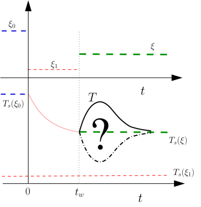
Figure 1: Top: Sketch of the drive time dependence. Bottom: Ensuing temperature evolution. At $t=0$, the gas is at temperature $T_{s}(\xi_{0})$, in the non-equilibrium steady state corresponding to a value of the driving $\xi_{0}$. At $t=0$, the drive is suddenly decreased to $\xi_{1}\ll\xi_{0}$, which is kept for a waiting time $t_{w}$. At $t=t_{w}$, the granular temperature is measured, and the driving is cranked up to a new value $\xi$, such that $T_{\text{s}}(\xi)=T(t_{w})$. The question mark is for the two possible scenarios: a positive hump with a $T$ maximum (normal behavior, solid line), or a negative anomalous hump (dot-dashed line). At long times, $T$ reaches its steady value $T_{s}(\xi)$.

The system at hand comprises $N$ inelastic smooth hard particles of mass $m$ and diameter $\sigma$. When particles $i$ and $j$ collide, momentum is conserved but kinetic energy is not. The inelasticity is characterized by the coefficient of normal restitution $\alpha$ (taken independent of the relative velocity): $\bm{\sigma}\cdot\bm{v}^{\prime}_{ij}=-\alpha\,\bm{\sigma}\cdot\bm{v}_{ij}$, in which $\bm{v}^{\prime}_{ij}$ is the post-collisional relative velocity, $\bm{v}_{ij}$ the pre-collisional one, and $\widehat{\bm{\sigma}}$ the unit vector joining the centers of particles $j$ and $i$. Moreover, grains are submitted to independent white noise forces, and we assume that the system remains spatially homogeneous, as backed up by molecular dynamics simulations ENTyP99 . Then, the velocity probability distribution is a sole function of velocity and time, and obeys NyE98 ; ENTyP99 ; Sa03 ,

$$\partial_{t}f(\bm{v}_{1},t)=\sigma^{d-1}\!\int d\bm{v}_{2}\int d\widehat{\bm{\sigma}}\,\Theta(\bm{v}_{12}\cdot\widehat{\bm{\sigma}})(\bm{v}_{12}\cdot\widehat{\bm{\sigma}})$$

$$\qquad\times(\alpha^{-2}b_{\sigma}^{-1}-1)f(\bm{v}_{1},t)f(\bm{v}_{2},t)+\frac{\xi^{2}}{2}\nabla^{2}_{\bm{v}_{1}}f(\bm{v}_{1},t)$$ (1)

In the Boltzmann-Fokker-Planck equation above, $\xi$ is the noise strength, $d$ is the dimension of space, $\Theta$ is Heaviside function, and the operator $b_{\sigma}^{-1}$ replaces the velocities $\bm{v}_{1}$ and $\bm{v}_{2}$ by the pre-collisional ones.

The granular temperature $T(t)$ is defined as the second moment of the distribution,

$$n\left\langle\frac{1}{2}mv^{2}(t)\right\rangle\equiv\int d\bm{v}\frac{1}{2}mv^{2}f(\bm{v},t)=\frac{d}{2}nT(t),$$ (2)

where $n=\int d\bm{v}f(\bm{v},t)$ is the particle density. In the theory developed here, a central role is played by the excess kurtosis $a_{2}$ of the velocity fluctuations,

$$a_{2}=\frac{d}{d+2}\frac{\langle v^{4}\rangle}{\langle v^{2}\rangle^{2}}-1,$$ (3)

which vanishes for a Gaussian distribution. The general $n$-th moment is given by $\langle v^{n}\rangle\equiv n^{-1}\int d\bm{v}\,v^{n}f(\bm{v},t)$. In the long time limit, the granular gas reaches a steady state in which the energy loss due to collisions is balanced on average by the energy input from the stochastic thermostat. The stationary values of the granular temperature $T_{\text{s}}$ and excess kurtosis $a_{2}^{\text{s}}$ are NyE98

$$T_{\text{s}}=\left[\frac{m\xi^{2}}{\zeta_{0}(1+\frac{3}{16}a_{2}^{\text{s}})}\right]^{2/3},\quad\zeta_{0}=\frac{2n\sigma^{d-1}\left(1-\alpha^{2}\right)\pi^{\frac{d-1}{2}}}{\sqrt{m}d\Gamma(d/2)},$$ (4a)

$$a_{2}^{\text{s}}=\frac{16(1-\alpha)(1-2\alpha^{2})}{73+56d-24d\alpha-105\alpha+30(1-\alpha)\alpha^{2}}.$$ (4b)

The main assumptions in deriving these steady values are (i) the first-Sonine approximation (ii) the smallness of non-linear terms in the excess kurtosis, which are thus neglected (see e.g. NyE98 ). For our purposes, it is convenient to introduce rescaled, order of unity variables,

$$\beta=\sqrt{\frac{T_{\text{s}}}{T}},\quad A_{2}=\frac{a_{2}}{a_{2}^{\text{s}}},\quad\uptau=\frac{\zeta_{0}\sqrt{T_{\text{s}}}}{2}t.$$ (5)

Starting from the Boltzmann-Fokker-Planck equation (1), one can derive the evolution equations for the granular temperature and the excess kurtosis NyE98 ; GMyT12 ; PyT13 ,

$$\frac{d\beta}{d\uptau}=1-\beta^{3}+\frac{3}{16}a_{2}^{\text{s}}\left(A_{2}-\beta^{3}\right),$$ (6a)

$$\beta\frac{dA_{2}}{d\uptau}=4\left[\left(1-\beta^{3}\right)A_{2}+B\left(1-A_{2}\right)\right],$$ (6b)

which are nonlinear in $\beta$ but linear in the excess kurtosis, consistently with our approach. Obviously, $\beta=1$ and $A_{2}=1$ is a stationary solution. The parameter $B$ is a given function of the restitution coefficient and of the dimension of space. We find it from a self-consistency argument: when the driving is so small that $\beta\to 0$, $a_{2}$ evolves to its value $a_{2}^{\text{HCS}}$ for the HCS SyM09 ,

$$a_{2}^{\text{HCS}}=\frac{16(1-\alpha)(1-2\alpha^{2})}{25+2\alpha(\alpha-1)+24d+\alpha(8d-57)}.$$ (7)

Thus, $A_{2}=a_{2}^{\text{HCS}}/a_{2}^{\text{s}}$ should be a root of the right hand side of Eq. (6b), and $B=a_{2}^{\text{HCS}}/(a_{2}^{\text{HCS}}-a_{2}^{\text{s}})$, that is,

$$B\,=\,\frac{73+8d(7-3\alpha)+15\alpha[2\alpha(1-\alpha)-7]}{16(1-\alpha)(3+2d+2\alpha^{2})}.$$ (8)

Let us address the Kovacs-like experiment depicted in Fig. 1. We would like to investigate the behavior of the granular temperature $T$ for $t>t_{w}$. If the pair $(\xi,T)$ does not completely characterize the state of the system, and other variables should be taken into account, $T$ will not remain constant but separate from its steady (initial) value and have either a maximum or a minimum. In molecular systems, there always appears a maximum in the Kovacs hump. This does not have to be the case for the granular temperature, because the granular gas is an intrinsically dissipative, out-of-equilibrium, system.

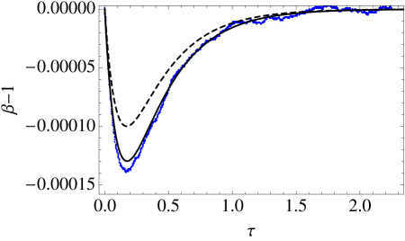
Figure 2: Plot of the Kovacs hump for $\alpha=0.3$ (top) and $\alpha=0.8$ (bottom). Monte Carlo simulation curves (points) for a system of $10^{4}$ hard disks ($d=2$), averaged over $10^{5}$ (top) and $1.5\times 10^{6}$ trajectories (bottom). They are compared to the theoretical curve (9b): the dashed line corresponds to the predicted values of $a_{2}^{\text{s}}$, $a_{2}^{\text{ini}}$ and $B$, while the solid line is obtained by taking these three parameters from the simulation (see e.g. Fig. 3, from which $B$ is directly measured). The sign of $\beta-1$ changes from the highly inelastic (top) to the weakly inelastic (bottom) case. Note that a maximum of $\beta$ corresponds to a minimum of $T=T_{\text{s}}/\beta^{2}$ (and vice versa), so that the Kovacs hump is anomalous in the highly inelastic region.

Defining the shifted time variable $\uptau=\zeta_{0}\sqrt{T_{s}}(t-t_{w})/2$, we have to solve Eqs. (6) with the initial conditions $\beta(\uptau=0)=1$ and $A_{2}(\uptau=0)=a_{2}^{\text{ini}}/a_{2}^{\text{s}}$, where $a_{2}^{\text{ini}}$ is the value of the excess kurtosis in the final state of the waiting time window. Since $a_{2}^{\text{s}}$ is small ($|a_{2}^{\text{s}}|\leq 0.07$) across the whole range of restitution coefficients, while $\beta$ and $A_{2}$ are of the order of unity, we expand both $\beta$ and $A_{2}$ in powers of $a_{2}^{\text{s}}$ to obtain an approximate solution of Eqs. (6)PyT13 ,

$$\quad a_{2}(\uptau)-a_{2}^{\text{s}}\,\sim\,(a_{2}^{\text{ini}}-a_{2}^{\text{s}})\,e^{-4B\uptau},$$ (9a)

$$\beta(\uptau)-1\,\sim\,\frac{3\left(a_{2}^{\text{ini}}-a_{2}^{\text{s}}\right)}{16(4B-3)}\left(e^{-3\uptau}-e^{-4B\uptau}\right).$$ (9b)

The relaxation of the excess kurtosis to its steady value is exponential, while that of the rescaled temperature $\beta$ is the sum of two exponentials with different relaxation times. The sign of $\beta-1$ is the same as that of $a_{2}^{\text{s}}$ because (i) $4B>3$ and (ii) $(a_{2}^{\text{ini}}-a_{2}^{\text{s}})$ and $a_{2}^{\text{s}}$ have the same sign as a function of the restitution coefficient for the arbitrary “cooling” ($\xi_{0}>\xi>\xi_{1}$) protocol in Fig. 1. In fact, Eq. (6b) predicts that $dA_{2}/d\uptau$ is initially positive and thus $|a_{2}|>|a_{2}^{\text{s}}|$ in the whole waiting time window PyT13 . In addition, the steady excess kurtosis $a_{2}^{\text{s}}$ changes sign at $\alpha_{c}=1/\sqrt{2}\simeq 0.707$: $a_{2}^{\text{s}}>0$ for $\alpha<\alpha_{c}$ while $a_{2}^{\text{s}}<0$ for $\alpha>\alpha_{c}$ alpha_c . Thus, for small inelasticity ($\alpha>\alpha_{c}$), $\beta-1<0$ and $\beta$ has a minimum, while the granular temperature $T=T_{\text{s}}/\beta^{2}$ has a maximum. This behavior is completely similar to that of glassy systems, so we may speak of a normal Kovacs hump in the weakly dissipative case. On the contrary, for high inelasticity, $\alpha<\alpha_{c}$, $\beta-1>0$ and $\beta$ displays a maximum, which corresponds to a minimum of $T$: an anomalous Kovacs hump appears.

In Fig. 2, the above theoretical prediction for the Kovacs hump is tested against numerical computations. The latter are obtained by means of direct Monte Carlo simulations Bi94 of the Boltzmann-Fokker-Planck equation (1). Two values of the restitution coefficient are considered: (i) $\alpha=0.3<\alpha_{c}$ (top, high inelasticity), and (ii) $\alpha=0.8>\alpha_{c}$ (bottom, low inelasticity). For the sake of concreteness, we take the limiting case (i) $\xi_{1}=0$ (the granular gas freely cools in the time window $0<t<t_{w}$) and (ii) a long enough $t_{w}$, so that $a_{2}^{\text{ini}}=a_{2}^{\text{HCS}}$. This choice (i)-(ii) is somewhat immaterial for what follows, because the whole dependence of the Kovacs hump on $\xi_{1}$ and $t_{w}$ is encoded in the initial value of the excess kurtosis difference $a_{2}^{\text{ini}}-a_{2}^{\text{s}}$, which in turn only changes the scale of the hump but does not alter its shape rque50 . In both cases, the dashed line corresponds to the theoretical prediction, Eq. (9b), in which the values of $a_{2}^{\text{s}}$, $B$, and $a_{2}^{\text{HCS}}$ are given by Eqs. (4b), (7) and (8), respectively. The agreement is reasonable: in particular, the sign of the hump is correctly predicted, but there are quantitative discrepancies. The latter stem from errors (of up to $10\%$) in the theoretical estimates of $a_{2}$ and $B$ GMyT12 . The quantitative agreement can be improved by inserting into (9b) their simulation values PyT13 , which yields the solid line. In particular, $B$ is extracted from Fig. 3, which furthermore corroborates the prediction of Eq. (9a).

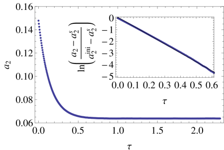
Figure 3: Decay of the excess kurtosis from its initial to its steady state value $a_{2}^{\text{s}}$. Plotted is the simulation curve obtained by the direct Monte Carlo scheme for $\alpha=0.3$. In the inset, the same decay but on a logarithmic scale. The linear slope is directly related to the parameter $B$, see (9a).

In order to understand the physical mechanism responsible for the observed behavior, a central idea is that the energy dissipation rate $d$ (“cooling rate” in the granular gas literature) increases with the excess kurtosis NyE98 . Moreover, the unforced system has stronger non-Gaussanities than the driven one, $|a_{2}^{\text{HCS}}|>|a_{2}^{\text{s}}|$ additional_friction , because the latter is randomized from stochastic ’kicks’ due to the forcing. For small inelasticities ($\alpha>\alpha_{c}$), $a_{2}^{\text{HCS}}$ and $a_{2}^{\text{s}}$ are both negative, so that $a_{2}^{\text{HCS}}<a_{2}^{\text{s}}$ and at $t=t_{w}$ the system has the steady value of the granular temperature but a dissipation rate smaller than that at stationarity $d_{\text{s}}$, $d/d_{\text{s}}<1$. Therefore, the granular temperature $T$ first increases and passes through a maximum ($\beta$ minimum) before returning to its steady value. For high inelasticities ($\alpha<\alpha_{c}$), $a_{2}^{\text{HCS}}$ and $a_{2}^{\text{s}}$ are both positive, so that $a_{2}^{\text{HCS}}>a_{2}^{\text{s}}$. Then, the system is at $t=t_{w}$ transiently in a state with $d/d_{\text{s}}>1$, so that $T$ initially decreases and passes through a minimum ($\beta$ maximum), see the table.

inelasticity	$\alpha$	$a_{2}^{\text{HCS}}-a_{2}^{\text{s}}$	$d/d_{\text{s}}$	$T$ hump (Kovacs)
“low”	$\;>\alpha_{c}\;$	$\;<0\;$	$\;<1\;$	maximum (normal)
“high”	$\;<\alpha_{c}\;$	$\;>0\;$	$\;>1\;$	minimum (anomalous)

Table 1: Summary of the Kovacs hump phenomenology and the underlying physical mechanism for the driving protocol in Fig. 1, with $\xi_{1}\ll\xi_{0}$.

The existence of the Kovacs hump, as given by Eq. (9b), is a crisp proof that the granular temperature does not suffice for characterizing the state of uniformly heated granular gases. Moreover, it links granular gases and other complex, non-equilibrium, systems. Nevertheless, this crossover effect is not a direct extension of the similar phenomenon observed in the latter: here we are dealing with an intrinsically out of equilibrium system relaxing to a far from equilibrium steady state. Furthermore, for the protocol considered, the intrinsically dissipative dynamics makes the Kovacs hump anomalous for high inelasticity. The hump is normal for the weakly dissipative case and disappears in the elastic limit $\alpha\to 1$, in which both $a_{2}^{\text{HCS}}$ and $a_{2}^{\text{s}}$ vanish. If we considered a “heating” protocol, that is, $\xi_{0}<\xi<\xi_{1}$, Eq. (6b) would give that $dA_{2}/d\uptau$ is initially negative: $|a_{2}|<|a_{2}^{\text{s}}|$ in the waiting time window. Then, $a_{2}^{\text{ini}}-a_{2}^{\text{s}}$ would have the sign opposite to that of $a_{2}^{\text{s}}$ and the sign of the hump would be reversed as compared to the behavior shown in the table. Here again, the normal behavior appears for low inelasticity, since in molecular systems, the energy displays a minimum for such “heating” protocols DyH11 .

Provided that the first-Sonine approximation to the Boltzmann equation remains valid, some of our main results are expected to hold for almost any uniformly heated granular gas: (i) the proportionality of the hump to the difference of excess kurtosis $(a_{2}^{\text{ini}}-a_{2}^{\text{s}})$, (ii) the exponential relaxation of the excess kurtosis, (iii) the two-exponential structure of the granular temperature relaxation. A singular case would be that of the Gaussian-thermostatted system, which can be mapped onto the HCS: In particular, its excess kurtosis equals $a_{2}^{\text{HCS}}$ and no hump would be observed. This is consistent, since the granular temperature completely specifies the HCS. Moreover, this clearly shows that the generic non-Maxwellian ($a_{2}\neq 0$) character of the velocity distribution function of granular gases is not a sufficient condition for the existence of the crossover effect.

The formalism developed here is thus quite general and may open the door to further general results in non-equilibrium statistical physics. In particular, the anomalous Kovacs hump for high inelasticity deserves further investigation. Linear response results PyB10 ; DyH11 ; RyP14 , closely related to the fluctuation-dissipation theorem, assure that the Kovacs hump is normal in molecular systems. In this regard, it would be interesting to analyze the possible connection between this anomaly and the validity of fluctuation-dissipation-like relations in dissipative systems PByL02 ; PByV07 ; MGyT09 ; PLyH11-12 ; BMyG12 .

- (1) A. J. Kovacs, Adv. Polym. Sci. (Fortschr. Hochpolym. Forsch.) 3, 394 (1963).
- (2) A. J. Kovacs, J. J. Aklonis, J. M. Hutchinson, and A. R. Ramos, J. Pol. Sci. 17, 1097 (1979).
- (3) S. A. Brawer, Phys. Chem. Glasses 19, 48 (1978).
- (4) L. Berthier and J. P. Bouchaud, Phys. Rev. B 66, 054404 (2002).
- (5) L. Berthier and P. C. W. Holdsworth, Europhys. Lett. 58, 35 (2002).
- (6) A. Buhot, J. Phys. A: Math. Gen. 36, L12367 (2003).
- (7) E. M. Bertin, J.-P. Bouchaud, J.-M. Drouffe, C. Godrèche, J. Phys. A: Math. Gen. 36, 10701 (2003).
- (8) L. F. Cugliandolo, G. Lozano, and H. Lozza, Eur. Phys. J. B 41, 87 (2004).
- (9) J. J. Arenzon and M. Sellitto, Eur. Phys. J. B 42, 543 (2004).
- (10) S. Mossa S and F. Sciortino, Phys. Rev. Lett. 92, 045504 (2004).
- (11) G. Tarjus and P. Viot, in Unifying Concepts in Granular Media and Glasses, A. Coniglio, A. Fierro, and M. Nicodemi eds. (Elsevier, Amsterdam, 2004) pp 35-45.
- (12) G. Aquino, L. Leuzzi, and T. M. Nieuwenhuizen, Phys. Rev. B 73, 094205 (2006).
- (13) G. Aquino, A. Allahverdyan, and T. M. Nieuwenhuizen, Phys. Rev. Lett. 101, 015901 (2008).
- (14) A. Prados and J. J. Brey, J. Stat. Mech.: Theor. Exp. P02009 (2010).
- (15) E. Bouchbinder and J. S. Langer, Soft Matter 6, 3065 (2010).
- (16) G. Diezemann and A. Heuer, Phys. Rev. E 83, 031505 (2011).
- (17) M. Ruiz-García and A. Prados, Phys. Rev. E 89, 012140 (2014).
- (18) T. Pöschel and N. Brilliantov eds., Granular Gas Dynamics, (Springer, Berlin, 2003).
- (19) N. Brilliantov and T. Pöschel, Kinetic Theory of Granular Gases (Clarendon Press, Oxford, 2004).
- (20) A. Goldshtein and M. Shapiro, J. Fluid. Mech. 282, 75 (1995).
- (21) J. J. Brey, M. J. Ruiz-Montero, and D. Cubero, Phys. Rev. E 54, 3664 (1996).
- (22) T. P. C. van Noije, and M. H. Ernst, Granular Matter 1, 57 (1998).
- (23) T. P. C. van Noije, M. H. Ernst, E. Trizac, and I. Pagonabarraga, Phys. Rev. E 59, 4326 (1999).
- (24) A. Prevost, D.A. Egolf, and J.S. Urbach, Phys. Rev. Lett. 89, 084301 (2002).
- (25) A. Santos, Phys. Rev. E 67, 051101 (2003).
- (26) D. R. M. Williams and F. C. MacKintosh, Phys. Rev. E 54, R9 (1996).
- (27) J. M. Montanero and A. Santos, Granular Matter 2, 53 (2000).
- (28) A. Santos and J. M. Montanero, Granular Matter 11, 157 (2009).
- (29) P. Maynar, M. I García de Soria, and E. Trizac, Eur. Phys. J. Special Topics 179, 123 (2009).
- (30) M. H. Ernst, E. Trizac, and A. Barrat, J. Stat. Phys. 124, 549 (2006).
- (31) K. Vollmayr-Lee, T. Aspelmeier, and A. Zippelius Phys. Rev. E 83, 011301 (2011).
- (32) M. I. García de Soria, P. Maynar, and E. Trizac, Phys. Rev. E 85, 051301 (2012).
- (33) M. I. García de Soria, P. Maynar, and E. Trizac, Phys. Rev. E 87, 022201 (2013).
- (34) A slight variant of the model can be found in A. Puglisi, V. Loreto, U. M. B. Marconi, and A. Vulpiani, Phys. Rev. E 59, 5582 (1999). See also CVyG13 .
- (35) M. G. Chamorro, F. Vega-Reyes, and V. Garzó, J. Stat. Mech. (Theor. Exp.) P07013 (2013).
- (36) C. Josserand, A. V. Tkachenko, D. M. Mueth, and H. M. Jaeger, Phys. Rev. Lett. 85, 3632 (2000).
- (37) D. A. Head, Phys. Rev. E 62, 2439 (2000).
- (38) J. J. Brey and A. Prados, Phys. Rev. E 63, 061301 (2001).
- (39) A. Barrat and V. Loreto, Europhys. Lett. 53, 297 (2001).
- (40) J. J. Brey and A. Prados, J. Phys: Cond. Matt. 14, 1489 (2002).
- (41) P. Richard, M. Nicodemi, R. Delannay, P. Ribière, and D. Bideau, Nature Materials 4, 121 (2005).
- (42) Ph. Ribière, P. Richard, P. Philippe, D. Bideau, and R. Delannay, Eur. Phys. J. E 22, 249 (2007).
- (43) Note that we will address here homogeneous configurations, without macroscopic flow.
- (44) J. Lutsko, Phys. Rev. E 63, 061211 (2001).
- (45) J. J. Brey, M. J. Ruiz-Montero, and F. Moreno, Phys. Rev. E 69, 051303 (2004).
- (46) A. Prados and E. Trizac, to be published.
- (47) The accuracy of this theoretical value of has been checked numerically, see for instance MyS00 .
- (48) G. Bird, Molecular Dynamics and the Direct Simulation of Gas Flows (Clarendon, Oxford, 1994).
- (49) For a finite value of , there exists an optimal waiting time for which is maximal. For , the optimal waiting time corresponds to PyT13 .
- (50) The same property holds when an additional friction force, coming from the thermal bath, is taken into account CVyG13 . Thus, the qualitative behavior discussed below is expected to remain valid for that case.
- (51) A. Puglisi, A. Baldassarri, and V. Loreto, Phys. Rev. E 66, 061305 (2002).
- (52) A. Puglisi, A. Baldassarri, and A. Vulpiani, J. Stat. Mech: Theor. Exp. P08016 (2007).
- (53) A. Prados, A. Lasanta, and P. I. Hurtado, Phys. Rev. Lett. 107, 140601 (2011); Phys. Rev. E 86, 031134 (2012).
- (54) J. J. Brey, P. Maynar, and M. I. García de Soria, Phys. Rev. E 86, 061308 (2012).