A Bayesian Method for the Intercalibration of Spectra in Reverberation Mapping

Abstract

Flux calibration of spectra in reverberation mapping (RM) is most often performed by assuming the flux constancy of some specified narrow emission lines, which stem from an extended region that is sometimes partially spatially resolved, in contrast to the point-like broad-line region and the central continuum source. The inhomogeneous aperture geometries used among different observation sets in a joint monitoring campaign introduce systematic deviations to the fluxes of broad lines and central continuum, and intercalibration over these data sets is required. As an improvement to the previous empirical correction performed by comparing the (nearly) contemporaneous observation points, we describe a feasible Bayesian method that obviates the need for (nearly) contemporaneous observations, naturally incorporates physical models of flux variations, and fully takes into account the measurement errors. In particular, it fits all the data sets simultaneously regardless of samplings and makes use of all of the information in the data sets. A Markov Chain Monte Carlo implementation is employed to recover the parameters and uncertainties for intercalibration. Application to the RM data sets of NGC 5548 with joint monitoring shows the high fidelity of our method.

1. Introduction

Reverberation mapping (RM) is a well-established technique for the study of broad-line regions (BLRs) in active galactic nuclei (AGNs) with broad emission lines (Blandford & McKee 1982; Peterson 1993). With appropriate analysis, RM experiments divulge the geometry, kinematic, and ionization structure information of BLRs (e.g., Brewer et al. 2011; Pancoast et al. 2012; Li et al. 2013). Over the past two decades, the BLR size derived using the time delay between the continuum variation and the broad emission line response has been utilized with great success to measure the mass of the central supermassive black hole by combining it with the width of the broad emission line (e.g., Peterson et al. 2004). The tight relationship between BLR sizes and optical luminosities of AGNs plays a key role in the demography of supermassive black holes in large AGN surveys (e.g., Bentz et al. 2013, and references therein).

At present there are $\sim$50 nearby Seyfert galaxies and quasars with RM measurements in the literature (e.g., Bentz et al. 2013), although a huge amount of effort has been invested in RM experiments. In practice, an RM campaign is quite observationally intensive and requires monitoring an object over a sufficient period with reasonable temporal resolution. Such high demand of time interval and sampling leads RM programs to be commonly undertaken by cooperative observations at multiple observatories, such as the well-known AGN Watch Project (Peterson et al. 2002) and MDM campaigns (Denney et al. 2010; Grier et al. 2012). Spectra calibration is most often based on the assumption that [O III] $\lambda$5007 line remains constant in flux over the timescale of interest and all spectra are scaled to an adopted absolute flux of [O III] $\lambda$5007, which can be measured on photometric nights (Peterson et al. 1991; van Groningen & Wanders 1992). The problem that arises with using [O III] $\lambda$5007 for such a calibration is that its emission region (narrow-line region; NLR) is sometimes spatially resolved and the size is most likely comparable with or even larger than the aperture size, in contrast to the effectively point-like BLR and central continuum sources. Consequently, the inhomogeneous aperture geometries used among different observation sets in a joint monitoring campaign admit different amounts of light from the NLR, and therefore introduce systematic deviations to the fluxes of broad emission lines (Peterson et al. 1995). Similarly, this effect also influences the central continuum fluxes contaminated by the host galaxy starlight.

Peterson et al. (1995) proposed an empirical correction to such an aperture effect by adopting one of the data set as standard, and applying a multiplicative scale factor and an additive flux adjustment to the other sets to bring the closely spaced measurements from the two sets into agreement. In reality, it is always impractical to base the correction on exactly contemporaneous observations. One has to relax such strict simultaneity and instead use pairs of observations that are closely separated (usually by more than one days), depending on the sampling of each data set. This apparently degrades the highest achievable temporal resolution.

In this Letter, we describe a novel method for intercalibration of reverberation mapping data that obviates the need for (nearly) contemporaneous observations, naturally incorporates physical models of flux variations, and fully takes into account the measurement errors. The method is based on Bayesian statistics and is sufficiently elastic to automated program manipulation.

2. Description of the Method

2.1. Variability Modeling

While variability across all bandpasses is one of the outstanding characteristics of AGNs (Ulrich et al. 1997), its underlying mechanisms remain inconclusive. There are recent extensive studies on the nature of AGN variability that are devoted to, but not limited to, exploring the ensemble properties of variability and its correlations with physical parameters of the AGN (e.g., Zuo et al. 2012; Ai et al. 2013; MacLeod et al. 2012; Meusinger & Weiss 2013); constructing the analytic stochastic description (e.g., Kelly et al. 2009, 2011; Kozłowski et al. 2010; MacLeod et al. 2010; Zu et al. 2013); and testing/applying physically motivated models for variability (e.g., Reynolds & Miller 2009; Dexter & Agol 2011; Pecháček et al. 2013 and references therein). Numerical simulations show that AGN variability is plausibly linked to some hydrodynamic or magnetohydrodynamic instabilities/turbulence within accretion disks, although such simulations are still in an early stage (e.g., Noble & Krolik 2009; Reynolds & Miller 2009). Using well sampled optical light curves of AGNs, it has been found that the optical power spectral density (PSD) of AGN variability can be described by a power law $P(f)\propto f^{-\alpha}$ with flattening to a constant below some break frequency that typically corresponds to a timescale of dozens of days (Czerny et al. 1999; Kelly et al. 2009, 2011; MacLeod et al. 2010). The slope $\alpha$ of the optical PSD seems to depend on the temporal frequency under consideration, changing from $\sim 2$ on a timescale of days (Kelly et al. 2009; Zu et al. 2013), the normal temporal resolution of ground-based RM campaigns, to steeper values on much a shorter timescale, which, however, is based on a very preliminary analysis of the Kepler data archive (Mushotzky et al. 2011). These features motivate the statistical modeling of variability of AGN optical continuum by a damped random walk (DRW) process with great success (Kelly et al. 2009, 2011). This is further reinforced by subsequent investigations of large samples of AGN light curves (Kozłowski et al. 2010; MacLeod et al. 2010; Zu et al. 2013; Li et al. 2013).

Specifically, a DRW process is a stationary process such that its covariance function at any two times $t_{1}$ and $t_{2}$ depends only on the time difference $t=|t_{1}-t_{2}|$ and has the form of

$$S(t)=\sigma^{2}\exp\left(-\frac{t}{\tau}\right),$$ (1)

where $\tau$ is the damping timescale of the process to return to its mean and $\sigma$ is the standard deviation of variation on long timescales ($\gg\tau$). The corresponding PSD is a Lorentzian centered at zero

$$P(f)=\frac{4\sigma^{2}\tau}{1+(2\pi\tau f)^{2}}.$$ (2)

Since the optical variability of AGNs is well described by a DRW process, it is expected that the variations of broad emission lines also follow DRW processes but with separate sets of $\tau$ and $\sigma$, according to the principle of RM that broad emission line variations are blurred echoes of the continuum variation (Blandford & McKee 1982; Peterson 1993). Apparently, there should be some correlations between the parameter sets of DRW processes for the optical continuum and the broad emission lines.

It worth stressing that the present method is not only restricted to the DRW process. For more general cases, we make use of the fact that the covariance function and the PSD are Fourier duals of each other

$$P(f)=\int S(t)e^{-2\pi ift}dt{~{}~{}~{}\text{and}~{}~{}~{}}S(t)=\int P(f)e^{2\pi ift}df.$$ (3)

For any given AGN variability modeled by either a PSD or covariance function, we can thereby construct the Bayesian posterior and perform intercalibration of the data sets as in next section.

2.2. Intercalibration

The measured data at hand are the flux time series of the continuum and broad emission lines that have been calibrated with the specified narrow emission line (van Groningen & Wanders 1992). Intercalibration is required to correct the effect of inhomogeneous apertures. For illustration purposes, we adopt the flux light curves of the broad H$\beta$ and 5100Å continuum calibrated by [O III] $\lambda 5007$. As proposed by Peterson et al. (1995), after defining one data set for the target flux scale, the broad ${\rm H\beta}$ fluxes of the other data sets are corrected with respect to the target as

$$F({\rm H\beta})=\varphi\cdot F({\rm H\beta})_{\rm obs},$$ (4)

and the continuum 5100 Å fluxes as

$$F_{\lambda}(5100\text{\AA})=\varphi\cdot F_{\lambda}(5100\text{\AA})_{\rm obs}-G,$$ (5)

where the subscript “obs” means the measured values, $\varphi$ is a scalar for point-source correction, and $G$ is a flux offset for extended source correction (e.g., host galaxy starlight). The values of $\varphi$ and $G$ depend on the individual data set. It is apparent that $\varphi=1$ and $G=0$ for the target set. We note that Zu et al. (2011) proposed using different means for the time series of each data set, which are quite trivial to obtain, to reconcile the different levels of the host galaxy contamination. Here, the parameter $G$ is mathematically equivalent to their proposal in effect, but obviates extra steps for calculating the differences of the means required for intercalibration.

We now develop a Bayesian framework to perform intercalibration with the variation modeling described in the preceding section. We first derive the likelihood probability for the continuum fluxes. Let the column vector $\mathbi{y}_{\rm c}$ denote the “intrinsic” continuum fluxes and $\mathbi{f}_{\rm c}$ denote the $m$ corresponding measurements subjected to aperture effect in a joint-monitoring campaign with $k$ data sets. The intrinsic light curve is deemed to be the sum of an underlying variation signal $\mathbi{s}_{\rm c}$ described by a DRW process and a constant $q_{\rm c}$ representing the mean of the light curve (Zu et al. 2011; Li et al. 2013), i.e.,

$$\mathbi{y}_{\rm c}=\mathbi{s}_{\rm c}+\mathbi{E}q_{\rm c},$$ (6)

where $\mathbi{E}$ is a vector with all unity elements. From Equation (5) and taking into account the measurement errors $\mathbi{n}_{\rm c}$, $\mathbi{f}_{\rm c}$ is generated by $\mathbi{y}_{\rm c}$

$$\mathbi{f}_{\rm c}=\boldsymbol{\Phi}^{-1}(\mathbi{y}_{\rm c}+\mathbi{LG})+\mathbi{n}_{\rm c},$$ (7)

where $\boldsymbol{\Phi}$ is an $m\times m$ diagonal matrix whose diagonal elements are formed out of the $k$ multiplicative factors $\varphi$ for $k$ data sets, $\mathbi{G}$ is a vector of the $k$ additive factors $G$, and $\mathbi{L}$ is an $m\times k$ matrix with entries of $(0,...,0,1,0,...,0)$ for $i$th data set.

As usual, we assume that both $\mathbi{s}_{\rm c}$ and $\mathbi{n}_{\rm c}$ are Gaussian and uncorrelated. By following similar procedures in Zu et al. (2011) and Li et al. (2013) based on the framework outlined by Rybicki & Press (1992), we can trivially obtain the likelihood probability for $\mathbi{f}_{\rm c}$ as

$$P(\mathbi{f}_{\rm c}|\boldsymbol{\Theta},\sigma_{\rm c},\tau_{\rm c})$$ (8)

$$= \int P(\mathbi{s}_{\rm c})P(\mathbi{n}_{\rm c})P(q_{\rm c})$$

$$\times \delta\left[\mathbi{f}_{\rm c}-\boldsymbol{\Phi}^{-1}(\mathbi{y}_{\rm c}+\mathbi{LG})-\mathbi{n}_{\rm c}\right]d^{m}\mathbi{s}_{\rm c}d^{m}\mathbi{n}_{\rm c}dq_{\rm c}$$

$$= \frac{\sqrt{|\boldsymbol{\Phi}^{T}\mathbi{N}_{\rm c}\boldsymbol{\Phi}|}}{\sqrt{(2\pi)^{m-1}|\mathbi{C}_{\rm c}||\mathbi{N}_{\rm c}||\mathbi{E}^{T}\mathbi{C}_{\rm c}^{-1}\mathbi{E}|}}$$

$$\times \exp\left[-\frac{1}{2}\left(\hat{\mathbi{y}}_{\rm c}-\mathbi{E}\hat{q}_{\rm c}\right)^{T}\mathbi{C}_{\rm c}^{-1}\left(\hat{\mathbi{y}}_{\rm c}-\mathbi{E}\hat{q}_{\rm c}\right)\right],$$

where $\delta[x]$ is the Dirac function, the superscript “$T$” represents the transposition, $\mathbi{C}_{\rm c}\equiv\mathbi{S}_{\rm c}+\boldsymbol{\Phi}^{T}\mathbi{N}_{\rm c}\boldsymbol{\Phi}$, $\mathbi{S}_{\rm c}$ is the covariance matrix of the signal $\mathbi{s}_{\rm c}$ given by Equation (1), and $\mathbi{N}_{\rm c}$ is the covariance matrix of the noise $\mathbi{n}_{\rm c}$,

$$\hat{\mathbi{y}}_{\rm c}=\boldsymbol{\Phi}\mathbi{f}_{\rm c}-\mathbi{LG}~{}~{}~{}~{}~{}~{}{\rm and}~{}~{}~{}~{}~{}~{}\hat{q}_{\rm c}=\frac{\mathbi{E}^{T}\mathbi{C}_{\rm c}^{-1}\hat{\mathbi{y}}_{\rm c}}{\mathbi{E}^{T}\mathbi{C}_{\rm c}^{-1}\mathbi{E}},$$ (9)

where $\hat{q}_{\rm c}$ is indeed the best estimate of $q_{\rm c}$. Here the integral over $q_{\rm c}$ marginalizes it and its prior probability $P(q_{\rm c})$ is assumed to be constant. In Equation (8), the free parameters to be determined are the $k-1$ sets of $(\varphi,G)$ for intercalibration, denoted by $\boldsymbol{\Theta}$, and two parameters ($\sigma_{\rm c},\tau_{\rm c}$) for the variation modeling of the continuum.

In a similar way, we can readily write out the likelihood probability $P_{l}(\mathbi{f}_{l}|\boldsymbol{\Theta},\sigma_{l},\tau_{l})$ of the emission line $\mathbi{y}_{l}$ by replacing the subscript “c” with “$l$” in above equations. For the sake of simplicity, we treat the measurements of the continuum $\mathbi{f}_{\rm c}$ and emission line $\mathbi{f}_{l}$ separately and assume that $\mathbi{f}_{\rm c}$ and $\mathbi{f}_{l}$ are independent. As such, we can obtain a simple form of the posterior probability according to the Bayes’ theorem:

$$P(\boldsymbol{\Theta},\sigma_{\rm c},\tau_{\rm c},\sigma_{l},\tau_{l}|\mathbi{f}_{\rm c},\mathbi{f}_{l})$$

$$\quad\propto P(\boldsymbol{\Theta},\sigma_{\rm c},\tau_{\rm c},\sigma_{l},\tau_{l})P_{\rm c}(\mathbi{f}_{\rm c}|\boldsymbol{\Theta},\sigma_{\rm c},\tau_{\rm c})P_{l}(\mathbi{f}_{l}|\boldsymbol{\Theta},\sigma_{l},\tau_{l}),$$ (10)

where $P(\boldsymbol{\Theta},\sigma_{\rm c},\tau_{\rm c},\sigma_{l},\tau_{l})$ is the prior probability of the free parameters. Maximizing Equation (10) yields the best estimate of the free parameters. The uncertainties of the free parameters are determined from a Markov Chain Monte Carlo (MCMC) analysis and added in quadrature to flux intercalibration. Equations (4) and (5) are then applied for the final intercalibrated fluxes. We point out that since the posterior distribution is constructed over all the data sets, we can select any data set as the standard one, provided its measurements are sufficiently good to represent the genuine fluxes.

Compared with the previous empirical method proposed by Peterson et al. (1995), the superiority of the present Bayesian method lies at (1) performing intercalibration on all the data sets simultaneously in Equation (10) and therefore can make use of all the information in the data sets, (2) obviating the need for simultaneity of the data sets and relaxing the requirements for the sampling rates, (3) not degrading the highest achievable temporal resolution of the campaign, (4) capability of naturally incorporating physical models of variations and taking into account the measurement errors, and (5) sufficiently feasible for automated program manipulation regardless of samplings.

2.3. Markov Chain Monte Carlo Implementation

We employ an MCMC analysis to explore the statistical properties of the free parameters. The samples of the free parameters are constructed from Markov chains for the posterior probability distribution (see Equation (10)) using parallel tempering and the Metropolis-Hastings algorithm (Liu 2001). Here, the parallel tempering algorithm guards the Markov chain from being stuck in a local maximum and facilitates its convergence to globally optimized solutions. The prior probabilities in Equation (10) are assigned as follows: for parameters whose typical values ranges are known, a uniform prior is assigned; otherwise, if the parameter information is completely unknown, a logarithmic prior is assigned. Among the free parameters, the priors for ($\sigma_{\rm c},\tau_{\rm c}$), ($\sigma_{l},\tau_{l}$), and $k-1$ free parameters $\varphi$ are set to be logarithmic, and the rest are set to be uniform. The Markov chain is run for 150,000 steps in total. The best estimates for the parameters are taken to be the expectation value of their distribution and the uncertainties are taken to be the standard deviation.

3. Tests And Application

To demonstrate the fidelity of our new method, we apply it to the publicly accessible RM database of the Seyfert galaxy NGC 5548 ($z=0.0167$) from the AGN Watch Project (Peterson et al. 2002). NGC 5548 was jointly monitored for as long as 13 yr between 1989 and 2001 by numerous ground-based optical telescopes, making it well suited for verifying our method. Also, the original observed values of $F_{\lambda}(5100~{}\text{\AA})$ and $F(\text{H}\beta)$ (i.e., without calibration) were published in the series of papers for NGC 5548 (Peterson et al. 2002, and references therein). This allows us to directly compare the intercalibration results from our new method with those from the previous empirical method. We make use of the RM data from the first 2 yr (1989 and 1990) tabulated in Peterson et al. (1991) and Peterson et al. (1992), respectively. The absolute flux of [O III] $\lambda 5007$ for NGC 5548 is set to $F(\text{[\rm O{\footnotesize~{}III}]}\lambda 5007)=5.58\times 10^{-13}\rm erg~{}s^{-1}$, as determined by Peterson et al. (1991). The observation noise values are assumed to be uncorrelated so that the covariance matrix $\mathbi{N}$ in Equation (8) is diagonal.

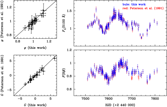
Figure 1.— Intercalibration of the RM data of NGC 5548 from the year 1989 extracted from Peterson et al. (1991). Left panels: comparison of the intercalibration factors $\varphi$ (top) and $G$ (bottom) derived in this work with those from Peterson et al. (1991). The unit of $G$ is $10^{-15}~{}{\rm erg~{}s^{-1}~{}cm^{-2}~{}\text{\AA}^{-1}}$. Solid lines represent the equality of the two results. Right panels: intercalibrated light curves of the 5100 Å continuum (top) and broad H$\beta$ emission line (bottom). The continuum and H$\beta$ fluxes are in units of $10^{-14}~{}{\rm erg~{}s^{-1}~{}cm^{-2}~{}\text{\AA}^{-1}}$ and $10^{-12}~{}{\rm erg~{}s^{-1}~{}cm^{-2}}$, respectively. The light curves from Peterson et al. (1991) are superposed for comparison.

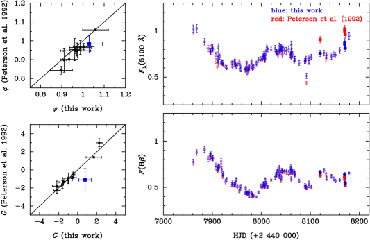
Figure 2.— Same as Figure 1 but for the RM data from the year 1990 extracted from Peterson et al. (1992). Squares highlighted in blue in the left panels represent the intercalibration constants for set “K”, where the previous method encountered difficulties obtaining reliable intercalibration in Peterson et al. (1992). Solid points in the right panels highlight the intercalibrated fluxes for set “K” in this work (in blue) and in Peterson et al. (1992) (in red).

3.1. Year 1989

In the year 1989, NGC 5548 was monitored by 17 telescopes with various individual apertures. Peterson et al. (1991) grouped these measurements into 20 data sets according to the aperture sizes of the corresponding instruments (see Tables 6-8 therein). For the sake of clarity, in this work, we adopt the data set codes following Peterson et al. (1991) to identify the instruments that obtained the spectrum. Each data set is regarded to be internally homogeneous and the variations due to seeing are subsumed into the measurement uncertainties. Peterson et al. (1991) selected the data set (identified by code “A”) with fairly numerous observations as the reference to gain a reasonable overlap with other data sets. They found that to improve the accuracy of the intercalibration, they needed to compare all the measurement pairs separated by up to 2 days. Therefore, the temporal resolution of their light curves should be degraded to be at least larger than 2 days. Indeed, the average interval between the measurements is 3.1 days and the median interval is 1 day (see Peterson et al. 1991 for details).

In Figure 1, we compare the intercalibration results from our method with those from Peterson et al. (1991). The fractional measurement uncertainties for the continuum and the H$\beta$ fluxes are set uniformly to be 0.040 and 0.035, respectively (Peterson et al. 1991). We find remarkable agreement of our results with those of Peterson et al. (1991), indicating the fidelity of our method. As mentioned above, our method does not degrade the temporal resolution; however, the homogeneous IUE data of NGC 5548 showed evidence that the variability seems to begin to appear on a timescale longer than $\sim$5 days (Peterson et al. 1991). It is no surprise that the light curves of both the continuum and H$\beta$ fluxes are fairly consistent with Peterson et al. (1991)’s results. Nevertheless, the measurement point of the continuum on HJD 2,447,546 that seems anomalously high in Peterson et al. (1991) is now slightly lower in our results, as plotted in the top right panel of Figure 1.

3.2. Year 1990

In the year 1990, NGC 5548 was monitored by 12 telescopes and all the measurements are grouped into 12 data sets by Peterson et al. (1992) (see Tables 5-7 therein). Again, data set “A” was adopted as the reference. The short time scale sampling in this year is not sufficiently good as the year in 1989. Consequently, to obtain reliable intercalibration accuracy, Peterson et al. (1992) adopted different time separations of the measurement pairs for comparison with different data sets. In particular, based on their method, it is impossible to intercalibrate data set “K” because none of its observations are within 5 days of any observations of the other sets. Since the variation of NGC 5548 begins to be notable on a timescale of $\sim 5$ days, Peterson et al. (1992) used the intercalibration constants for the set “K” in Peterson et al. (1991). However, an inspection of the intercalibration constants obtained in Peterson et al. (1991, 1992) clearly shows that the constants are not exactly identical for the same set code. Moreover, while the resulting fluxes of H$\beta$ of set “K” looks quite good, the fluxes of the continuum, highlighted with solid symbols in Figure 2, are unexpectedly high (the measurement HJD 2,448,120 in particular), implying that the intercalibration for set “K” is plausibly doubtful.

We show our intercalibration results for the year 1990 in Figure 2. Again, except for set “K”, there is quite good agreement between the two methods. However, our intercalibrated fluxes of the continuum for set “K” seems much more reasonable and are consistent with the other closely spaced measurements regarding the variation trend. This is because our Bayesian approach is not based on a comparison of the closely spaced measurements but instead looks for the most optimized solution for maximizing the posterior distribution in Equation (10). This permits us to cope with poorly sampled data as in set “K”.

4. Conclusions

We propose a feasible Bayesian method for spectral intercalibration in a joint monitoring campaign based on the assumption of flux constancy of some specified narrow emission line (e.g., [O III] $\lambda 5007$). Compared with the previous empirical method comparing the closely spaced measurement pairs, our new method obviates the requirement for (nearly) contemporaneity of observations and takes into account the measurement errors naturally. The Bayesian approach enables us to perform intercalibration on all the data sets simultaneously and self-consistently regardless of sampling rates, and therefore can cope with poorly sampled data. Application to the RM database of NGC 5548 from the AGN Watch Project shows the fidelity of our method and its capability to yield appropriate intercalibration where the previous method encountered difficulties.

In conclusion we propose a road map for complete spectral calibration in RM campaigns in which one or more emission lines with constant flux are present: first employ the algorithm described by van Groningen & Wanders (1992) to perform relative scaling based on the adopted emission line, which takes into account the zero-point wavelength-calibration errors between individual spectra and resolution differences; and then employ our method to perform intercalibration to correct for the effect of inhomogeneous apertures.

References

- Ai et al. (2013) Ai, Y. L., Yuan, W., Zhou, H., et al. 2013, AJ, 145, 90
- Bentz et al. (2013) Bentz, M. C., Denney, K. D., Grier, C. J., et al. 2013, ApJ, 767, 149
- Blandford & McKee (1982) Blandford, R. D., & McKee, C. F. 1982, ApJ, 255, 419
- Brewer et al. (2011) Brewer, B. J., Treu, T., Pancoast, A., et al. 2011, ApJL, 733, 33
- Czerny et al. (1999) Czerny, B., Schwarzenberg-Czerny, A., & Loska, Z. 1999, MNRAS, 303, 148
- Denney et al. (2010) Denney, K. D., Peterson, B. M., Pogge, R. W., et al. 2010, ApJ, 721, 715
- Dexter & Agol (2011) Dexter, J., & Agol, E. 2011, ApJL, 727, L24
- Grier et al. (2012) Grier, C. J., Peterson, B. M., Pogge, R. W., et al. 2012, ApJ, 755, 60
- Kelly et al. (2009) Kelly, B. C., Bechtold, J., & Siemiginowska, A. 2009, ApJ, 698, 895
- Kelly et al. (2011) Kelly, B. C., Sobolewska, M., & Siemiginowska, A. 2011, ApJ, 730, 52
- Kozłowski et al. (2010) Kozłowski, S., Kochanek, C. S., Udalski, A., et al. 2010, ApJ, 708, 927
- Li et al. (2013) Li, Y.-R., Wang, J.-M., Ho, L. C., Du, P., & Bai, J.-M. 2013, ApJ, 779, 110
- Liu (2001) Liu, J. S. 2001, Monte Carlo Strategies in Scientific Computing (New York: Springer)
- MacLeod et al. (2010) MacLeod, C. L., Ivezić, Ž., Kochanek, C. S., et al. 2010, ApJ, 721, 1014
- MacLeod et al. (2012) MacLeod, C. L., Ivezić, Ž., Sesar, B., et al. 2012, ApJ, 753, 106
- Meusinger & Weiss (2013) Meusinger, H., & Weiss, V. 2013, A&A, 560, A104
- Mushotzky et al. (2011) Mushotzky, R. F., Edelson, R., Baumgartner, W., & Gandhi, P. 2011, ApJL, 743, L12
- Noble & Krolik (2009) Noble, S. C., & Krolik, J. H. 2009, ApJ, 703, 964
- Pancoast et al. (2012) Pancoast, A., Brewer, B. J., Treu, T., et al. 2012, ApJ, 754, 49
- Pecháček et al. (2013) Pecháček, T., Goosmann, R. W., Karas, V., Czerny, B., & Dovčiak, M. 2013, A&A, 556, A77
- Peterson (1993) Peterson, B. M. 1993, PASP, 105, 247
- Peterson et al. (1992) Peterson, B. M., Alloin, D., Axon, D., et al. 1992, ApJ, 392, 470
- Peterson et al. (1991) Peterson, B. M., Balonek, T. J., Barker, E. S., et al. 1991, ApJ, 368, 119
- Peterson et al. (2002) Peterson, B. M., Berlind, P., Bertram, R., et al. 2002, ApJ, 581, 197
- Peterson et al. (2004) Peterson, B. M., Ferrarese, L., Gilbert, K. M., et al. 2004, ApJ, 613, 682
- Peterson et al. (1995) Peterson, B. M., Pogge, R. W., Wanders, I., Smith, S. M., & Romanishin, W. 1995, PASP, 107, 579
- Reynolds & Miller (2009) Reynolds, C. S., & Miller, M. C. 2009, ApJ, 692, 869
- Rybicki & Press (1992) Rybicki, G. B., & Press, W. H. 1992, ApJ, 398, 169
- Ulrich et al. (1997) Ulrich, M.-H., Maraschi, L., & Urry, C. M. 1997, ARA&A, 35, 445
- van Groningen & Wanders (1992) van Groningen, E., & Wanders, I. 1992, PASP, 104, 700
- Zu et al. (2013) Zu, Y., Kochanek, C. S., Kozłowski, S., & Udalski, A. 2013, ApJ, 765, 106
- Zu et al. (2011) Zu, Y., Kochanek, C. S., & Peterson, B. M. 2011, ApJ, 735, 80
- Zuo et al. (2012) Zuo, W., Wu, X.-B., Liu, Y.-Q., & Jiao, C.-L. 2012, ApJ, 758, 104