Low-complexity Decoding is Asymptotically Optimal in the SIMO MAC

Abstract

A single input multiple output (SIMO) multiple access channel, with a large number of transmitters sending symbols from a constellation to the receiver of a multi-antenna base station, is considered. The fundamental limits of joint decoding of the signals from all the users using a low complexity convex relaxation of the maximum likelihood decoder (ML, constellation search) is investigated. It has been shown that in a rich scattering environment, and in the asymptotic limit of a large number of transmitters, reliable communication is possible even without employing coding at the transmitters. This holds even when the number of receiver antennas per transmitter is arbitrarily small, with scaling behaviour arbitrarily close to what is achievable with coding. Thus, the diversity of a large system not only makes the scaling law for coded systems similar to that of uncoded systems, but, as we show, also allows efficient decoders to realize close to the optimal performance of maximum-likelihood decoding. However, while there is no performance loss relative to the scaling laws of the optimal decoder, our proposed low-complexity decoder exhibits a loss of the exponential or near-exponential rates of decay of error probability relative to the optimal ML decoder.

I Introduction

Although the capacity-achieving techniques of superposition coding at the encoder and joint decoding at the decoder [1] promise significantly higher capacity for multiuser networks, such sophisticated coding schemes often suffer from practical challenges. Thus the simpler orthogonal schemes to separate users either in time (TDMA), space (sectorization in cellular networks) or frequency (FDMA) have remained in widespread use. Moreover, the capacity benefits of the optimal scheme over orthogonalizing schemes like time-division have been shown to be negligible in some regimes such as under asymptotically low-power or for asymptotically many users ([2],[3]).

In this work we consider a multiple access setting where an asymptotically large number of transmitting users communicate in a rich scattering environment with a single multi-antenna base station. We look at transmitting schemes which do not employ coding, but instead transmit symbols from the BPSK constellation and rely on the diversity inherent in a large system to achieve reliability. Such a setting may model sensor networks or general distributed networks with energy/processing power limitations at the transmitters (which may preclude sophisticated coding schemes) and centralized receivers. A similar setting was considered in the companion paper [4], where it was shown that using the optimal maximum likelihood (ML) decoder, the decoding can be made arbitrarily reliable for an arbitrarily small number of receiver antennas per transmitter, provided that the number of transmitters is large enough. A similar setup was also considered in [5] where a relaxation of the maximum likelihood decoder was shown to be asymptotically reliable (i.e. the probability of error vanishing to zero) in the number of transmitters, provided that the number of receiver antennas is more than the number of transmitters.

In this work, we analyze the same low-complexity decoder proposed in [5] and modify it to handle underdetermined systems, i.e. systems where the number of receiver antennas is less than the number of transmitter antennas. In particular we consider the decoder obtained by expanding the search over possible symbols to intervals instead of discrete points and then quantizing the output of the interval search to the nearest constellation point. This relaxation of the search over integer points to search over intervals allows more efficient (polynomial time) decoding, but may not be unique in the regime of underdetermined systems (because of the non-trivial null space for a wide channel matrix). Thus the above procedure yields a non-singleton solution set in general. We propose a family of randomization techniques and show that they can return provably good estimates from this solution set. Henceforth we will refer to this decoding technique as the randomized interval search and quantize (r-ISQ) decoder. We obtain analytical bounds on the performance of the r-ISQ decoder and show that reliable decoding (in a sense made precise in the later sections) is possible in the asymptotic limit of a large number of transmitters and receivers, with the per-transmitter number of receiver antennas being held constant at any arbitrary positive value. Using the same techniques used in the proof however, the per-transmitter number of receive antennas can be shown to be arbitrarily close to the theoretically optimal scaling derived e.g. in [6],[4].

The rest of the paper is organized as follows. We first present the system model and describe the optimal decoder and the r-ISQ decoder. We then describe a bound on the error probability of this decoder. Asymptotic analyses of these bounds are then presented.

II System Model

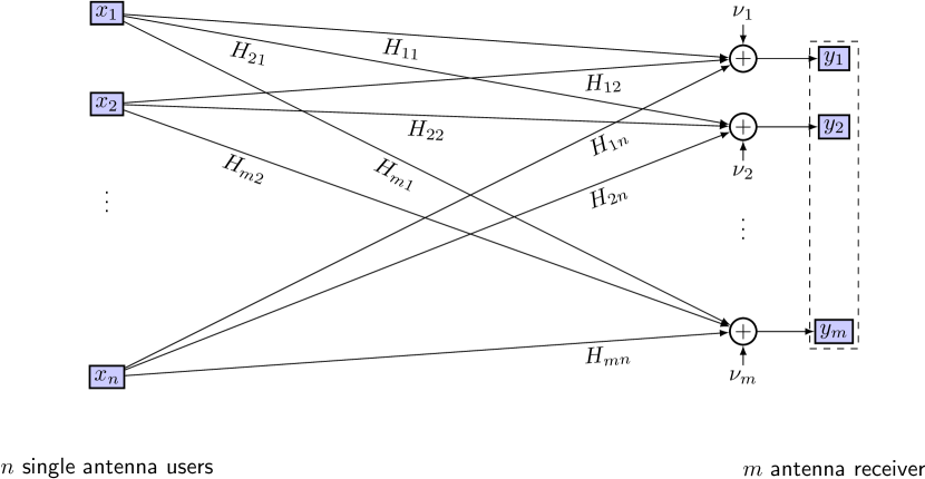
Figure 1: System model

Our system model is depicted in Figure 1. We have an uplink system with $n$ single-antenna transmitters and an $m$ antenna receiver. The channel matrix $\mathbf{H}\in\mathbb{R}^{m\times n}$ is chosen to model a rich scattering environment, and the entries are assumed to be drawn i.i.d. from $\mathcal{N}(0,1)$. The $k^{th}$ column of $\mathbf{H}$ is denoted as $\mathbf{h_{k}}\in\mathbb{R}^{m}$. Thus

$$\mathbf{H}=\begin{pmatrix}\mathbf{h_{1}}&\mathbf{h_{2}}&\ldots&\mathbf{h_{n-1}}&\mathbf{h_{n}}\end{pmatrix}.$$

We also assume that the users do not cooperate with each other and that they transmit symbols from the standard unit energy BPSK constellation. The components of the noise at the receiver ($\nu$ ) are assumed to be i.i.d. $\mathcal{N}(0,\sigma^{2})$. The received signal at the multi-antenna receiver is then

$$\mathbf{y}=\mathbf{Hx}+\bm{\nu}.$$ (1)

The vector $\mathbf{x}\in\{-1,+1\}^{n}$, which consists of the transmitted symbols from the $n$ users, is referred to as the n-user codeword to indicate that the receiver decodes the block of n-user constellation points simultaneously. We further assume that the receiver has perfect channel state information (CSI) and that the transmitters have no CSI.

III Previous work and results

We now describe a few observations and results about the performance limits of this system. These results, derived in [6], [4], assume that the receiver employs ML decoding, i.e. it returns

$$\mathbf{\hat{x}}=\operatorname{argmin}_{\mathbf{x}\in\{-1,+1\}^{n}}||\mathbf{y}-\mathbf{Hx}||^{2}.$$ (2)

With this decoder it has been shown that in the limit of a large number of transmitters the following holds:

Theorem 1.

Under ML decoding, there exists a $d>0$ such that for all sufficiently large $n$, the probability of error in decoding the n-user codeword satisfies

$${P_{\mathrm{error}}}\leq 2^{-dn}.$$

In other words the probability of decoding a particular user’s transmitted symbol in error decreases exponentially with the number of users, even though the users do not employ any coding across time.

A critical component in [6], [4] to achieve this asymptotic result is the use of ML decoding. In this work we investigate whether we can achieve reliability even with lower-complexity decoders. In particular, we ask whether an efficient polynomial time decoder can realize an asymptotically vanishing probability of error, as was the case with the ML decoder.

A common approach to relax hard combinatorial optimization problems (such as ML decoding) is the technique of expanding the search space from discrete points to intervals or regions [7]. Motivated by this idea, we consider a convex relaxation of the maximum likelihood decoder search as follows:

$$\mathbf{\hat{x}}=\operatorname{sgn}(\operatorname{argmin}_{\mathbf{x}\in[-1,+1]^{n}}||\mathbf{y}-\mathbf{Hx}||^{2}).$$ (3)

In the above $\operatorname{sgn}(\mathbf{x})$ for $\mathbf{x}\in\mathbb{R}^{n}$ refers to the vector obtained by the coordinatewise application of the signum function defined below for a scalar $x$.

$$\operatorname{sgn}(x)=\begin{cases}1&\text{ if $x>0$}.\\ -1&\text{ otherwise}.\end{cases}$$

The modified decoder in (3) expands the search for a valid n-user codeword to the interval $[-1,1]$ per dimension and then quantizes it to integer values afterwards, hence we call it an ISQ decoder. This idea of relaxing an integer program to a box-constrained program is a well known technique and has been studied in different settings, e.g. in [8], [9], where different asymptotic properties of this decoder are established. While some of the results (especially the characterization of the null space of Gaussian random matrices [8], and the behaviour of approximate message passing (AMP) type algorithms [9] with the box constraints) from these works do give us insights into the expected behaviour of the box constrained decoder in some regimes (e.g. $\frac{m}{n}>0.5$ with BPSK transmissions), the regime of an arbitrarily small fraction of the per-transmitter number of receiver antennas is still not fully characterized. In fact, for the AMP decoder, it can be shown that if $\frac{m}{n}<0.5$, the number of symbol errors in the decoded block would be $\Theta(n)$, i.e. the number of incorrectly decoded symbols is linear in the number of transmitting users. We consider a slight modification of the box-constrained decoder and with this modification, are able to show asymptotic reliability in a sense made precise below.

Note that in the regime where the channel matrix is underdetermined (i.e. $m<n$ ) the above procedure may not give a unique solution. If an n-user codeword $\hat{\mathbf{x}}$ is a solution, then any codeword of the form $\hat{\mathbf{x}}+\bm{Z\beta}$ is also a solution. Here $\mathbf{Z}$ is a basis for the right null space of $\mathbf{H}$, i.e. $\mathbf{Z}$ is such that $\mathbf{H}\mathbf{Z}=\mathbf{0}$ and $\bm{\beta}\in\mathbb{R}^{(1-\alpha)n}$. Thus the ISQ decoder, in this case, cannot uniquely specify a solution by itself. It would, in general, give an affine subspace as a solution. In order to specify a unique solution, we propose a randomization step (randomized ISQ or r-ISQ). Specifically, we propose a family of distributions and show that, for estimates drawn according to this general family of distributions, we can achieve reliability in a sense which is made precise in the following sections. We further show that it is possible to sample efficiently from a member of this family of distributions. For specificity let us consider the following decoder.

$$\text{r-ISQ:}\,\mathbf{\hat{x}}=\operatorname{sgn}(\operatorname{argmin}_{\mathbf{x}\in S}||\mathbf{x_{r}}-\mathbf{x}||_{\infty}).$$

In the above $S=\{\mathbf{x}:\mathbf{x}\in\operatorname{argmin}_{\mathbf{z}}||\mathbf{y}-\mathbf{Hz}||\}$, and $\mathbf{x_{r}}\sim\operatorname{Unif}([-1,1]^{n})$. Since both $\mathbf{x_{r}}$ and $S$ can be computed efficiently (in polynomial time, for reasons discussed in later sections), we see that there is an efficient algorithm to achieve asymptotic reliability without employing coding.

However there is a performance hit, relative to ML decoders, when we move to r-ISQ decoders. This is in terms of the rate of decay of the error probability with the number of transmitting users. Although the error probability seen by each user vanishes to zero, we do not have an upper bound for the probability of having at least one symbol error in the n-user codeword, which is in contrast to ML, where the block error probability decays exponentially. This lack of exponential decay with the simpler decoder is primarily due to the self interference due to the search over intervals. Thus, in particular, we do seem to lose the exponential fall off in the probability of error that is achieved with the ML decoder. However, the number of symbol errors in the decoded block in the asymptotic limit is at most sub linear, i.e. the probability that a constant fraction of the transmitter symbols are incorrectly decoded can be made arbitrarily small for a large enough system size. Defining $P_{e}^{k^{\prime}}$ to be the probability of incorrectly decoding at least $k^{\prime}n$ out of $n$ transmitted symbols, the following states a bound on $P_{e}^{k^{\prime}}$.

Theorem 2.

Under r-ISQ decoding, for $m=\alpha n$ , $\alpha>0$ and any constant $k>0$, there exists a $d>0$ such that for all sufficiently large $n$,

$$P_{e}^{k}\leq 2^{-dn\log n}.$$

We mention that the same proof techniques used to establish the above result can also be used to get sharper bounds, i.e. for $k=\frac{1}{n^{\gamma}}$ for some $0<\gamma<1$. Thus the per-user error probability is asymptotically less than $\frac{1}{n^{\gamma}}$. Also, while in this section we focus on the case where the ratio ($\alpha$) of the number of receiver antennas to the number of transmitter antennas is constant, we point out that the same techniques continue to hold even for

$$\alpha_{n}=\frac{1}{(\log n)^{\xi}},\xi<1.$$

By making $\xi$ close to $1$ we see that we can come arbitrarily close to the optimal scaling established for the ML decoder in [6]. Thus we see that by exploiting the diversity (richness in the scattering environment), one can not only get arbitrarily reliable communication in different asymptotic regimes (in this case for a large number of transmitters) without employing coding or ML decoders, but can also achieve optimal scaling for the per transmitter number of receiver antennas.

We now use the bound in Theorem 2 to bound the probability of symbol error seen by each transmitter.

Theorem 3.

The probability of error with the r-ISQ decoder seen by any transmitting user vanishes in the limit of an asymptotically large number of transmitters, with the per-transmitter number of receive antennas being any constant $\alpha>0$.

The remainder of this paper discusses the proofs of Theorems 2 and 3 and points out suitable generalizations using the same proof techniques.

IV An Upper Bound on the Decoding Error

We first present an upper bound on the probability of decoding error. Most of the steps described in this are similar to what was used in [5], modified to take into account the fact that there is a non-trivial null space (so the solution set in general may not be unique). We look at the pairwise error probability of mistaking the transmitted codeword with one differing in $k^{\prime}n$ symbols. For (3), the probability of mistaking a codeword $\mathbf{x_{0}}$ for another differing in $i$ symbol positions is given by

$$P_{e,\mathbf{b_{i}}} \leq Q\left(\min_{{\mathbf{x}}:\operatorname{supp}(\operatorname{sgn}(\mathbf{x})-\mathbf{x_{0}})=\mathbf{b_{i}}}\frac{||\mathbf{H}(\mathbf{x}-\mathbf{x_{0}})||}{2\sigma}\right).$$ (4)

Here $Q(x)=\frac{1}{\sqrt{2\pi}}\int_{x}^{\infty}e^{-x^{2}/2}dx$, $\mathbf{b_{i}}$ is a vector of size $i$ whose entries are positions where the codewords differ (arranged in increasing order), and $\mathbf{b_{i}}(j)$ is the $j^{th}$ symbol position where the codewords differ. We point out here that $\mathbf{b_{i}}$ has a one-to-one correspondence with a subset of $\{1,\ldots,n\}$ of cardinality $i$. $||\mathbf{x}||_{0}$ refers to the number of non-zero entries in $\mathbf{x}$. $\operatorname{supp}(\mathbf{x})$ refers to the support (i.e. locations of the non-zero entries of vector $\mathbf{x}$).

Note that the error probability above is independent of which $\mathbf{x_{0}}$ is chosen, when averaged over the distribution of $\mathbf{H}$. Hence, choosing $\mathbf{x_{0}}=-\mathbf{1}$, we note that the last expression can be rewritten as follows.

$$P_{e,\mathbf{b_{i}}}\leq Q\left(\min_{\begin{subarray}{c}1\leq c_{j}\leq 2\,\forall j\in\mathbf{b_{i}}\\ 0\leq c_{j}\leq 1\,\forall j\in\mathbf{b_{i}}^{c}\end{subarray}}\frac{||\sum_{j=1}^{n}c_{j}\mathbf{h_{b_{i}(j)}}||}{2\sigma}\right)$$

$$\overset{(a)}{\leq}\frac{1}{2}\exp{\left(-\min_{\begin{subarray}{c}1\leq c_{j}\leq 2\,\forall j\in\mathbf{b_{i}}\\ 0\leq c_{j}\leq 1\,\forall j\in\mathbf{b_{i}}^{c}\end{subarray}}\frac{||\sum_{j=1}^{n}c_{j}\mathbf{h_{b_{i}(j)}}||^{2}}{8\sigma^{2}}\right)}$$ (5)

where (a) follows because $Q(x)\leq\frac{1}{2}\exp(\frac{-x^{2}}{2})$. We observe now that (5) averaged over the channel realizations is independent of the particular subset of symbols that are decoded in error and depends only on the size $i$ of such a subset. Let’s call this averaged probability of error $P_{i}$. Thus we have

$$P_{i}\triangleq E_{\mathbf{H}}e^{\left(-\min_{\begin{subarray}{c}1\leq c_{j}\leq 2\,\forall\,j\in\{1,\ldots,i\}\\ 0\leq c_{j}\leq 1\,\forall j\in\{i+1,\ldots,n\}\end{subarray}}\frac{||\sum_{j=1}^{n}c_{j}\mathbf{h_{j}}||^{2}}{8\sigma^{2}}\right)}.$$

If $P_{e}^{k^{\prime}}$ is the probability of error of decoding at least $k^{\prime}n$ transmitter symbols incorrectly, and $S_{i}$ refers to the set of all vectors representing subsets of size $i$ from $\{1,\ldots,n\}$, then a union bound for the error probability is

$$P_{e}^{k^{\prime}} \leq \sum_{k^{\prime}n\leq i\leq n}\sum_{\mathbf{b}\in S_{i}}\frac{1}{2}P_{i}$$ (6)

$$\leq \sum_{k^{\prime}n\leq i\leq n}\binom{n}{i}\frac{1}{2}P_{i}.$$ (7)

Note that, by the symmetry of the system, the probability of error $P_{e}$ seen by each transmitting user is upper bounded by

$$P_{e}\leq k^{\prime}+P_{e}^{k^{\prime}}.$$

We show that for any small $k^{\prime}$, there exists a large enough system size for which $P_{e}^{k^{\prime}}$ becomes exponentially small, even with a convex decoder of much lower complexity. This will establish Theorem 3.

V Asymptotic analysis of the upper bound

We first prove bounds on the exponent appearing in the bound for $P_{e,\mathbf{b_{i}}}$ in (5). Specifically, we look at (ignoring a constant scaling of $8\sigma^{2}$)

$$\min_{\begin{subarray}{c}1\leq c_{j}\leq 2\,\forall j\in\{1,\ldots,i\}\\ 0\leq c_{j}\leq 1\,\forall j\in\{i+1,\ldots,n\}\end{subarray}}||\sum_{j=1}^{n}c_{j}\mathbf{h_{j}}||^{2}.$$

Before we describe the proof, we define the ($\epsilon,\bm{\delta}$)-grid inside the hypercube $[-1,+1]^{n}$, for some $0<\epsilon<0.25$. This grid is simply the set of points

$$\mathcal{G}_{n,\epsilon,\bm{\delta}}=\{\mathbf{x}:x_{i}\bmod\epsilon=\delta_{i},-1\leq x_{i}\leq 1\,\,\forall i\}.$$

As an illustration, for $\bm{\delta}=\bm{0}$, it may be rewritten as

$$\mathcal{G}_{n,\epsilon,\bm{\delta}}=\{-1,-1+\epsilon,\ldots,1-\epsilon,1\}^{n}.$$

if $\frac{1}{\epsilon}\in\mathbb{N}$.

We now introduce the $(\epsilon,\bm{\delta})$-ISQ decoder, so named because it replaces the interval search in the ISQ decoder by an ($\epsilon,\bm{\delta}$)-grid search:

$$\text{$(\epsilon,\bm{\delta})$-ISQ:}\,\mathbf{\hat{x}}_{\epsilon,\bm{\delta}}=\operatorname{sgn}(\operatorname{argmin}_{\mathbf{x}\in\mathcal{G}_{n,\epsilon,\bm{\delta}}}||\mathbf{y}-\mathbf{Hx}||^{2}).$$

The $(\epsilon,\bm{\delta})$-grid error probabilities are defined similar to the definitions for the ISQ decoder in the previous section, and are indicated by an $\epsilon,\bm{\delta}$ subscript. We now collect some observations about the grid error probabilities and use a union bounding argument for $P_{e,\mathbf{b_{i}},\epsilon,\bm{\delta}}$. Some of these results for the grid error probabilities have already been derived in [5] and have been reproduced here for completeness and continuity of presentation. We require the following lemma about the negative of the exponent in the error probability $P_{e,\mathbf{b_{i}},\epsilon,\bm{\delta}}$:

$$\min_{\begin{subarray}{c}c_{j}\in[1,2],c_{j}\bmod\epsilon=\delta_{j}\,\forall j\in\{1,\ldots,i\}\\ c_{j}\in[0,1],c_{j}\bmod\epsilon=\delta_{j}\,\forall j\in\{i+1,\ldots,n\}\end{subarray}}||\sum_{j=1}^{n}c_{j}\mathbf{h_{j}}||^{2}.$$

Lemma 1.

For any $i>k^{\prime}n$, there exists an $n_{0}$ and an $a>0$, such that for all $n>n_{0}$,

$$P(||\sum_{j=1}^{n}c_{j}\mathbf{h_{j}}||^{2}<an\log n)\leq\exp(-an\log n).$$

Proof.

We can show this using Markov’s inequality. Let $a_{1}=\frac{\alpha}{4}.$ Then

$$P(||\sum_{j=1}^{n}c_{j}\mathbf{h_{j}}||^{2}<a_{1}n\log n)$$ (12)

$$= P(\exp(-t||\sum_{j=1}^{n}c_{j}\mathbf{h_{j}}||^{2})>\exp(-ta_{1}n\log n))$$

$$\overset{(a1)}{\leq}\exp(ta_{1}n\log n)E\exp(-t||\sum_{j=1}^{n}c_{j}\mathbf{h_{j}}||^{2})$$

$$\overset{(a2)}{=}\exp(ta_{1}n\log n)(1+2t\sum_{j}c_{j}^{2})^{(-\alpha n/2)}$$

$$\overset{(b)}{\leq}\exp(ta_{1}n\log n)(1+2tk^{\prime}n)^{(-\alpha n/2)}$$

$$\overset{(c)}{\leq}\exp(-\tilde{a}n\log n)\,\,\text{ for large enough n}.$$

In the above $(a1)$ follows from Markov’s inequality, $(a2)$ follows from the moment generating function of a chi-squared random variable, $(b)$ follows from the fact that for at least $k^{\prime}n$ errors,

$$\sum_{j}c_{j}^{2}\geq k^{\prime}n,$$

and $(c)$ follows by choosing $t=1$, and defining e.g. $\tilde{a}=\frac{\alpha}{4}.$ Defining $a=\min(a_{1},\tilde{a})=\frac{\alpha}{4}$, we get the claim in the lemma. Thus the claim is established for $\mathbf{H}$ with $\mathcal{N}(0,1)$ entries.

∎

By observing that for a positive r.v., $P(x<d_{0})<\exp(-d_{0})$ implies

$$E(\exp(-x))$$ (13)

$$\leq \exp(-d_{0})+(1-\exp(-d_{0}))\exp(-d_{0})$$ (14)

$$\leq 2\exp(-d_{0}),$$ (15)

we get that

$$P_{i,\epsilon,\bm{\delta}} \leq E(\exp(-||\sum_{j=1}^{n}c_{j}\mathbf{h_{j}}||^{2}))$$ (16)

$$\leq \exp(-an\log n)\,\,\text{ for large enough n}.$$ (17)

The probability of the event that there are at least $k^{\prime}n$ symbols that are decoded incorrectly can then be union bounded as follows.

$$P_{e,\epsilon,\bm{\delta}}^{k^{\prime}} \leq \sum_{i=k^{\prime}n}^{n}\binom{n}{i}\left(\frac{1}{\epsilon}\right)^{n}P_{i,\epsilon,\bm{\delta}}$$

$$\overset{(d1)}{\leq} n2^{n(\max_{k^{\prime}n\leq i\leq n}H_{2}(\frac{i}{n})-\log(\epsilon)-a\log n)}\,\,\text{ for }$$

$$a>0 n$$ and large enough

$$\overset{(d2)}{\leq} 2^{-an\log n}\,\,\text{for a large enough n}.$$

In the above,

$$H_{2}(x)=-x\log x-(1-x)\log(1-x).$$

$(d1)$ follows by noting that

$$\binom{n}{i}\leq 2^{H_{2}(i/n)}$$

and $(d2)$ follows from the observation that $H_{2}(\cdot)$ is bounded above by a constant. We now note that by introducing an arbitrary distribution $f(\bm{\delta})$ on $\bm{\delta}$, i.e. randomizing the grid, there would be a distribution induced on $\bm{\hat{x}}_{\epsilon,\bm{\delta}}$. Let’s call that $\hat{f}(\bm{\hat{x}}_{\epsilon,\bm{\delta}})$. Thus statements about the probability of error associated with $\mathbf{\hat{x}}_{\epsilon,\bm{\delta}}$ would continue to hold even for samples $\mathbf{y}$ drawn from $\hat{f}(\mathbf{y})$. Note that sampling from this distribution may still be of exponential complexity. Let’s call this decoder the r-$(\epsilon,\bm{\delta})$ ISQ decoder, where r stands for randomized.

We now relate the solution from the search over the randomized $(\epsilon,\bm{\delta})$-grid $\mathcal{G}_{n,\epsilon,\bm{\delta}}$ (i.e. the output of the r-$(\epsilon,\bm{\delta})$ ISQ decoder) to the solution ($\hat{\mathbf{x}}$) of the r-ISQ decoder. Note that, in general, the ISQ decoder will not be unique and there is always an uncertainty due to the right null space of $\mathbf{H}$. Thus if the objective function in the ISQ decoder attains its infimum at $\hat{\mathbf{x}}$, then it will also attain the same infimum at all points of the following solution set

$$S=\{\mathbf{x}:\mathbf{x}=\hat{\mathbf{x}}+\mathbf{Z}\bm{\beta},\mathbf{HZ}=\bm{0},\bm{\beta}\in\mathbb{R}^{(1-\alpha)n}\}.$$

We show next that a certain randomized choice of solution from this solution set will be “good”. Before that however, we introduce some notation. Let the projection of any vector $\mathbf{y}$ on any set $A$ be defined by

$$P_{A}(\mathbf{y}) = \operatorname{argmin}_{\mathbf{x}\in A}||\mathbf{y}-\mathbf{x}||_{\infty}.$$ (20)

Note that this can be computed efficiently (using interior point algorithms) if $A$ is an affine subspace. Thus given $\mathbf{\hat{x}}_{\epsilon,\bm{\delta}}$, one can compute $P_{S}(\mathbf{\hat{x}}_{\epsilon,\bm{\delta}})$ efficiently. This is simply the projection of the solution of the r-$(\epsilon,\bm{\delta})$-ISQ decoder on the solution space $S$ of the ISQ decoder. Before we proceed we observe a certain property that this projection enjoys.

Lemma 2.

There is at least one point of the solution set $S$ of the ISQ within the $\epsilon-l_{\infty}$ ball around $\hat{\mathbf{x}}_{\epsilon,\bm{\delta}}$, i.e., $||\mathbf{\hat{x}}_{\epsilon,\bm{\delta}}-P_{S}(\mathbf{\hat{x}}_{\epsilon,\bm{\delta}})||_{\infty}\leq\epsilon$.

Proof.

We can show this by contradiction. If the claim is false, we would have that the function $g(\mathbf{x})=||\mathbf{y}-\mathbf{H}\mathbf{x}||^{2}$ is strictly convex over the hypercube $\{\mathbf{x}:||\mathbf{x}-\mathbf{x}_{\epsilon,\bm{\delta}}||_{\infty}\leq\epsilon\}$, with $S$ lying totally outside the hypercube. By observing that, in such a case, one of the vertices will have a smaller value for $g(\mathbf{x})$ than $g(\mathbf{\hat{x}}_{\epsilon,\bm{\delta}})$, we arrive at a contradiction. ∎

Figure 2: $(\epsilon,\bm{\delta})$-grid for $n=3,\alpha=2/3$ (dotted grid with gray grid points) for a $\mathbf{H}\in\mathbb{R}^{2\times 3}$

Thus projecting to the solution space $S$ does not change any entry of the vector $\mathbf{\hat{x}}_{\epsilon,\bm{\delta}}$ by more than $\epsilon$. Since $\epsilon<0.25$, if $|{\mathbf{\hat{x}}}_{\epsilon,\bm{\delta},i}|>\epsilon$, the sign of the corresponding entry of $P_{S}({\mathbf{\hat{x}}}_{\epsilon,\bm{\delta}})$ would also be the same as that of $\mathbf{\mathbf{\hat{x}}}_{\epsilon,\bm{\delta}}$. The remaining part of the proof is to establish that the sampling of the point $\mathbf{y}=P_{S}({\mathbf{\hat{x}}}_{\epsilon,\bm{\delta}})$ according to distribution $\hat{f}_{S}(\mathbf{y})$ can be done efficiently, i.e. with polynomial complexity (this, in general, is not true for arbitrary multivariate distributions, i.e. [10]). This, together with the fact that the $|{\mathbf{\hat{x}}}_{\epsilon,\bm{\delta},i}|$ is less than $\epsilon$ at most at a sublinear number of coordinates $i$ with overwhelming probability, establishes the fact that $P_{S}({\mathbf{\hat{x}}}_{\epsilon,\bm{\delta}})$ differs from $\mathbf{x_{0}}$ in at most a sublinear number of positions with high probability.

We now relate this randomized projection to the solution of the r-ISQ decoder. This simply takes the affine subspace that is a solution to the ISQ decoder and projects a random point inside the hypercube on it. Thus

$$\text{r-ISQ:}\mathbf{\hat{x}}=P_{S}(\mathbf{x_{r}}),\mathbf{x_{r}}\sim\text{Unif}([-1,1]^{n})$$ (21)

where $S$ is the solution set of the ISQ decoder. Note that since $S$ is affine and the sampling is uniform, both can be done efficiently. We now show that the estimate from this decoder is equal to that of the r-$(\epsilon,\bm{\delta})$-ISQ decoder for a particular choice of $f(\bm{\delta})$. This follows from the observation that any distribution on $\mathbf{x_{r}}$ would induce a distribution on $S$. This distribution belongs to the family of distributions of the form $\hat{f}_{S}$ induced by a distribution $f(\bm{\delta})$ on $\bm{\delta}$ because the mapping $P_{S}(\mathbf{\hat{x}}_{\epsilon,\bm{\delta}})$ from $\bm{\delta}$ to $S$ is onto (surjective). Also, by following the same union bounding technique used to bound $P_{e,\epsilon,\bm{\delta}}^{k^{\prime}}$, we get that, for any $k^{{}^{\prime\prime}}>0$, the probability that $\hat{\mathbf{x}}_{\epsilon,\bm{\delta}}$ has greater than or equal to $k^{{}^{\prime\prime}}n$ entries that are close to zero, (i.e. either $\delta_{i}-\epsilon,\delta_{i},$ or $\delta_{i}+\epsilon$) is upper bounded by $\exp(-d_{1}n\log n)$, for some $d_{1}>0$. Let

$$d_{2}=\min(d_{1},a).$$

Thus we conclude that for a large enough $n$, with probability at least $1-2\exp(-d_{2}n\log n)$, the signs of $P_{S}(\mathbf{x_{r}})$ will match the signs of $\mathbf{x_{0}}$ (i.e. the correct $n$-user codeword) in at least $(1-k^{{}^{\prime\prime}}-k^{{}^{\prime}})n$ positions. By choosing $k^{{}^{\prime}}$ and $k^{{}^{\prime\prime}}$ small enough we see that the number of mismatches is sublinear in the number of transmitting users with overwhelming probability. The proof of Theorem 2 is now complete. ∎

To prove Theorem 3, we note that, by the symmetry of the system, the error probability $P_{e}$ seen by each transmitter is the same. Thus given any target symbol error rate (SER) $\epsilon_{1}>0$, we can choose $k<\epsilon_{1}/2$ in Theorem 2. Then there exists an $n_{0}$ depending on $k$ such that

$$P_{e}^{k}\leq 2^{-dn\log n}\leq\frac{\epsilon_{1}}{2}\,\,\forall n>n_{0}.$$

Then, assuming independent (both temporally and spatially) channel realizations, we get that the expected number of errors $E(N_{e})$ seen by all transmitters in $t$ single shot transmissions satisfies

$$E(N_{e}) \leq nkt+n(1-k)P_{e}^{k}t$$ (22)

$$\text{or }\frac{E(N_{e})}{t} \leq n\epsilon_{1}\,\,\text{for $n$ large enough.}$$ (23)

Dividing both sides by $n$ we get that the per-transmitter error probability $P_{e}$ can be made smaller than $\epsilon_{1}$ for a large enough $n$. The proof is now complete.

We now comment on some of the differences from the analysis in [5]. One complication is introduced by the fact that the null space is not empty. Thus the properties of the null space will affect the behaviour of the resulting estimate. In particular, as seen in [9], there does exist a “bad solution”, in the sense that it differs from the correct solution in $\Theta(n)$ symbols. However, we are able to establish that in order to reliably “clean up” the solution from the ISQ decoder, a random sample would be sufficient. Moreover, it is possible to sample efficiently from this solution set. Thus although computing $\hat{\mathbf{x}}_{\epsilon,\bm{\delta}}$ (and thereby $P_{S}(\hat{\mathbf{x}}_{\epsilon,\bm{\delta}})$) has exponential complexity, sampling from $\hat{f}_{S}$ does not. We then propose a simple randomized solution, and show that this belongs to the family of distributions just mentioned. Note that both the sampling and the projection operation can be done efficiently in polynomial time. We show that the distribution on the resulting estimate $\tilde{f_{S}}(\bm{\tilde{y}})$ is within the family of distributions $\{\hat{f}_{S}(\bm{y}):\bm{y}=P_{S}(\hat{\mathbf{x}}_{\epsilon,\bm{\delta}}),\bm{\delta}\sim f(\bm{\delta})\}$. This concludes the proof. ∎

VI Extensions

In this section, we point out several extensions to the same ideas that we discussed so far, for more general systems. In particular we focus on the more general kinds of fading distribution, more general constellations, finite blocklength constellations, and faster decay of the probability of error with $n$. We also indicate how the Theorem 3 holds not only for a constant $\alpha>0$, but also for an asymptotically vanishing sequence of $\alpha_{n}$, i.e.

$$\alpha_{n}=\frac{1}{(\log n)^{\xi}}\,\,\textrm{ for }0<\xi<1.$$

VI-A General fading distribution

In the derivation of the proof so far, we assumed i.i.d. $\mathcal{N}(0,1)$ fading for the channel coefficients. We now show how they may be generalized to a much wider class of fading distributions, namely any distribution satisfying the Berry-Esseen bounds on the convergence of the cdf of normalized sums to the gaussian distribution function.

Before we proceed, we state one version of this lemma.

Lemma 3.

Berry-Esseen: Given $N$ i.i.d. random variables $U_{1},\ldots,U_{N}$, with $E[|U_{i}|^{3}]\leq\infty$ and $E[|U_{i}|^{2}]=\sigma^{2}$, the following holds for all $x$:

$$\left|P\left(\frac{\sum_{i=1}^{N}U_{i}}{\sqrt{N}\sigma}\leq x\right)-\Phi(x)\right|\leq\frac{K\rho}{\sigma^{3}\sqrt{N}}$$

In the above $\Phi(x)=1-Q(x)$ is the cumulative distribution function of a standard normal random variable and $K>0$ is a constant.

With the above we note that the term appearing in (12) can be expressed as follows:

$$E\left(e^{-t||\sum_{j=1}^{n}c_{j}\mathbf{h_{j}}||^{2}}\right) = E\left(e^{-tn\left|\left|\frac{\sum_{j=1}^{n}c_{j}\mathbf{h_{j}}}{\sqrt{n}}\right|\right|^{2}}\right)$$ (24)

$$\overset{(a)}{=} E\left(e^{-tn\left(\sum_{i=1}^{\alpha n}\left(\sum_{j=1}^{n}c_{j}H_{i,j}/\sqrt{n}\right)^{2}\right)}\right)$$ (25)

$$\overset{(b)}{=} E\left(e^{-tn\left(\sum_{j=1}^{n}c_{j}H_{1,j}/\sqrt{n}\right)^{2}}\right)^{\alpha n}.$$ (26)

Here $(a)$ follows by decomposing $||\mathbf{y}||^{2}=\sum_{i=1}^{\alpha n}y_{i}^{2}$, and $(b)$ follows by noting that $H_{i,j}$ are i.i.d. . We now observe that an upper bound on the expectation can be written as

$$E\left(-tn\left(\sum_{j=1}^{n}c_{j}H_{1,j}/\sqrt{n}\right)^{2}\right) \overset{(c)}{=} \int_{y=-\infty}^{\infty}e^{-tny^{2}}p(y)dy$$ (27)

$$\overset{(d)}{=} -\int_{u=-\infty}^{\infty}-2unte^{-tnu^{2}}P(Y\leq u)du$$ (28)

$$\overset{(e)}{\leq} \int_{u=-\infty}^{\infty}2unte^{-tnu^{2}}\Phi(u)du+\int_{u=-\infty}^{\infty}2unte^{-tnu^{2}}\frac{K\rho}{\sigma^{3}\sqrt{n}}du$$ (29)

$$\overset{(f)}{\leq} (1+2nt)^{-1/2}+C/\sqrt{n}\leq(C+t^{-1/2})n^{-1/2}.$$ (30)

In the above $(c)$ follows by defining $p(y)$ to be the density function of $Y=(\sum_{j=1}^{n}c_{j}H_{1,j}/\sqrt{n}),$ $(d)$ follows by application of integration by parts, $(e)$ follows from the bound $P(Y\leq u)\leq\Phi(u)+\frac{K\rho}{\sigma^{3}\sqrt{n}},$ and $(f)$ follows from actually evaluating the first term and using a trivial bound on the second term i.e.

$$\int_{u=-\infty}^{\infty}2unte^{-tnu^{2}}\frac{K\rho}{\sigma^{3}\sqrt{n}}du\leq 2\int_{u=0}^{\infty}2unte^{-tnu^{2}}\frac{K\rho}{\sigma^{3}\sqrt{n}}du.$$

Thus for any fixed $t>0$, we have that

$$(E(-tn(\sum_{j=1}^{n}c_{j}H_{1,j}/\sqrt{n})^{2}))^{\alpha n}\leq((C+t^{-1/2})n^{-1/2})^{\alpha n}\leq e^{\frac{-\alpha n\log n}{4}}\textrm{ for a large enough $n$.}$$ (31)

This, together with the expression in (12), choosing $t=1$ gives us the precise asymptotic bound in (12). From there on, the remaining claims are the same.

VI-B General (i.e. non-BPSK) constellations

For general constellations, the main ideas in the proof remain quite similar, except that the decoder and the proof analysis needs to be slightly different. We first present the generalized decoder and then indicate how the ideas used to establish the result for the BPSK constellation also extend naturally to more general constellations. Let us refer to such a constellation as $\mathcal{M}=\{m_{1},m_{2},\ldots,m_{N}\}$ where $N$ is the number of constellation points.

We set up some notation first before describing the decoder.

Definition 1.

The quantizer $\operatorname{Q}$ to a constellation point projects any point $x$ to the nearest constellation point, i.e.

$$\operatorname{Q}(x)=\operatorname{argmin}_{m_{i}\in\mathcal{M}}||x-m_{i}||_{2}.$$

For simplicity of presentation, $||.||$ refers to the 2-norm unless specified otherwise. For a vector $\mathbf{x}$ of constellation points, $\operatorname{Q}(\mathbf{x})$ projects each coordinate of $\mathbf{x}$ to the nearest constellation point in $\mathcal{M}$, i.e.

$$(\operatorname{Q}(\mathbf{x}))_{i}=\operatorname{Q}(x_{i}).$$

Given this notation, the ISQ decoder defined earlier, is equivalent to

$$\mathbf{\hat{x}} = \operatorname{Q}(\operatorname{argmin}_{||\mathbf{x}||_{\infty}\leq\max_{m_{i}\in\mathcal{M}}||m_{i}||}||\mathbf{y}-\mathbf{Hx}||^{2}).$$ (32)

This reduces to (3) when $\mathcal{M}=\{-1,+1\}$. The definition of the randomized ISQ decoder follows along very similar lines. We pick a point $\mathbf{x_{r}}$ randomly from an uniform distribution over the set

$$B_{n}=\{\mathbf{x}:||\mathbf{x}||_{\infty}\leq\max_{m_{i}\in\mathcal{M}}||m_{i}||\}.$$

Then we project $\mathbf{x}$ on the (possibly non singleton) solution set $S=\operatorname{argmin}_{\mathbf{x}:||\mathbf{x}||_{\infty}\leq\max_{m_{i}\in\mathcal{M}}||m_{i}||}||\mathbf{y}-\mathbf{Hx}||^{2}$ of the ISQ decoder, i.e. we return

$$\hat{\mathbf{x}}=\operatorname{Q}(P_{S}(\mathbf{x_{r}})),\mathbf{x_{r}}\sim\operatorname{Unif}(B_{n}).$$

In the above, the projection operation is the same as that introduced in (20). We can show that with the above decoders, the same conclusions that we derived in Theorem 3 continue to hold. The proof however needs some generalization of some of the ingredients involved in the proof. We point out such generalizations in the following.

A critical step towards obtaining Theorem 3 was the use of the $r-(\epsilon,\bm{\delta})$-grid detector. For a general constellation $\mathcal{M}$, define the scalar grid as (using $B_{n}$ as we defined it earlier)

$$\mathcal{G}_{1,\epsilon}=\{\{g_{1},g_{2},\ldots,g_{N_{\epsilon}}\}:\textrm{ For any $x\in B_{1}$},||x-g_{i}||_{\infty}\leq\epsilon\textrm{ for some }i;\\ ||g_{i}-g_{j}||_{\infty}>\epsilon\,\forall i\neq j;||g_{i}||_{2}\leq\max_{m_{j}\in\mathcal{M}}||m_{j}||_{2}\,\forall i\}.$$

Note that $\mathcal{G}_{1,\epsilon}$ is not unique. We illustrate possible scalar grids for the BPSK constellation considered earlier and a 2D constellation (e.g. 4-PSK) in Fig. 3.

(a) $\mathcal{G}_{1,\epsilon}$ (red dots) for $\epsilon=1/3$ for BPSK (blue dots)

(b) $\mathcal{G}_{1,\epsilon}$(red dots) for $\epsilon=1/3$ for $4$-PSK (blue dots)

Figure 3: Possible scalar grids $\mathcal{G}_{1,\epsilon}$ for different constellations

We define the perturbed grid $\mathcal{G}_{1,\epsilon,\delta}=\{{g_{1}+\delta,g_{2}+\delta,\dots,g_{N_{\epsilon}}+\delta}:g_{i}\in\mathcal{G}_{1,\epsilon}\,\,\forall i\}$. The perturbed grid in $n$ dimensions is then simply defined as

$$\mathcal{G}_{n,\epsilon,\bm{\delta}}=\{\mathbf{x}:x_{i}\in\mathcal{G}_{1,\epsilon,\delta_{i}}\,\,\forall i\}.$$

The $(\epsilon,\bm{\delta})$-ISQ decoder would then be

$$\text{$(\epsilon,\bm{\delta})$-ISQ:}\,\mathbf{\hat{x}}_{\epsilon,\bm{\delta}}=\operatorname{Q}(\operatorname{argmin}_{\mathbf{x}\in\mathcal{G}_{n,\epsilon,\bm{\delta}}}||\mathbf{y}-\mathbf{Hx}||^{2}).$$

A bound on the error event for the general constellation $\mathcal{C}$ can be had in terms of the minimum distance of the constellation $\mathcal{C}$ defined as $d_{min}=\min_{c_{i},c_{j}\in\mathcal{C},i\neq j}||c_{i}-c_{j}||_{2}$. A first step towards that is the observation that Lemma 1 holds by observing that for $k^{{}^{\prime}}n$ errors,

$$\sum_{j}||c_{j}||^{2}\geq k^{{}^{\prime}}nd_{min}^{2}.$$

Similarly Lemma 2 will follow from the observation that $g(\mathbf{x})=||\mathbf{y}-\mathbf{Hx}||^{2}$ is convex (independent of the constellation used).

Combining these two observations, we have the result that the estimate from the r-$(\epsilon,\bm{\delta})$ ISQ decoder will have greater than or equal to $k^{{}^{\prime}}n$ errors with probability less than $\exp(-an\log n)$ for some $a>0$. This, together with the fact that for a finite dimensional constellation, $||c_{i}||_{\infty}\leq\epsilon\Rightarrow||c_{i}||_{2}\leq\tilde{K}\epsilon$ for some $\tilde{K}>0$ (and vice versa), gives us the result that

$$||Q(P_{S}(\mathbf{x_{r}}))-\mathbf{x_{0}}||_{0}\leq kn,$$

with probability at least $1-\exp(-dn\log n)$ with $d>0$, for any $k>0$, and a large enough $n$.

This establishes Theorem 2 from which Theorem 3 follows by the symmetry in the system model.

VI-C Finite blocklength constellation design

A finite blocklength constellation over $T$ time slots (together with a block fading model i.e. a model with the channel matrix $\mathbf{H}$ remaining constant over $T$ time slots) can be thought of as a general constellation within a single shot transmission model. Thus by the generalization of Theorem 3 shown in the previous section for arbitrary constellations, we get that the same results hold for arbitrary finite blocklength constellations too.

VI-D Provably faster decay of the error probability

In the proofs so far, we demonstrated that the number of symbol errors in the n-user codeword is less than $kn$ for any $k>0$, i.e. with high probability, the number of errors is eventually sublinear. By using the same techniques to derive the above result, we can also establish the result that the number of errors is less than $n^{\epsilon}$ for any $0<\epsilon<1.$ This would not change any of the conclusions of the previously stated theorems.

VI-E Asymptotically vanishing sequence of $\alpha_{n}$

We restate a version of Theorem 3 for this case.

Theorem 4.

The probability of error with the r-ISQ decoder seen by any transmitting user vanishes in the limit of an asymptotically large number of transmitters, with the per-transmitter number of receive antennas $\alpha_{n}$ scaling with the number $n$ of transmitting users like

$$\alpha_{n}=\frac{1}{(\log n)^{\xi}},\,\,0<\xi<1.$$

The critical step towards proving this theorem is the observation that an analogue of Lemma 1 continues to hold in this case with the following modifications

Lemma 4.

For any $i>k^{\prime}n$, there exists an $n_{0}$ and an $a>0$, such that for all $n>n_{0}$,

$$P(||\sum_{j=1}^{n}c_{j}\mathbf{h_{j}}||^{2}<n(\log n)^{1-\xi})\leq\exp(-n(\log n)^{1-\xi}).$$

The proof follows along lines very similar to the ones used to derive the original lemma 1. Based on this observation Theorem 2 holds with the following modification

Theorem 5.

Under r-ISQ decoding, for $m=\alpha_{n}n$ defined earlier, and any constant $k>0$, there exists a $d>0$ such that for all sufficiently large $n$,

$$P_{e}^{k}\leq 2^{-dn(\log n)^{1-\xi}}.$$

Theorem 3 would also hold unmodified in this case.

VII Conclusions and Future Work

We have considered an uplink communication system in a rich scattering environment with a large number of non-cooperating transmitters and a large number of antennas at the receiver. The transmitters send bits to the receiver without coding. The receiver does joint decoding of the noisy received signal from all users using a relaxation of the maximum likelihood (ML) decoder. We call this technique the interval search and quantize (ISQ) decoder. Since the solution may not be unique in general, we have proposed an efficient randomization scheme (i.e. the r-ISQ decoder) which will still allow us to have reliable estimates from the solution set. Under general assumptions about the fading distribution of the channel coefficients, we have shown that with the r-ISQ decoder, for a large enough system size, the error probability that each user sees is vanishingly small even with the per-transmitter number of receiver antennas being arbitrarily small.

In spite of these promising asymptotic properties of the efficient box-constrained decoders, we pay a price in the finite $n$ behaviour with respect to the rate of decay of the error probability. The decay rates achievable are at best polynomial. Thus, the question of how large the system size needs to be for the diversity-induced reliability to kick in remains a pertinent question and needs further investigation. Also, the issue of how practical constraints such as limited diversity in large systems or imperfect channel knowledge would affect these results remains a topic to be investigated.

References

- [1] T. Cover and J. Thomas, Elements of Information Theory. Wiley Online Library, 1991, vol. 6.
- [2] G. Caire, D. Tuninetti, and S. Verdú, “Suboptimality of TDMA in the Low-Power Regime,” IEEE Transactions on Information Theory, vol. 50, no. 4, pp. 608–620, 2004.
- [3] D. Tse and P. Viswanath, Fundamentals of Wireless Communication. Cambridge University Press, 2005.
- [4] M. Chowdhury and A. Goldsmith, “Reliable Uncoded Communication in the SIMO MAC,” 2014, submitted to IEEE Transactions on Information Theory.
- [5] M. Chowdhury, A. Goldsmith, and T. Weissman, “Reliable Uncoded Communication in the SIMO MAC Via Low-Complexity Decoding,” in Proceedings of ISIT. IEEE, 2013.
- [6] ——, “The Per-User Number of Receive Antennas in Uncoded Non-Cooperating Transmissions Can Be Arbitrarily Small,” in Proceedings of the 50th Annual Allerton Conference on Communication,Control, and Computing, Monticello, IL, 2012.
- [7] S. Boyd and L. Vandenberghe, Convex Optimization. Cambridge University Press, 2004.
- [8] D. L. Donoho and J. Tanner, “Counting the Faces of Randomly-Projected Hypercubes and Orthants, with Applications,” Discrete & Computational Geometry, vol. 43, no. 3, pp. 522–541, 2010.
- [9] M. Bayati and A. Montanari, “The Dynamics of Message Passing on Dense Graphs, with Applications to Compressed Sensing,” IEEE Transactions on Information Theory, vol. 57, no. 2, pp. 764–785, 2011.
- [10] Z. Huang and S. Kannan, “On Sampling from Multivariate Distributions,” in Approximation, Randomization, and Combinatorial Optimization. Algorithms and Techniques. Springer, 2011, pp. 616–627.